A Bayesian approach to feed reconstruction
by
Naveen Kartik Conjeevaram Krishnakumar
B.Tech Chemical Engineering, Indian Institute of Technology, Madras
(2011)
Submitted to the School of Engineering
in partial fulfillment of the requirements for the degree of
Master of Science in Computation for Design and Optimization
at the
MASSACHUSETTS INSTITUTE OF TECHNOLOGY
June 2013
@
Massachusetts Institute of Technology 2013. All rights res
2,PAI E S1
arCHNES
A uthor ...
School of Engineering
May 23, 2013
Certified by...
... ...Youssef M. Marzouk
Associate Professor of Aeronautics and Astronautics
Thesis Supervisor
A ccepted by ...
...
Ni
H
stantinou
A Bayesian approach to feed reconstruction
by
Naveen Kartik Conjeevaram Krishnakumar
Submitted to the School of Engineering on May 23, 2013, in partial fulfillment of the
requirements for the degree of
Master of Science in Computation for Design and Optimization
Abstract
In this thesis, we developed a Bayesian approach to estimate the detailed composition of an unknown feedstock in a chemical plant by combining information from a few bulk measurements of the feedstock in the plant along with some detailed composition information of a similar feedstock that was measured in a laboratory. The complexity of the Bayesian model combined with the simplex-type constraints on the weight fractions makes it difficult to sample from the resulting high-dimensional posterior distribution. We reviewed and implemented different algorithms to generate samples from this posterior that satisfy the given constraints. We tested our approach on a data set from a plant.
Thesis Supervisor: Youssef M. Marzouk
Acknowledgments
First off, I would like to acknowledge my parents Gowri and Krishnakumar, to whom
I owe all my past, present and future success. Their unconditional love and support
enabled me to pursue my dreams and desires, and become the person I am today.
I would also like to thank my advisor Professor Youssef Marzouk, who shaped my
journey through MIT. He is intelligent, inspirational, and most of all, the best friend a student could ask for. I could fill this entire page, and still not convey the deep sense of gratitude that I feel today. However, a simple thank you will have to suffice for now. I would like to thank the members of the ACDL community and the UQ lab, for being amazing friends, co-workers and labmates. In particular, I would like to thank Alessio Spantini, who endured many a sleepless night solving problem sets and assignments with me, and Tiangang Cui, who would always patiently listen to my research ramblings.
I would also like to thank my all my friends, both in and outside Boston, who
helped me helped me maintain my sanity through the crazy times at MIT. Finally, I would like to thank Barbara Lechner, our program administrator, who passed away recently. She was a truly warm and kind person, who would put the needs of students before herself. We will all miss her wonderful smile.
I would also like to acknowledge BP for supporting this research, and thank Randy
Contents
1 Introduction
1.1 Feed reconstruction in chemical processes . . . . 1.2 Pseudo-compound framework . . . .
1.3 Current approaches to feed reconstruction . . . . 1.3.1 Drawbacks of current feed reconstruction schemes 1.4 Bayesian inference . . . . 1.5 Research objectives . . . .
1.6 Thesis outline . . . .
2 A Bayesian inference approach to feed reconstruction 2.1 Available data . . . .
2.1.1 Laboratory data . . . . 2.1.2 Plant data . . . . 2.2 Bayesian formulation of feed reconstruction . . . . 2.2.1 Target variable . . . . 2.2.2 Prior distribution . . . .
2.2.3 Likelihood . . . . 2.2.4 Posterior distribution . . . .
2.3 Advantages of the Bayesian approach . . . .
2.4 Exploring the posterior distribution . . . .
3 Computational aspects of feed reconstruction
3.1 Introduction... ... ... . 13 13 14 15 16 18 19 19 21 . . . . 22 . . . . 22 . . . . 23 . . . . 23 . . . . 23 . . . . 25 . . . . 31 . . . . 32 . . . . 34 . . . . 34 37 37
3.1.1 Monte Carlo methods . . . .
3.2 Numerical integration using Monte Carlo 3.3 Markov chain Monte Carlo . . . .
3.3.1 Literature Review . . . .
3.3.2 Sampling problem . . . .
3.3.3 Gibbs sampler . . . . 3.3.4 Hit-and-run sampler . . . .
3.3.5 Directional independence sampler 3.4 Summary . . . .
sampling
4 Results
4.1 Low dimensional examples . . . . 4.1.1 Gibbs sampler . . . . 4.1.2 Hit-and-run sampler . . . . 4.1.3 Directional independence sampler . . . . 4.2 Feed reconstruction example . . . . 4.3 Sum m ary . . . .
5 Conclusions
5.1 Future work . . . .
A Fully Bayesian procedure
B Restriction of a Gaussian to a line
C Projected Normal Distribution
38 39 40 40 41 43 45 48 55 57 57 59 61 63 65 69 71 72 75 77 79
List of Figures
2-1 Feed reconstruction framework used to develop Bayesian model . . . 22
2-2 Grid of inference target weight fractions . . . . 24
2-3 A schematic illustrating the "straddling" issue with assigning prior
means, with a section for the matrix Y . . . . 26
2-4 A schematic illustrating the prior parameter estimation procedure . 30
3-1 The standard 2-simplex corresponding to the set S {z E R3 zj = 1, z >
0, i = { 1, 2,3}} . . . . 38 3-2 Visual Representation of the Hit-and-Run algorithm. Image Courtesy:
[20] . . . . 45
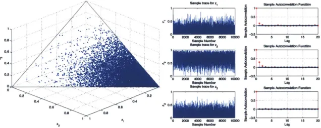
4-1 Case 1: Scatter plot of samples generated by the Gibbs sampling algo-rithm, along with the sample trace and autocorrelation plots ... 59
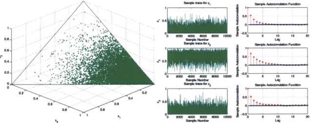
4-2 Case 2: Scatter plot of samples generated by the Gibbs sampling algo-rithm, along with the sample trace and autocorrelation plots . . . . . 59
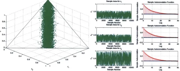
4-3 Case 3: Scatter plot of samples generated by the Gibbs sampling algo-rithm, along with the sample trace and autocorrelation plots . . . . . 60
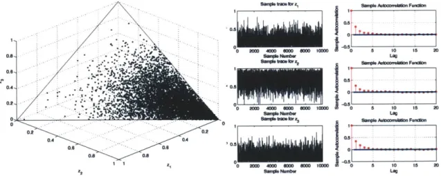
4-4 Case 1: Scatter plot of samples generated by the hit-and-run sampling
algorithm, along with the sample trace and autocorrelation plots . . . 61
4-5 Case 2: Scatter plot of samples generated by the hit-and-run sampling
algorithm, along with the sample trace and autocorrelation plots . . . 61
4-6 Case 3: Scatter plot of samples generated by the hit-and-run sampling
4-7 Case 1: Scatter plot of samples generated by the directional indepen-dence sampler, along with the sample trace and autocorrelation plots 63
4-8 Case 2: Scatter plot of samples generated by the directional indepen-dence sampler, along with the sample trace and autocorrelation plots 63
4-9 Case 3: Scatter plot of samples generated by the directional indepen-dence sampler, along with the sample trace and autocorrelation plots 64 4-10 Sample trace and autocorrelations along selected coordinates in the
Bayesian feed reconstruction example . . . . 66
4-11 Marginal densities of samples generated from Bayesian posterior dis-tribution for 2 different families of pseudo-compounds . . . . 67
4-12 Marginal densities of concentrations of pseudo-compounds in a partic-ular family for varying bulk concentrations . . . . 68
4-13 Comparing marginal densities of concentrations of pseudo-compounds in a particular family for varying degrees-of-belief in the bulk and lab-oratory measurements respectively . . . . 68 C-1 Plots observed samples for different values of
IIp,
with the populationList of Tables
4.1 Comparing the mean of the truncated normal distribution calculated using 2-D quadrature and the sample mean for the Gibbs sampler . . 60
4.2 Comparing the mean of the truncated normal distribution calculated using 2-D quadrature and the sample mean for the hit-and-run sampler 62 4.3 Comparing the mean of the truncated normal distribution calculated
using 2-D quadrature and the sample mean for the directional inde-pendence sampler . . . . 64
Chapter 1
Introduction
1.1
Feed reconstruction in chemical processes
In chemical plants and oil refineries, the typical process stream contains a mixture of a large number of molecular species. In oil refineries for example, it is not uncommon to observe streams with several thousand hydrocarbon species [19]. When these streams are used as a feed to reactors or unit operations in the plant, the detailed composition of the stream becomes important. Accurate knowledge of the stream composition in terms of the molecular constituents allows us to build good operating models (such as kinetic models), which in turn can be used control the reactor conditions, prod-uct yield and quality. Recent advances in analytical chemistry techniques (such as conventional gas chromatography (1D-GC) and comprehensive two-dimensional gas chromatography (GC x GC) [35]) allow us to to obtain detailed molecular composi-tions of various streams. However, these techniques are expensive, time consuming and rarely done in-plant. This means that it is not possible to analytically obtain the detailed composition of various streams in the plant on a regular basis. However, the dynamic nature of the modern refinery or chemical plant results in a changing stream composition on a daily, if not hourly, basis. To overcome this difficulty, it is common practice to resort to feed reconstruction techniques.
Feed reconstruction or composition modeling techniques are a class of algorithms that are used to estimate the detailed composition of a mixture starting from a limited
number of bulk property measurements (such as average molar mass, distillation data, specific density, atomic concentrations, etc.) [34]. In the absence of detailed experimental measurements, feed reconstruction algorithms provide a rapid way to obtain detailed composition data. These techniques have become increasingly popular with the rise of cheap computational power and the high cost of analytical techniques. To handle the sheer number of molecular components that are present in a typical feed, it is common practice to represent groups of molecules with a single represen-tative molecule called a pseudo-compound [19]. This procedure is also employed in analyzing the kinetics of complex mixtures of molecules, and is sometimes referred to as a lumping approach [22]. The pseudo-compound framework allows us to represent the stream with a significantly smaller set of species. However, it is still diffucult to experimentally ascertain the exact concentrations of these pseudo-compounds. We shall first elaborate on the pseudo- compound/lumping framework that we utilize here before we describe the general feed reconstruction process.
1.2
Pseudo-compound framework
The pseudo-compounds that are chosen to represent a particular feedstock must be sufficiently representative of the underlying actual molecular species to minimize any resulting lumping errors. In an oil refining context, the large number of hydrocarbons that that constitute any typical feed stream allow for a variety of pseudo-compound representations.
One popular choice of pseudo-compounds [19, 29, 35, 46] is based on identifying chemical families, which may be based on certain parameters, such as structural or reactive attributes. Once the chemical families are identified, the pseudo-compounds are then generated by choosing different carbon number homologues corresponding to each chemical family. For instance, if we identify the Thiophene family (molecules that contain at least one thiophene ring) as one possible constituent of our feedstock, then we may choose C1-Thiophene, C3-Thiophene and C7-Thiophene as pseudo-compounds to represent all members of the Thiophene family in the feedstock. The
chemical families that are identified often depend on the feedstock in question. Ana-lytical techniques can be used to understand the molecular composition of the feed-stock and reveal the types of chemical families that are required to model it. In Gas Oil feeds, for example, experimental analyses have been used to define 28 different chemical families that can be processed in a refinery [19], while a larger number of such families have been used to model vacuum gas oil cuts [46].
The carbon numbers corresponding to homologues of the chemical families are chosen based on the boiling range of the feedstock. Gas oil, which has a low boiling range, is typically composed of low carbon number molecules, while high boiling feeds such as vacuum gas oil require a higher carbon number range to model accurately.
This approach to feed modeling, which assumes that the given mixture of com-pounds can be described by a fixed library of pseudo-comcom-pounds , is said to be a deterministic representation of the feed. Stochastic representations, on the other hand, do not rely on a fixed library of pseudo-compounds. Instead, they rely on a distribution of molecular attributes and sample from this distribution to generate a realization of pseudo-compounds [29, 46]. However, stochastic methods are usu-ally difficult to implement because they are computationusu-ally intensive and rely on distribution information that is usually hard to obtain [50].
Ultimately, the choice of pseudo-compounds depends on the purpose and the de-sired accuracy of the modeling exercise. For low-fidelity models, it may be sufficient to pick a few chemical families and carbon number homologues. State of the art modeling [35, 34, 50, 27] techniques rely on generating a large number of chemical families by varying structural attributes and then using finely discretized carbon num-ber ranges. The modeler has to choose the pseudo-compounds appropriately, so as to reduce error in the estimation of any variables of interest.
1.3
Current approaches to feed reconstruction
Liguras and Allen [23] proposed one of the first feed reconstruction algorithms, which was based on minimizing a weighted objective function based on bulk measurements
collected using NMR spectroscopy. Their method was innovative, but it required a large number of property measurements to be effective. Since then, several different feed reconstruction techniques have been proposed.
Typical modern modeling techniques involve minimizing a specific function of de-viation of the observed bulk measurements from the calculated bulk measurements by varying the concentrations of the pseudo-compounds that are assumed to constitute the feed. Androulakis et al. [4] used a constrained weighted least squares approach to modeling the composition of diesel fuel. Van Geem et al. [45] proposed a feed reconstruction scheme that characterizes a given feedstock by maximizing a criterion similar to Shannon's entropy. Quanne and Jaffe propose a similar method, where the pseudo-compounds are replaced by vectors called Structured Oriented Lumping
(SOL) vectors. These methods assume that the feedstock being modeled can be
completely described by the fixed library of pseudo-compounds.
Alternative approaches to feed reconstruction have focused on coupling the mini-mization step with stochastic representation of the feed [29]. The pseudo-compounds are first generated using a Monte Carlo routine, and then their concentrations are calculated so that the computed bulk properties match the experimental measure-ments. Trauth et al. [44] used this method to model the composition of petroleum resid, while Verstraete et al. [46] adopted a similar idea to model vacuum gas oils. To reduce the computational burden associated with stochastic models, Campbell et al.
[9] used a Monte Carlo generation method coupled with a quadrature technique to
work with a reduced basis of pseudo-compounds. Pyl et al. [34] proposed a stochastic composition modeling technique that uses constrained homologous series and empir-ically verified structural distributions to greatly reduce the number of unknowns in the optimization step.
1.3.1
Drawbacks of current feed reconstruction schemes
While feed reconstruction schemes have been around for quite some time, they all suffer from similar drawbacks. The deterministic approaches to feed reconstruction sometimes require bulk properties that are hard to obtain, while the stochastic
ap-proaches rely on attribute distribution information that is mostly fixed on an ad-hoc or empirical basis.
In typical composition modeling techniques, it is difficult to add any new measure-ment information in a systematic manner. For example, if a modeler wishes to add a new type of bulk measurement to increase the accuracy of the predicted composition, it is not immediately obvious how one may modify the algorithm to incorporate this new piece of information. In particular, if we have any past detailed measurements that could improve current concentration estimates, we cannot take advantage of this information without significantly modifying the algorithm.
Furthermore, traditional composition modeling techniques do not incorporate a systematic idea of uncertainty in the reconstruction process. Understanding uncer-tainty in the composition of any feed stream in a chemical plant/refinery is very important. The uncertainty in the concentration of any pseudo-compounds of inter-est allows us to understand the impact of variation of bulk properties on the feed composition. Furthermore, the output of the feed reconstruction process might be used to model downstream unit operations like chemical reactors. In that case, hav-ing a handle on the input uncertainty to a unit operation gives us an idea of the resulting output uncertainty of the process. This becomes particularly important in applications such as oil refining, where the final product is expected to conform to certain quality standards. Having a low output uncertainty ensures that the quality of the product remains consistent across time.
Finally, from an experimental design point of view, an accurate quantification of uncertainty in the feed reconstruction process would allow us to analyze if we can reduce the uncertainty in any particular quantities of interest by incorporating addi-tional experimental measurements. For example, environmental regulations require a strict control on the level of sulphur in diesel produced in oil refineries. Therefore, it is important to estimate the composition of sulphur-containing psuedo-compounds with a high degree of confidence. However, it may only be possible to obtain a small number of bulk measurements. If we can quantify the uncertainty in the feed recon-struction, it is possible to implement an experimental design procedure to choose the
bulk measurements that yield the lowest level of uncertainty (or inversely, the high-est degree of confidence) in the concentrations of interhigh-est. The drawbacks that we have outlined in this section motivate the construction of a new feed reconstruction approach, by adopting a Bayesian approach to the problem.
1.4
Bayesian inference
Parametric inference is the branch of statistical inference that is concerned with iden-tifying parameters of a model given noisy data that is assumed to be generated from the same model. Traditional parameter inference frameworks (sometimes referred to as frequentist inference) assume that the parameters in a model are constant and any deviation in measurement from the model prediction is attributed to noise [48]. Typical frequentist inference techniques focus on finding a best estimate for each pa-rameter (also called a point estimate), along with an associated confidence interval.
The Bayesian approach to statistics is motivated by the simple idea that a prob-ability value assigned to an event represents a degree of belief, rather than a limiting frequency of the event. We can extend this notion of "probability as a degree-of-belief' to inference using Bayesian statistics. Contrary to frequentist inference, Bayesian in-ference assumes that the underlying model parameters are random variables. Bayesian parametric inference computes a probability distribution for each unknown param-eter from the data. Subsequent point estimates and confidence intervals are then calculated from the probability distributions.
Since the Bayesian inference procedure assigns probability distributions to each parameter, we need to choose a way to update the probability distributions with noisy data from the model. The most popular updating rule is the Bayes rule [41], which we shall describe below.
Let us denote the set of parameters as 0. First, we choose a probability distribution
p(9), called a prior, that reflects our beliefs about the parameters before observing
any data (denoted by D). Then, we choose a function C called a likelihood, which gives the probability of observing V, given 0. Then, by Bayes rule,
p(6|D) oc L(D|O)p(9) (1.1)
The posterior, p(ID), contains our updated belief on the value of 0 given D. Sometimes, the proportionality in (1.1) is replaced by an equality.The proportionality constant, denoted as, p(D) is termed as the evidence. It can be evaluated as
p(D) jL(D|9)p(9)d9
The Bayes rule provides a systematic way to update our beliefs regarding the values of the parameters of a model upon observing data that is generated from the model. The choice of the prior (p(9)) and the likelihood (L(D|j)) are very important, since they directly determine the accuracy of the estimated parameters.
1.5
Research objectives
The objectives of this research are twofold:
* Address the drawbacks of existing feed reconstruction schemes by recasting the problem into a Bayesian framework
" Review and develop efficient computational techniques to explore and analyze
the Bayesian model
1.6
Thesis outline
In chapter 2, we outline a Bayesian solution to the feed reconstruction problem. In chapter 3, we review some computational techniques to analyze the result of the Bayesian model. In chapter 4, we test the computational algorithms on some sample problems, and then use the best algorithm to analyze a Bayesian model developed on a dataset from a real refinery. In chapter 5, we summarize our conclusions from this study and provide some future directions to extend this work.
Chapter 2
A Bayesian inference approach to
feed reconstruction
In this chapter, we shall describe a Bayesian approach to the feed reconstruction problem. While we shall apply this feed reconstruction approach specifically to model crude fractions in an oil refinery, the general framework can be extended to other chemical systems.
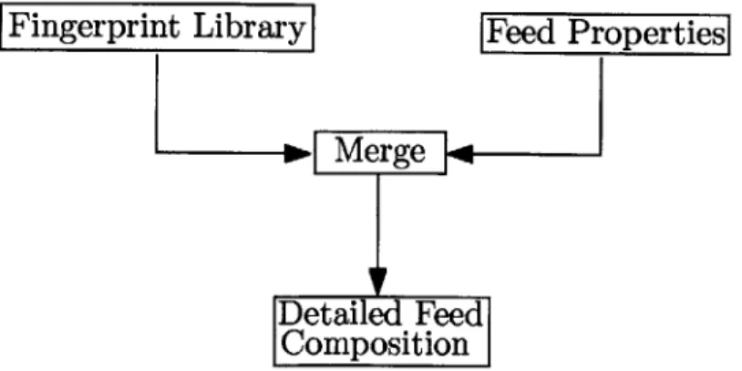
We are interested in developing a Bayesian model for the following framework: We have the detailed description for a particular type of feedstock in terms of the cho-sen pseudo-compounds from analytical chemistry techniques in a laboratory setting. These experiments are time-consuming and expensive, so we cannot repeat them on a daily basis in the chemical plant/refinery. Instead, we would like to predict the detailed composition from properties like distillation curves and bulk concentrations that can be easily measured in the plant. In this framework, a feed reconstruction model should combine the detailed information from the laboratory with the bulk information of the feedstock measured in the plant to infer the detailed composition of the feedstock in the refinery (in terms of weight percents/fractions). A schematic representation of this feed reconstruction procedure is presented in figure (2-1).
In the following sections, we shall first explain type of laboratory and plant infor-mation that we assume is available to the feed reconstruction process. Then, we shall outline the Bayesian inference procedure and elaborate on the details.
Fingerprint Library|
Figure 2-1: Feed reconstruction framework used to develop Bayesian model
2.1
Available data
2.1.1
Laboratory data
Detailed analytical techniques such as two-dimensional gas chromatography allow ex-perimentalists to identify the concentrations (in weight percent) of individual species with great precision. By applying these techniques on a sample feedstock (which is assumed to be representative of any typical feed that you might encounter in the re-finery), we can first identify a set of pseudo-compounds that can sufficiently describe the feed along with with their concentrations (in weight fractions) and molecular weights. The pseudo-compounds themselves are assumed belong to certain families, while individual pseudo-compounds within each family are differentiated by carbon number (as described in the previous chapter).
Since each pseudo-compound refers to a collection of molecules, it is not going to have a single boiling temperature. Instead, each pseudo-compound will boil over a temperature range. Along with their concentrations, we shall also assume that we can measure the initial and final boiling point of each pseudo- compound that is identified1.
'Since boiling information is a by-product of most detailed analytical techniques, this assumption is not unjustified
2.1.2
Plant data
The Plant Data refers to any bulk measurements of the feed that are collected in the refinery. While bulk measurements (or assays) could refer to a wide range of physical properties (such as atomic concentrations, refractive indices, specific gravities etc.), we assume that any assay that is collected in the refinery includes some distillation analysis (such as the ASTM D86 distillation [12]). At the simplest level, the resulting data can be understood as a set of boiling ranges and fraction of the crude that boils in those corresponding ranges.
These assumptions on data availability that we have made so far might seem restrictive at first glance. The subsequent analysis however, is general enough to deal with the absence of any type of information (albeit with slight modifications). We have chosen this particular structure in our data available since this refers to the most general type of data that is used as an input to a feed reconstruction procedure.
2.2
Bayesian formulation of feed reconstruction
The first step in constructing a Bayesian model for a given problem is to identify the parameters in the problem. Once we identify the parameters, we need to assign a prior distribution on the range of values that the parameters can take. Then, we need to define a likelihood function on the data that we observe. Finally, we need to use equation (1.1) to compute the posterior distribution on the parameters. In the following subsections, we shall construct a Bayesian model for the feed reconstruction problem using the same outline.
2.2.1
Target variable
Before we begin constructing probability distributions, we must first identify the parameters that we wish to infer in modeling the composition of any feedstock. First, we assume that the modeler has the pseudo-compounds of interest from the laboratory data and the boiling temperature ranges for the feedstock from the plant data. We
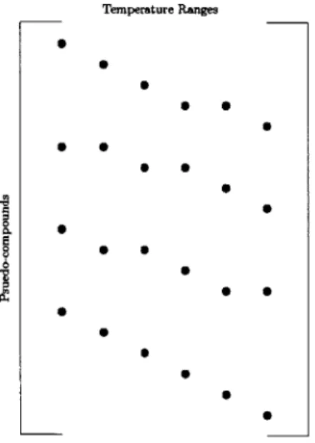
have to infer the concentrations of the various pseudo-compounds that are present in the feed in the plant. We shall infer the concentrations (in terms of weight fractions) as the entries of a matrix, where the rows correspond to various pseudo-compounds (that are identified in the laboratory), and the columns refer to the temperature ranges that the feed boils over (that is measured in the plant). The (ij)-th entry in this matrix denotes the the weight-fraction concentration of pseudo-compound i that boils in the j-th temperature interval. However, from the laboratory, we know that each pseudo-compound does not boil over every temperature range: For example, a pseudo-compound that boils in between 100 and 150* C, would not be expected to boil in a column corresponding to a temperature range of 200 to 4000 C. On the other hand, a pseudo-compound that boils over 150 and 350* C would be expected to have nonzero entries in the columns corresponding to 100 to 200* C and 200 to 4000 C. This idea enforces a great deal of sparsity in the structure of the matrix, which is sketched in figure (2).
Temperature Ranges
0
*
Figure 2-2: Grid of inference target weight fractions
It should be noted that there appears to be some additional structure in the ma-trix, since neighboring pseudo-compounds boil in consecutive temperature intervals. This is an artifact of the choice of our pseudo-compounds, since they are assumed to be members of the same family with differing carbon numbers. Our Bayesian
inference procedure will be focused only on the nonzero entries of the matrix. So while the procedure is explained in terms of this matrix, the final computations and mathematical operations are performed on a vector whose elements correspond to the nonzero entries of the matrix. We shall call this vector as our target variable of interest Y.2
2.2.2
Prior distribution
The prior distribution has to contain all the information about a feedstock before making any bulk measurements. In this case, the prior distribution has to encode the detailed laboratory data of a sample of crude that is similar to the feedstock in question. The choice of prior probability distribution has to ensure that the entries of Y are nonnegative and sum to one hundred (since they represent weight fractions). We model the distribution of entries in Y as a multivariate truncated normal distribution.
Truncated normal distribution
The truncated multivariate normal distribution is a probability distribution of a
n-dimensional multivariate random variable that is restricted to to a subset (S) of R". Mathematically, this distribution is calculated as
p(Y; y, E, S) oc exp
(-
p)T (y _ p 1 s(Y) (2.1)2
where yt and E are the mean and covariance parameters of the distribution re-spectively3, and 1s(Y) is an indicator function defined as
1 if Y E S 1s(Y)={
0 otherwise
2y can imagined as an "unrolling" of the matrix into a vector. For the purposes of understanding
the Bayesian model construction, Y can be imagined as either a matrix or a vector.
3
Note that these do not necessarily correspond to the mean and covariance of the truncated normal random variable. In this case, they are just parameters to the distribution.
Since p(Y) is a probability distribution, the normalizing constant (say, C) in equation (2.1) can be calculated as
C= - exp (y )TE-1(y Ii))dY
fs -2
In the feed reconstruction case, the subset S is defined as
S= {Y c Rj Yi = 1, Yi > 0, i =1...n}
i=1
The choice of the prior mean and prior covariance parameters for the distribution in equation (2.1) are detailed in the following sections.
Prior mean
The choice of the prior mean parameter is non-unique, and is a function of the type of information that is available. One particular choice (in this case, also the maximum likelihood choice) is the estimate of the entries of Y from the detailed analytical data. These estimates are not readily available, since there is is no accurate one-to-one correspondence between the the laboratory data and the entries of Y.
R1 R2 R3 R4
Si *
S2 * *
S3
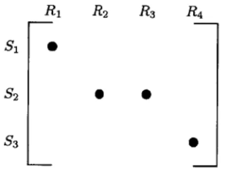
Figure 2-3: A schematic illustrating the "straddling" issue with assigning prior means, with a section for the matrix Y
For instance, in figure (2-3), the pseudo-compound S1 boils completely in the
temperature range R1. In this case, the prior mean of the nonzero entry corresponding
to pseudo-compound S1 would simply be concentration of S that is measured in the laboratory.On the other hand, the boiling range of a pseudo-compound could potentially straddle the temperature ranges corresponding to the columns of Y. The
pseudo-compound S2 has a boiling range that straddles temperature ranges R2 and
R3. This would imply that S2 has nonzero entries in the column corresponding to R4. However, there is no easy way to calculate the prior means corresponding to those nonzero entries.
One way to work around the mismatch in temperature ranges in the laboratory and the plant is to use an assumption on how the pseudo-compound boils in its temperature range. One valid assumption, for instance, is to assume that the pseudo-compound boils uniformly between its initial and final boiling point. In that case, the fraction of the pseudo-compound that boils in any arbitrary temperature range would be the ratio of the temperature range to the total boiling range. This assumption, although simple, is not really representative of how boiling occurs in practice. In this case, a more sophisticated assumption on the boiling profile of a pseudo-compound can improve the accuracy of the estimate of the prior mean.
Pyl et al. [34] observe that there is a correlation between the carbon number of
a hydrocarbon within a homologous series and its boiling point. In this particular feed reconstruction case, this idea would imply that there is a correlation between the boiling range and the carbon number of each pseudo-compound within a partic-ular family (which would be equivalent to a homologous series). Pyl et al. further suggest using an exponential or chi-squared distribution to model the relationship. Whitson et al. [49] suggest fitting a curve which takes the same functional form as a gamma distribution to petroleum fractions. While there are many choices to model the boiling profile of a feedstock , the gamma distribution is flexible and well-suited to the Bayesian reconstruction scheme. The details of the gamma distribution model are discussed below.
Mathematically, the gamma distribution is a function that models the probabil-ity distribution of a gamma random variable. The expression for the probabilprobabil-ity distribution is given by
oa t- t0) -1e48(t-to) ),if t > to
p(T = t; a,
#,
to) - r(t - (2.2)where a and
#
are 2 positive parameters of the gamma distribution, called shape and scale respectively. The parameter to is a shift term, which represents the lowest possible value of T that has a nonzero density value.This gamma distribution for the reconstruction case would be a function of the boiling point (T), and the area under the curve between any two boiling points would correspond to the weight fraction of the substance that boils in that temperature range. Furthermore, since equation (2.2) is a probability distribution,
p(t; a,
#)dt
= 1Using Pyl et al. 's suggestion, this gamma distribution is used to model the boiling profile within each family. If the shape (ak), scale (ak) and shift term (tk) are available for each family, it is possible to compute the weight fraction of any pseudo-compound that boils in a particular temperature range (as a fraction of the total family) using a simple procedure.
Suppose that pseudo-compound i (which belongs to a family k) boils in a temper-ature range [Li, U]. The fraction of pseudo-compound i that boils in any arbitrary temperature range [T1, T2] can be calculated as
0 , if T2 Li
fT2 p(t; ak/ ktk )dt ,if T1 < Li and T2 U,
f2 p(t; ak Ik,t )dt ,if T1 Li and T2 Uj (2.3)
ft
p(t; ak7 k,tk)dt , if T1 Li and T2 > U
0 , if T1 2 Ui
The resulting wi is a fraction of the concentration of the family k that boils as pseudo-compound i in the temperature range [T1, T2]. To convert this fraction into a
concentration of the pseudo-compound, an additional normalizing parameter for each family (say, ck) is required. Then, the final concentration of pseudo-compound i that boils in [T1, T2] is given by c k W
Given the parameters O@k - {k, /k, tk, ck}, this procedure provides a systematic way to populate the prior mean entries of Y. Now, all that remains is to to compute the parameters 4 k from the laboratory data.
Ideally, family k should not boil at any temperature below the lowest boiling point of all members (say, Lk). In other words,
p(t; ak, Ok,tk )dt = 0
This is consistent with a choice of tk = L .
Suppose that there are nk pseudo-compounds that belong to a particular family
k. The concentrations (ci, i = 1, ... , nk) of these pseudo-compounds are determined in the laboratory, along with their individual boiling ranges ([Li, Uj], i = 1, ... , nk).
First, the concentrations are normalized by their sum to result in weight fractions for each pseudo-compound wi = ci/
Ei
ci.Now, the values of ak,
#k
and ck have to be estimated from these quantities. First, Ck is chosen to be j ci. In other words, the total concentration of each family serves as an estimate of the normalization constant for each family. Then, the parameters ak and#k
have to be chosen such thatwi = P(t; ak 7k,tk )dt i = 1,... , nk (2.4)
/LUi0
LiSince p is a probability distribution, we can replace the integral in equation (2.4) with the cumulative distribution function F, which is defined as
F(T = t; ak, 3k, tk)a p(t;
j
a, tok tk)dt (2.5)When p is a gamma distribution, the expression for F can be written as
F(T = t;ak,Okjtk) -
-F(a)
where F is the gamma function, and -y is the lower incomplete gamma function [2]. Combining equations (2.4) and (2.5), we get,
wi = F(Ui;ak I k,tk) - F(Li;ak Ik,tk) i = 1,...,n (2.6)
Given the values of wi and [Li, U], i = 1,... ,nk, a statistical inference procedure
can estimate the values of ak and
#k.
A frequentist maximum likelihood approachcan be used to solve this problem to yield the "best" estimates for ak and
#k
for each family. This prior parameter estimation process is outlined in figure (2-4).Fingerprint I S
.1
I 0.I
0. Figure 2-4: Family Normalize EstimatePoint Data Point Data
I
A schematic illustrating the prior parameter estimation procedure
By this outlined procedure, it is possible to estimate a set of parameters 0'/
-{a
k, tk, t ck} (or in this case, hyperparameters to the prior mean) for each family from the detailed information from the laboratory. Once the parameters are es-timated, they can be used to compute the prior mean by the formula detailed in equation (2.3) and the following section.Prior covariance
Ideally, the prior covariance is a matrix whose (i, j)-th entry captures the how the concentrations of pseudo-compound i and
j
vary together. However, as a result of the large underconstrained nature of the feed reconstruction problem, it is often better to use some simplifying assumption to reduce the number of unknown covariance parameters. In this case, the prior covariance matrix E is assumed to be of the forma2
1m, where o > 0 is a variance parameter and Im is the m x m identity matrix. Now,
the only parameter that has to be tuned is o-.
The variance parameter indicates the degree-of-belief in the similarity of the feed that is analyzed in the laboratory and the feed that is being analyzed in the refinery.
If the 2 types of feed are believed to be similar (sourced from the same reservoir or
neighboring reservoirs, for example), then a lower value of the variance parameter can be used. If the two feeds are very different, then a higher value of variance would be appropriate.
2.2.3
Likelihood
If V denotes the vector of bulk measurements that are collected in the plant, then
the likelihood function L(DIY) is a function that quantifies how likely the observed plant data are, given realization of Y.
To construct this likelihood function, a measurement model is required. A mea-surement model is a function that calculates the bulk properties for a given realization of Y. If the vector of calculated bulk properties is denoted by Dck, the measure-ment model is a function
f,
such that Dac f(Y). For the sake of convenience,the Bayesian feed reconstruction model assumes that this function
f
is linear in Y. While this idea ensures that the expression for the posterior distribution can be de-rived analytically, this is not a necessary condition.While the linearity assumption might seem unjustified, the choice of the structure of Y makes it convenient to reconstruct several types of bulk measurements typically encountered in a refinery in a linear fashion. In the pseudo-compound and
tempera-ture matrix (which was described in the previous subsection), the columns correspond to the distillation temperature ranges. So, the weight fraction of the feed that is dis-tilled in each temperature range can be recovered as a simple column sum, which is a linear operation on Y. Bulk concentrations of atomic species, such as sulphur, can be calculated as
Scalc =i ) Yi (2.7)
where MWs is the molecular weight of sulphur, MWy, is the molecular weight of the pseudo-compound corresponding to Y. This is also a linear function of Y.
Since the calculated bulk properties can never match the actual observed bulk properties (D,), an error model on the observation is also required. For simplicity's
sake, a Gaussian measurement error is associated with each measurement. If the vector of observed bulk properties is denoted as DV,, then
(Dos) = (Dea1 c) + Ei, ei . A(O, of), i = 1, ... , nbulk (2.8)
where nekd is the number of bulk measurements. Here, ei is a Gaussian
measure-ment noise in the i-th bulk measuremeasure-ment with zero mean and variance o (which is usually available as instrument error). It is assumed that all the measurement errors are independent of each other.
With these assumptions, the likelihood function can be written as
£(DIY)
= exp (D' f (y)) TE 1(DP - (y)) (2.9)2
Em is a diagonal matrix where the (i, i)-th entry corresponds to the measurement
error in the i-th bulk measurement.
2.2.4 Posterior distribution
With the prior distribution and the likelihood, the posterior distribution can now be computed using equation (1.1) as
p(Y|D,) oc L(D,|Y)p(Y) (2.10)
If the prior is a truncated normal distribution, and the likelihood in equation (2.9) is used with a linear function f(Y) = GY (say), then a simple expression for
the posterior can be derived. From equation (2.10),
p(YID,) c L(D|Y)p(Y )
C exp (Dp - GY)TE -1(DP - GY) - p)TE-1(Y (Y)(Y
oc xp2 2 1s(Y
Using some algebra, this expression can be rearranged [40], to give
(Y - p TE) i t (Y - pt.0
p(YID,) oc exp (Y - 2 1s(Y) (2.11)
where
E. =(TF 1i G + E )- ; ypat = Epst G T E -1% 3
Zpost =(GT3l ±M Z) tM ~tT~ (2.12)
From equation (2.11), it is clear that the posterior is a truncated normal distri-bution as well, with the parameters stated in equation (2.12).
Equation (2.11) is a distribution over the nonzero entries of the matrix of pseudo-compounds and temperature ranges. The final distribution over the concentrations of the pseudo-compounds can be obtained with a simple row-wise sum. If Z represents a vector of concentrations of the pseudo-compounds, then Z can be computed using a linear of transformation of Y, say, HY. Then, the posterior distribution4 of Z is
p(ZID,) oc exp (Z - H1sost)T(HTEpostH)1(Y - Hip8t)) 1,(Z) (2.13)
4
Note that this expression is valid only when dim(Z) ; dim(Y), which is always true. Otherwise, the resulting covariance matrix will be improper
2.3
Advantages of the Bayesian approach
The Bayesian feed reconstruction procedure constructs a posterior distribution over the concentrations of each pseudo-compound by combining the laboratory informa-tion and plant data in a systematic manner. Unlike previous composiinforma-tion model-ing techniques, the explicit identification of the prior distribution and the likelihood makes it easy to add new sources of information while retaining intuitive knobs on the reliability of the new data, compared to existing information.
If a new kind of laboratory measurement is made, for instance, it can be
incor-porated into the reconstruction process by suitably modifying the prior distribution. On the other hand, if a new bulk measurement is made, it can be appended to the existing measurement vector D,, as long as it has an appropriate measurement model (preferably, linear) and an associated measurement error (of).
The notion of uncertainty is directly built into the Bayesian inference procedure. The concentrations Z are assumed to be realizations of a random variable with a multivariate probability distribution. Techniques to perform sensitivity analysis and experimental design on the reconstruction or any subsequent downstream process are readily available.
2.4
Exploring the posterior distribution
Inference procedures on random variables usually focus on expectations or integrals of the probability distribution function. For example, one quantity of interest to the modeler might be the average concentration, expressed as E(Z). To analyze the variation of the concentration of a pseudo-compound, the modeler might choose to analyze the percentiles of the probability distribution function (which is an integral of the density function).
The posterior probability distribution p(ZID,) is a high-dimensional distribution (since reconstruction procedures employ a high number of pseudo-compounds to im-prove modeling accuracy). While the expression for this distribution is simple, there
are no closed-form expressions to estimate the moments or expectations of this dis-tribution p(Z|D,).
To understand and utilize the resulting posterior distribution, there is a clear need to evaluate arbitrary expectations of Z. In the next section, we shall motivate the idea on how to evaluate these high-dimensional integrals.
Chapter 3
Computational aspects of feed
reconstruction
3.1
Introduction
In the previous section, a Bayesian formulation for the feed reconstruction problem was proposed and an expression for the posterior density function was derived. To analyze the posterior distribution, it often becomes necessary to evaluate integrals of the form
Ez[f(zi, .. . ,z.)] = ---. I
f(zi,
... ,z.)p(zi, .. ., z.)dS(zi,. . ., z.) (3.1) ScRnWhere Z is a random variable with a multivariate probability density function
p(zi,... , z,) that is truncated on a set S. In the feed reconstruction case, the
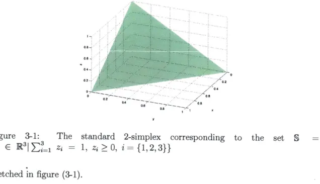
proba-bility density function would be the Gaussian density function with some mean and covariance parameters, and S would be the set
n
S= {z c R" n zi = 1, zi > 0, i = 1...n} (3.2)
/ 0 02
04 0.2J
Figure 3-1: The standard 2-simplex corresponding to the set S =
{z E R3|
1 =3 1, zi >O, i={1,2,3}}
sketched in figure (3-1).
In general, there are no analytical techniques to evaluate these integrals for cases where the density p(z) is the multivariate truncated normal distribution. These
distri-butions play an important role in a wide range of modeling applications even outside feed reconstruction [3, 28], so devising a good algorithm to evaluate these integrals is important. Numerical integration (or, quadrature) techniques are algorithms that are used to compute approximations definite integrals. If the integrals are univariate, there are several quadrature techniques that are readily available[32]. If the integrals are multivariate, numerical integration (or, cubature) using repeated application of
1D quadrature techniques does not scale well with the number of dimensions. For
high-dimensional numerical integration problems, Monte Carlo methods or sparse grid techniques are usually the methods of choice.
3.1.1
Monte Carlo methods
Monte Carlo (MC) methods are computationally intensive stochastic sampling tech-niques that can be used to numerically evaluate integrals. They rely on repeatedly sampling from random variables to carry out numerical computations. The idea was first proposed and developed by mathematicians and physicists at the Los Alamos labs during World War II. With the exponential increase in computing power, Monte
Carlo methods 1 are now very popular and widely used in different areas of compu-tational science.
One of the biggest advantages of MC methods lies in the scaling of the error in the numerical estimate Iet. If equation (3.1) is evaluated by repeatedly applying ID
quadrature techniques, the error bound |Iet - Il is O(N-r/d), where d is the number
of dimensions, and r is typically 2 or 4. As a result, typical quadrature methods become too computationally expensive outside low-dimensional (d < 7) problems.
However, the error bound in MC methods is O(N-1/2), independent of the number
of dimensions. This makes MC methods particularly attractive for high dimensional problems[1].
3.2
Numerical integration using Monte Carlo
sam-pling
The Monte Carlo integration algorithm numerically computes equation (3.1) by
gen-erating N random points zi, i = 1, ... , N, such that z~ p(z)), where p(z) is assumed
to be supported on S. Then, the value of the integral can be approximately computed as the arithmetic mean of the function evaluations at zi [24]. Mathematically,
Ez [f (zi, . . . , z.) ] ~zz IMC E~ - --. , z'), i =l1,2, -. -IN (3.3)
i=1
Note that this method can also be used to numerically integrate any function, if the probability density is chosen to be the uniform density function (assuming that S is compact) 2.
In the feed reconstruction problem, the probability distribution of interest p(Z) is
'It is worth mentioning that MC methods nowadays refer to a very broad class of algorithms. We are particularly interested in MC methods for numerical integration, so any mention of MC methods are in the context of numerical integration
2
While it might be tempting to evaluate Ez[f(zi,..., zn)] by numerically integrating g(Z)
f(Z).p(Z) using a uniform distribution, it should be noted that doing so would drastically reduce the accuracy of the Monte Carlo method[24]
3 a multivariate Gaussian distribution that is truncated on a simplex
Monte Carlo integration relies on the ability to generate (almost) independent samples from our truncated normal distribution p(z), to ensure the accuracy of the
Monte Carlo estimate[43]. While several sampling techniques exist in literature[24], the next section focuses on a particular class of methods called Markov Chain Monte
Carlo methods.
3.3
Markov chain Monte Carlo
Markov chain Monte Carlo (MCMC) methods are a class of algorithms that sample a probability distribution, p(z), by generating a Markov chain that has the same stationary distribution [18]. With the rise of computer processing power, there has been an explosion in the research and development of MCMC algorithms [8].
3.3.1
Literature Review
Geweke [17] first addressed the problem of sampling from a normal distribution sub-ject to linear constraints using an MCMC algorithm. However, the method was lim-ited and allowed only for a fixed number of inequality constraints. Rodriguez-Yam et
al. [38] extended Geweke's method to remove the restriction on the number of
con-straints, and introduced additional scaling in the problem to improve the sampling. Dobigeon et al. [13] explicitly address the problem of sampling from a multivariate Gaussian that is truncated on a simplex, by combining a Gibbs algorithm along with an accept-reject framework to sample from the 1-dimensional truncated Gaussian distribution [37].
Apart from the Gibbs family of algorithms, Smith et al. [6] proposed a particu-lar type of random walk samplers called Hit-and-Run samplers that can be used to sample from distributions restricted to convex domains. Recently, Pakman et al. [30]
3
For the sake of simplicity, this section will only discuss sampling from truncated normal
distri-butions. Sampling from arbitrary posterior distributions truncated on simplex-type constraints is
proposed a Hamiltonian Monte Carlo algorithm to sample from truncated Gaussian distributions.
3.3.2
Sampling problem
To analyze the results of the Bayesian model, we require samples from of the posterior distributions, which are multivariate normal distributions truncated on the standard simplex. However, for the sake of completeness, we shall analyze samplers that can generate samples from normal distributions that are truncated on convex polytopes4. Before we explore the different types of algorithms that can be used to sample from normal distributions truncated on convex polytopes, we can simplify the given sam-pling problem.
Consider sampling from the multivariate Gaussian distribution p(z) = N(p, E), such that the samples z obey
Amxnz = bmxi (34)
Ckxnz < d y1
where m and k are the number of equality and inequality constraints respectively. These feasibility constraints correspond to a convex polytope in R".
Note that the case of the truncated The Gaussian distribution can be conditioned such that the resulting function is a distribution only in the subspace defined by the equality constraints. This can be achieved by considering a new random variable
W = AZ, and deriving a joint distribution for the random variable pair V = (Z, W).
Once the joint is obtained, setting W = b, will result in a conditional distribution
p(ZIW = b).
Mathematically, the random variable W is Gaussian (since affine transformations of Gaussian random variables are Gaussian). This means that the joint distribution of Z and W is also Gaussian, with mean
i=
[[ p(Ap)T|T (3.5)and covariance
(3.6)
Then, the conditional distribution p(ZjW = b) = N(pc, Ec) [39], where
Ac = p' + E ETAT( AAT )-(b - Apt) (3.7)
and
EC = E- T AT(AEAT) -AE (3.8)
Now, any sample Z ~ (jp, Ec)", will obey the equality constraints in equation
(3.4).
Sampling from the n - m dimensional space spanned by the eigenvectors
corre-sponding to nonzero eigenvalues ensures that the resulting samples always obey the equality constraints. If we represent the eigenvalue decomposition of Ec as
Ec = QAQT (3.9)
If the zero eigenvalues and corresponding eigenvectors are deleted, then the trun-cated eigenvalue decomposition may be denoted as
EC =
UAUT
(3.10)This means that the problem can now be reparametrized in terms of an indepen-dent multivariate normal random variable W ~
N(O,
I), where I denotes an identity 5Ec is a rank-deficient covariance matrix, with rank = n - in-, where fii is the number ofinde-pendent equality constraints ( ; m) in equation (3.4)
rTAT
AEAT LAE
matrix, using the linear relation
Z= MW +pc (3.11)
where
M =
QA1/2
(3.12)Note that W is an (n - m)-dimensional random vector. The inequality constraints can be rewritten by substituting the expression in (3.11) in equation (3.4) as
Mw + Cyc < d (3.13)
where w denotes a sample of W. Now, the original problem reduces to one of sampling from a truncated (n - m)-dimensional independent multivariate Gaussian random variable, truncated to a convex polytope defined by equation (3.13).
In the following sections, 3 types of samplers Markov chain Monte Carlo samplers will be discussed.
3.3.3
Gibbs sampler
The Gibbs sampler [18] was introduced in MCMC literature by Gelfand and Smith [16] as a special case of the Metropolis-Hastings algorithm. The Gibbs algorithm for sampling from an arbitrary distribution p(w) truncated to a set S C R' is presented below:
Gibbs sampler
Step 1: Choose a starting point wo E S, and set i = 0
Step 2: Update each component of wz by sampling from the full conditional distributions along each coordinate, (i.e.)
Step 3: Set i= i + 1, and go to Step 2
In general, it is hard to obtain conditional distributions truncated to the feasi-ble set S. However, when the set S corresponds to a simplex (or more generally, a polytope), closed form expressions for the conditional distributions are easily avail-able [37].
A Gibbs type sampler can be implemented for this problem, since the conditional
distribution for each component is the standard normal distribution K(O, 1) truncated to a range. The lower and upper limits of this range can be computed using equation
(3.13).
Suppose that at iteration k, we wish to generate a sample of the i-th component
wk, say wk. The upper and lower limits of the conditional distribution range is given
by the minimum and the maximum of the vector wk , which is calculated as
S= d - Cyc - Mjii2j (3.14) where M,i denotes the matrix M with the i-th column removed, and Gej is the vector [wk . _1, k, -- ] The modified Gibbs algorithm can be
summa-rized as below:
Modified Gibbs sampler
Step 1: Choose a starting point w0 that satisfies equation (3.13), and set i = 0
Step 2: Update each component of W' by sampling from a truncated normal distribution along each coordinate, (i.e.)
w+1 ~
Nr(0,
1) , wj+1 G [a+1, b+1where a + and bj+1 are the minimum and maximum of w' 1, given by
equation (3.14)
To complete this procedure, we need to sample from a series of 1-dimensional truncated normal random variables. There are several algorithms [11, 37] available in literature to solve this problem, and any one can be suitably applied to sample from the conditional distribution at each step.
3.3.4
Hit-and-run sampler
d
Figure 3-2: Visual Representation of the Hit-and-Run algorithm. Image Courtesy: [20]
The Hit-and-run sampler is an MCMC algorithm that was first proposed by Smith [42] as an alternative to techniques such as rejection sampling and transforma-tion methods for generating uniformly distributed points in a bounded region. The Hit-and-run algorithm generates a Markov chain of samples by by first generating a direction d, and then sampling from the restriction of the bounded region on to the line passing through the current state, along the direction d. This idea is visually represented in figure (3-2).
Belisle et al. [6] extended the original Hit-and-run sampler to generate samples from arbitrary multivariate distributions restricted to bounded regions. Chen et
al. [10] modified and generalized the algorithm to the form that is used in this study.
The general Hit-and-run algorithm for generating samples from a random variable W with probability distribution p(w) supported on S(c R") is presented below: