A Bayesian latent time-series model for switching temporal interaction analysis

A Bayesian Latent Time-Series Model

for Switching Temporal Interaction Analysis

by Zoran Dzunic

B.S., Electrical Engineering and Computer Science, University of Nis, 2005 S.M., Electrical Engineering and Computer Science, MIT, 2009

Submitted to the Department of Electrical Engineering and Computer Science in partial fulfillment of the requirements for the degree of

Doctor of Philosophy in

Electrical Engineering and Computer Science at the Massachusetts Institute of Technology

February 2016

@ 2016 Massachusetts Institute of Technology All Rights Reserved.

Signature of Author:

Certified by:

Accepted by:

MAS HUSETS INSTITUTE 0 TECHNOLOGY

APR 152016

LIBRARIES

Signature redacted

Department of Electrical Engineering and Computer Science

i -January 29, 2016

Signature redacted

John W. Fisher III Senior Research Scientist, Electrical Engineering and Computer Science Thesis Supervisor

Signature redacted

I

k.

L/ U

Leslie A. Kolodziejski Professor of Electrical Engineering and Computer Science Chair, Committee for Graduate Students

A Bayesian Latent Time-Series Model

for Switching Temporal Interaction Analysis

by Zoran Dzunic

Submitted to the Department of Electrical Engineering and Computer Science in partial fulfillment of the requirements for the degree of

Doctor of Philosophy

Abstract

We introduce a Bayesian discrete-time framework for switching-interaction analysis under uncertainty, in which latent interactions, switching pattern and signal states and dynamics are inferred from noisy and possibly missing observations of these signals. We propose reasoning over posterior distribution of these latent variables as a means of combating and characterizing uncertainty. This approach also allows for answering a variety of questions probabilistically, which is suitable for exploratory pattern discovery and post-analysis by human experts. This framework is based on a Bayesian learning of the structure of a switching dynamic Bayesian network (DBN) and utilizes a state-space approach to allow for noisy observations and missing data. It generalizes the autoregressive switching interaction model of Siracusa et al. [50], which does not allow observation noise, and the switching linear dynamic system model of Fox et al. [16], which does not infer interactions among signals.

We develop a Gibbs sampling inference procedure, which is particularly efficient in the case of linear Gaussian dynamics and observation models. We use a modular prior over structures and a bound on the number of parent sets per signal to reduce the number of structures to consider from super-exponential to polynomial. We provide a procedure for setting the parameters of the prior and initializing latent variables that leads to a successful application of the inference algorithm in practice, and leaves only few general parameters to be set by the user. A detailed analysis of the computational

and memory complexity of each step of the algorithm is also provided.

We demonstrate the utility of our framework on different types of data. Different benefits of the proposed approach are illustrated using synthetic data. Most real data do not contain annotation of interactions. To demonstrate the ability of the algorithm to infer interactions and the switching pattern from time-series data in a realistic setting, joystick data is created, which is a controlled, human-generated data that implies ground truth annotations by design. Climate data is a real data used to illustrate the variety of applications and types of analyses enabled by the developed methodology.

Finally, we apply the developed model to the problem of structural health moni-toring in civil engineering. Time-series data from accelerometers located at multiple positions on a building are obtained for two laboratory model structures and a real building. We analyze the results of interaction analysis and how the inferred dependen-3

4

cies among sensor signals relate to the physical structure and properties of the building, as well as the environment and excitation conditions. We develop time-series classifi-cation and single-class classificlassifi-cation extensions of the model and apply them to the problem of damage detection. We show that the method distinguishes time-series ob-tained under different conditions with high accuracy, in both supervised and single-class classification setups.

Thesis Supervisor: John W. Fisher III

Acknowledgments

I would like to thank my advisor, John Fisher, for providing me guidance and support at every step of this road. His ideas and enthusiasm have been instrumental not only for my work, but also for broadening my views and growing as a researcher. I enjoyed numerous conversations with him over the years and timely jokes that he would often insert. I would also like to thank Bill Freeman and Asu Ozdaglar, members of my thesis committee, for questioning my work and providing me with invaluable comments that vastly improved the text of this thesis.

This thesis would not have been possible without help from other researchers. I would like to personally thank Justin Chen and Professor Oral Buyukozturk from MIT Civil Engineering Department, as well as Hossein Mobahi from the SLI group, with whom I had a fruitful collaboration on the structural health monitoring project. I owe big thank to Michael Siracusa, whose work I continued. He was so kind to meet with me many times to discuss his work, his code, and possibilities for then future work, which tremendously helped me get started on my own project. I also greatly enjoyed mentoring Bonny Jain, who worked on an extension of my model. I learned a lot from that experience.

Other members of the SLI group have always been there to help me. and they be-came really good friends. In no particular order, I thank Dahua Lin, Giorgos Papachris-toudis, Randi Cabezas, Sue Zheng, Julian Straub, Christopher Dean, Oren Freifeld, Guy

Rosman, David Hayden, Vadim Smolyakov, and Aryan Khojandi.

My everyday life at MIT has been joy thanks to my officemates. I would like to thank Ramesh Sridharan, George Chen, Giorgos Papachristoudis, Adrian Dalca, Danielle Pace, Polina Binder, Guy Rosman and Danial Lashkari for always being ready to help, talk and have fun, and for being the best officemates I could have asked for.

Finally, I would like to thank all of my friends and family. I especially thank my parents for their endless support. Most of all, I thank my lovely wife Ivana and my lovely daughter Lenka for their love, support and patience and for giving me a reason to look towards the future.

Different aspects of this thesis were partially supported by the Office of Naval Re-search Multidisciplinary ReRe-search Initiative program award N000141110688, the Army Research Office Multidisciplinary Research Initiative program award

6

Contents

Abstract 3 Acknowledgments 5 List of Figures 11 1 Introduction 17 1.1 Bayesian Approach ... ... 18 1.2 Contributions . . . . 20 1.3 O utline . . . . 22 2 Background 25 2.1 Bayesian Approach . . . . 25 2.2 Conjugate Priors . . . . 26 2.2.1 Exponential Families . . . . 27

2.2.2 Multinomial (Categorical) Distribution . . . . 28

2.2.3 Dirichlet Prior . . . . 30

2.2.4 Normal Distribution . . . . 31

2.2.5 Inverse-Wishart Prior . . . . 32

2.2.6 Matrix-Normal Inverse-Wishart Prior . . . . 33

2.3 Graphical M odels . . . .. . . . . 34

2.3.1 Directed Graphical Models (Bayesian Networks) . . . . 35

2.3.2 Temporal Directed Graphical Models (Dynamic Bayesian Networks) 36 2.4 Markov Chain Monte Carlo Sampling . . . . 37

2.4.1 Gibbs Sampling . . . . 38

2.5 Interaction graphs and DBN . . . . 39

2.6 Bayesian Learning of a Time-Homogenous Dependence Structure . . . . 39

2.6.1 Frequentist vs. Bayesian approach . . . . 41

Frequentist approach . . . . 41

Bayesian approach . . . . 41

2.6.2 Point estimation vs. full posterior distribution evaluation . . . . 43

8 CONTENTS

Point estim ation . . . . 43

Evaluatiing full posterior distribution . . . . 45

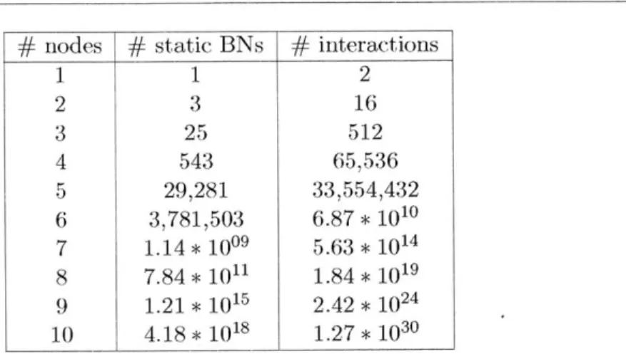
2.6.3 Complexity of Bayesian network structure inference . . . . 48

2.6.4 Prior for efficient structure inference . . . . 51

2.6.5 Related W ork . . . . 53

2.7 Bayesian Learning of Switching Dependence Structure . . . . 55

2.7.1 Batch sampling of the switching state sequence (step 1) . . . . . 57

3 SSIM: State-Space Switching Interaction Models 63 3.1 Related W ork . . . . 64

3.2 SSIM Framework . . . . 65

3.3 Linear Gaussian SSIM (LG-SSIM) . . . . 67

3.3.1 Latent autoregressive LG-SSIM . . . . 70

3.4 Gibbs Sampling Inference . . . . 72

3.4.1 Batch sampling of the state sequence (step 1) . . . . 73

3.4.2 Batch sampling of the state sequence in LG-SSIM model . . . . . 75

Algorithm with improved numerical stability . . . . 78

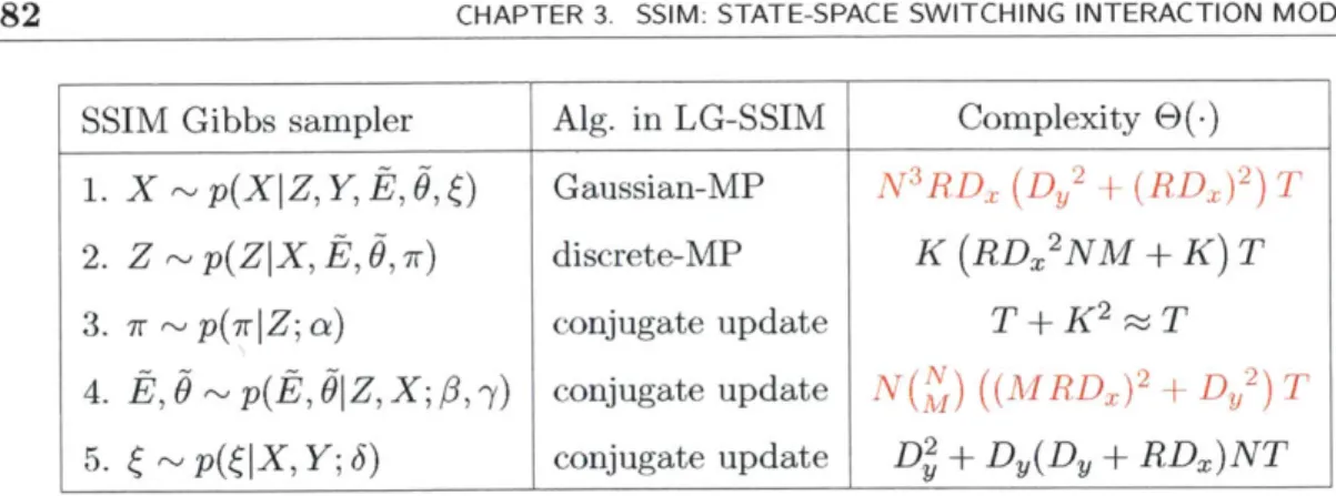
3.5 Algorithmic Complexity . . . . 79

3.5.1 Complexity of inference in LG-SSIM: step 1 . . . . 84

3.5.2 Complexity of inference in LG-SSIM: step 2 . . . . 85

3.5.3 Complexity of inference in LG-SSIM: step 3 . . . . 86

3.5.4 Complexity of inference in LG-SSIM: step 4 . . . . 86

3.5.5 Complexity of inference in LG-SSIM: step 5 . . . . 93

4 SSIM Experiments 95 4.1 Implementation and Practical Considerations . . . . 96

4.1.1 Setting Up The Prior . . . . 97

Prior on switching model . . . . 97

Prior on dependence models . . . . 98

Prior on the observation model . . . . 102

4.1.2 Setting up the Gibbs Sampler . . . . 103

Initializing Latent Variables . . . . 103

Gibbs Sampling Schedule . . . . 103

4.1.3 Evaluating the Posterior . . . . 104

4.2 Synthetic Data Experiments . . . . 106

4.2.1 Structure Inference vs. Pairwise Test . . . . 106

4.2.2 Observation Noise vs. No Observation Noise . . . . 108

4.3 Joystick Interaction Game . . . . 109

4.3.1 Comparison to other approaches . . . . 112

4.4 Climate Indices Interaction Analysis . . . . 113

5 Structural Health Monitoring with SSIM 119 5.1 Classification with SSIM . . . . 120

CONTENTS 9

5.2 Single-Class Classification wi 5.3 Experiments with Laborator, 5.3.1 Interaction Analysis

+h SSTIM

y Structures 5.3.2 Classification Results . . . .

Single column structure results 3-story 2-bay structure results 5.3.3 Single-Class Classification Results 5.4 Experiments with Green Building Data

5.4.1 Interaction Analysis . . . . 5.4.2 Single-Class Classification . . . . 6 Conclusion 6.1 Summary of Contributions . . . . Modeling . . . . Algorithms . . . . Experiments . . . . Structural Health Monitoring . . 6.2 Future Directions . . . . 6.2.1 Scalable inference . . . . 6.2.2 Nonparametric approaches . . . 6.2.3 Online learning . . . . 6.2.4 Multi-scale interaction analysis . 6.3 Final Thoughts . . . . A Computing messages mt(x) in LG-SSIM

Bibliography Data 124 126 127 129 130 132 134 137 138 139 145 145 145 145 146 146 147 147 147 148 148 149 151 153 CONTENTS ₉

CONTENTS 10

List of Figures

1.1 Dynamic Bayesian Network (DBN) representation of switching interac-tion among four signals. They initially evolve according to interacinterac-tion graph E1. At time point 4, the interaction pattern changes, and they

evolve according to interaction graph E2. Self-edges are assumed. . . . 19

2.1 (a) Undirected graphical model example: P(A, B, C, D, E) (x fi(A, B) f2(A, C) f3(B,D) f4(C,D) f5(B,D,E). (b) Directed graphical model example: P(A,B,C,D,E) = P(A) P(BIA) P(C) P(DIA,B,C) P(EIB,D). . . . . 35

2.2 Two examples of Bayesian networks. . . . . 36

2.3 Dynamic Bayesian Network (DBN) representation of a homogenous in-teraction among four signals with inin-teraction graph E. Self-edges are assum ed. . . . . 40

2.4 Frequentist homogenous temporal interaction model. . . . . 41

2.5 Bayesian homogenous temporal interaction model . . . . ... . . . 42

2.6 There are 16 possible interaction structures among 2 signals. . . . . 51

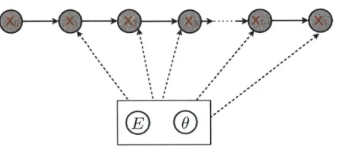
2.7 Switching temporal interaction model of Siracusa and Fisher [50]. . . . 56

3.1 State-space switching interaction model (SSIM). . . . . 66 4.1 The interaction structure in the two examples that demonstrate the

ne-cessity to consider parent sets rather than parent candidates individually. 107

LIST OF FIGURES

4.2 An example that demonstrates the advantage of modeling observation noise. (a) True interaction structure. (b) Posterior probability of edges obtained by inference in the STIM model (which does not model obser-vation noise). (b) Posterior probability of edges obtained by inference in the SSIM model (which models observation noise). The value at row

i and column

j

is the probability of edge i -+ j. Self-edges are blacked out, while the correct edges are marked with a white dot. Note that the STIM assigns probability 1 to a false edge 1 +- 3. Even though signal 1 depends only indirectly on signal 3 in the generative model, signal 3 helps explain signal 1 since the observations of signal 2 are noisy. On the other hand, if the SSIM is used for inference, the posterior probability of edge 1 +- 3 is significantly reduced. Note also that the probability of edge 3 <- 2 has increased, which means that the additional flexibility of the model may allow for different explanation of the data in the latent space. ... ... 108 4.3 (top) Three assignments of tasks. Individual tasks can be: F -- "follow",

M - "stay in the middle between", and "move arbitrarily" (otherwise). (bottom) Order and duration of assignments. . . . . 110 4.4 Interaction analysis on Joystick data when the maximum number of

parents is 3 (left) and 5 (right). Top row are the switching-state pair-wise probability matrices. Value at a position (ti, t2) is the probability that time points ti and t2 are assigned the same switching state, i.e.,

P(Ztl = Z 2). Note that in both cases there is an obvious switching

pattern that coincides with the setup of the experiment. A red block on the diagonal shows high probability that the corresponding time seg-ment is homogenous in terms of interaction (i.e., corresponds to a single switching state). A red off-diagonal block shows that time segments cor-responding to its projections onto

x

and y axes have the same interaction (are in the same switching state). Bottom row are edge posterior matri-ces at times 0.5, 1.25 and 2 min, which correspond to the three different assignments. The value at row i and column j is the probability of edge

i -+ j. Self-edges are blacked out, while the correct edges are marked with a white dot. Note that the SSIM assigns high probability to all correct edges and to a few spurious edges. Those errors commonly occur when two players have very similar behavior (e.g., players 2 and 3 both follow player 5 in the first assignment). Note also that there results are slightly worse when the maximum number of parents is 5, which is higher than needed. . . . . .111 12

4.5 Results on Joystick data when the number of switching state K is 2 (left) and 5 (right). Top row are switching similarity matrices. Bottom row are edge posteriors at times 0.5, 1.25 and 2 min. Note that even when

K is lower than the actual number of switching states (K = 2), the

switching similarity matrix indicates the presence of 3 states, and there are also three distinct interaction structures. The first result highlights the advantage of looking at the entire posterior distribution rather than at a MAP assignment. The second result is due to marginalization of the switching state sequence. Note also that when K is higher than the actual number of switching states (K = 5), the results are similar to those obtained with the correct number of states (Figure 4.4, left), which indicates that the additional states allowed are not assigned any new behavior that consistently appears in a large number of samples. . 112 4.6 Results on Joystick data when observation noise variance is 10-4 (left)

and when every 3 d value is observed (right). Top row are switching similarity matrices. Bottom row are edge posteriors at times 0.5, 1.25 and 2 min. Note that these results are qualitatively similar to those obtained from perfect data (Figure 4.4, left), even though relatively high noise is added to observation in one case and a large fraction (2/3) of observations are dropped in the second case. The uncertainty in the observation sequence is reflected in the posterior as a (slightly) higher uncertainty in the interaction structures and the switching pattern. . . 113 4.7 Results of structure inference on a segment of Joystick data that

corre-sponds to the second assignment (no switching), and to which high noise is added (variance of 10-3), obtained via: full inference in the SSIM model (left), full inference in the STIM model of Siracusa and Fisher [50] that does not account for the observation noise (middle), and MAP estimate in the SSIM model (right). Note that the SSIM assigns high probability to 3 out of 4 correct edges, while the STIM assigns high probability to only one of them. Also note that the SSIM assigns a re-duced probability (higher uncertainty) to the incorrect edge in the MAP structure (edge 4 -+ 5). . . . . .114

4.8 Analysis of the climate data using SSIM model. Top row is the switching-state pairwise probability matrix. Middle row is the Solar flux time series. Bottom row are the posterior probabilities of edges: Ninol2 -* GMT (blue), Ninol2 -+ Nino4 (red), Ninol2 -+ Nino34 (green). Note that the switching pattern exhibits a cyclic behavior that coincides with the cycles of Solar flux. The two states correspond to the low and high activity of Solar flux. . . . 115 4.9 Ninol2 (top) and ONI (bottom) time series. . . . 116 13

LIST OF FIGURES

4.10 Posterior edge probabilities on June 1963 (left) and August 1992 (right), which belong to the opposite phases of the cycle. Note that Nino indices (5-8) and ONI index (10) are the most influential overall, confirming that they are important predictors of climate. Interestingly, the only significant dependence of ONI index is on Southern Oscillation Index

(13). . . . . 117

5.1 SSIM model with multiple sequences. . . . . 121

5.2 SSIM model with multiple homogenous sequences. . . . . 121

5.3 Details of the laboratory setup . . . . 126

5.4 3D Visualization of node parent and child relationships with probability above 0.3. . . . . 128

5.5 Probability of parent nodes over many tests for intact and damaged cases. 129 5.6 Column structure data class-class log-likelihoods are shown as (a) matrix and (b) bar groups. Similarly, classification frequencies are shown as (c) matrix and (d) bar groups. . . . . 131

5.7 (a) Overall classification accuracy on column structure data as a function of training and test sequence lengths. (b) Classification frequencies (by test class) when training and test sequence lengths are 5K and 1K, respectively. . . . . 132

5.8 3 story 2 bay structure data class-class log-likelihoods are shown as (a) matrix and (b) bar groups. Similarly, classification frequencies are shown as (c) matrix and (d) bar groups. . . . . 133

5.9 (a) Overall classification accuracy on 3 story 2 bay structure data as a function of training and test sequence lengths. (b) Classification frequen-cies when training and test sequence lengths are 5K and 1K, respectively. 134 5.10 ROC curves for each damage scenario on 3-story 2-bay structure data. Points on the curves that correspond to the posterior probability of dam-age equal to 0.5 are marked with an 'x'. . . . . 135

5.11 Points of tradeoff between the rates of true positives and false positives when: (a) The threshold is set to L"' > Lt* ... > L , repsec-tively. (b) The threshold is set to ELju' + A-L "U for different values of A. ... .. ... 137

5.12 MIT Green Building . . . 138

5.13 3D Visualization of Green Building node parent and child relationships with incidence over 10% . . . . 140

5.14 Matrix visualization of node incidence for Green Building. The sensors are grouped into vertical sensors, EW sensors, and then NS sensors, as given in the axis labels. Concentration of high probability edges around the diagonal shows that many relationships are between the sensors in the same direction and close to each other. . . . . 141 14

LIST OF FIGURES

5.15 Matrix of the log-likelihood ratios, log Y 2(tt) between Green

Build-ing data sequences, normalized to be between 0 and 1. The value at row

i and column j corresponds to the ratio computed when sequence i is considered as a training sequence and sequence j as a test sequence. The correspondence between sequence indices and events is: 5/14/2012 Unknown Event (1), 6/22/2012 Ambient Event (2-3), Fireworks (4-6), Earthquake (7), 4/15/2013 Ambient Event (8-10), and Windy Day (11-16). Note that the events that are the most similar to each other are the events in ambient conditions, windy conditions, but also the first two sequences for the fireworks event, which were recorded before the fireworks actually started. On the other hand, the last sequence in the fireworks test case, the earthquake, and the 5/14/2012 event test cases all have significantly higher likelihood ratios with respect to the ambient cases. These results suggest that we can likely classify when the struc-ture has been excited in a significantly different way than typical ambient conditions. . . . . 143

Chapter 1

Introduction

E

XAMPLES of interaction can be found everywhere. One can talk about

an inter-action of people in a social network, at an event, or in a street, interinter-action of companies on a stock market, neurons in a brain, climate indices, and so on. Learning such interactions is important, as that can further our understanding of the processes among the involved entities, as well as lead to novel applications. However, while some interactions can be easily detected by our senses, a lot of them are still hard to identify by humans. Therefore, different sciences focus on inferring and analyzing interactions of different types and in different domains from data that can be related to interactions.

In this thesis, we consider the problem of inference over interactions from time-series data. The notion of interaction may be defined differently in different disciplines. For example, interaction between two objects often assumes a two-way influence between them. When more than two objects are involved, this would imply a two-way influence between any pair of objects, and inferring interactions would reduce to inferring groups (cliques) of objects that interact among each other. We are, however, interested in a more general case, in which an interaction is defined as any set of directed (one-way) influences among objects and the goal is to uncover such set of relationships, which we refer to as the structure of interaction. More formally, an interaction graph is defined as a directed graph G = (V, E), where V is the set of nodes that correspond to objects, and E is the set of edges that correspond to directed influences [50]. In other words, i -+ j E E if object i influences (has an effect on) object j, in which case we also say that object j depends on object i. We refer to the set of edges of the interaction

graph, E, as the interaction structure. In addition, we make the following assumptions: " Dependencies that constitute an interaction are temporal causal relationships [44], meaning that the behavior an object can only influence the future behavior of another object (or set of objects).

" Objects are represented as multivariate time-series (discrete-time multivariate signals). Therefore, we will often talk more abstractly about the interaction among time-series, or signals, where it will be assumed that these signals correspond to some objects or abstract entities, whose interaction is a subject of interest.1 1_{Note that we have not done analysis on the relationship between object representation (in terms}

CHAPTER 1. INTRODUCTION

Learning temporal interactions from time-series data is challenging for several rea-sons:

" The number of possible interactions among a set of signals is extremely large -super-exponential in the number of signals. Namely, if N is the number of signals, the number of possible interactions among them is equal to the number of different directed graphs, which is 2N2

" Interactions may change over time, and therefore the problem of learning interac-tion becomes the problem of learning different interacinterac-tions at different points in time and the pattern of switching between these interactions.

" Underlying time-series are often not observed directly, but rather through some noisy observation process. In additibn, data is sometimes missing due to an error or inability to collect observations at certain time points.

The first two problems have been addressed by the work of Siracusa and Fisher [49, 50], in which they develop a Bayesian switching temporal interaction model for in-ference over dynamically-varying temporal interaction structure from time-series data. However, their model assumes that time-series are observed directly and does not ad-dress the problem of noisy observations. On the other hand, switching state-space models have been used to learn switching joint dynamics of time-series from noisy data (e.g., [16,22]), but these models do not learn interactions among time-series. Our goal is to fill in the gap and develop a method that addresses all three challenges above in a single framework. To that end, we develop a state-space switching interaction model (SSIM) [13], which combines the two approaches, as well as an efficient Gibbs sampling algorithm for inference over latent time-series, interactions and the switching

pattern from noisy and (possibly) missing data in this model.

N 1.1 Bayesian Approach

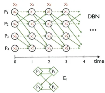
In addition to the assumptions above, we also assume that there exists a discrete-time stochastic process that generates future observations of discrete-time-series from their past observations, such that each time-series possibly depends only on a subset of other time-series. This naturally leads to a dynamic Bayesian network (DBN) repre-sentation of the joint time-series model, and the problem of inference over switching interaction is reduced to the problem of inference over a switching DBN structure (as in [50]), which is depicted in Figure 1.1. A fist-order model, in which the dependency is only on the values at the previous time point, is illustrated for simplicity. Moreover, we will first derive the SSIM model with a first-order dependency among time-series. However, we will later extend the model to allow higher-order dependencies.

of feature representation and sampling frequency) and the ability to infer temporal interactions using statistical methods.

Sec. 1.1 Bayesian Approach 19 x1.1 x1 x- x3 X4 X5 1

DBN

2 3 - -- -4 0 1 2 3 4 5 time 11 2

Ei

E2 4 4 3

Figure 1.1: Dynamic Bayesian Network (DBN) representation of switching interaction among four signals. They initially evolve according to interaction graph El. At time point 4, the interaction pattern changes, and they evolve according to interaction graph E2. Self-edges are assumed.

Inferring the structure of a (static or dynamic) Bayesian network presents a formidable

challenge owing to the super-exponential ninber of possible directed graphs. It, is known that, the exact inference over such structures is NP-hard in general [10]. A number of heuristic mnethods for finding a structure with the maximum a posteriori (MAP) probability have been developed [7, 11, 27]. However, MAP estimates of net-work structures are known to be brittle. With limited data available, there may exist a large number of structures that explain the data well. Point estimates of structure (e.g., MAP) are likely to yield incorrect interactions. The problem is exacerbated when the structure varies over time and time-series state is not observed directly, but rather by some noisy observation process. To alleviate this, sampling approaches have been typically used to approximate the posterior distribution over structures with a number of samples from that distribution [:9]. Due to the a typically highly-multimodal

pos-terior landscape, efforts have been made to develop robust sampling algorithms that do not get stuck in local optinma , 25, 39]. On the other hand., Siracusa and Fisher [5H] use a modular prior assumption, which effectively allows independent inference

over

parent sets of each time-series (that can be done in exponential time), and

ad-ditional

constraints

on possible parent sets (e.g., bounded in-degree), which result in a polynomial-time exact inference over a non-switching dynamic Bayesian structure, thus avoiding sampling

over

structure. These assmnptions have also been exploited in the context of static Bayesian

networks,

but since such

networks

imiust be acyclic. a topological order of nodes must either be known a priori [7, 11, 27] or sampled [19].

CHAPTER 1. INTRODUCTION

We adopt the approach of Siracusa and Fisher [50] and use a modular bounded-indegree prior on the interaction structure, which allows for efficient inference over structures. Also, as discussed above, computing a posterior distribution over structures quantifies the uncertainty in structure, and also allows for a robust estimate of structural events, which are often of primary interest. Examples of such events are: "Does object A depend on object B, given that it interacts with object C?" or "Which object is the most influential, i.e., has the most objects that depend on it?".

Note that the exact inference over structures is possible only if there is no switching and observations are assumed perfect. In case of switching and/or observation noise, exact joint inference over latent time-series, switching pattern and interaction struc-tures is intractable. Similarly as in [50], we use a Gibbs sampling approach to joint inference over these variables, in which an exact inference over interaction structures is performed when conditioned on other variables. However, unlike [50], where switching patterns obtained from different samples are aligned to produce a single most likely switching pattern, we reason over the distribution of switching patterns. This allows for computing statistics over switching patterns, such as the probability of two time points being in the same switching state. Consequently, there is no posterior distri-bution over structures defined for each switching state, since switching states are not aligned across samples. Instead, the switching pattern is marginalized out, and the posterior distribution over structure is computed for each time point separately, as it can indeed be different at each time point as a result of marginalization.

1.2 Contributions

The main contribution of the thesis is the introduction of a new model, which we refer to as the switching state-space interaction model (SSIM), and development of an efficient algorithm for Bayesian inference over switching interaction structure among time-series from noisy and possibly missing data [13], whereas the previous work assumes perfect observations [49, 50]. There are many examples where time-series measurements are noisy, such most data obtained through sensing, that motivate our method. For exam-ple, tracking objects in a video necessarily introduces observation noise, regardless of whether it is done by a human or an automatic tracker. Also, observations sometimes cannot be made due to occlusions, which results in missing data.

We introduce a linear-Gaussian variant of the SSIM, in which both time-series de-pendence and observation models are assumed linear and Gaussian. This specialization of the model is widely applicable and enables a particularly efficient inference procedure. We also introduce a latent-autoregressive linear-Gaussian SSIM, in which dependencies on an arbitrary number of previous time points are allowed. This extension is critical for many practical applications as first order models are often not sufficient to capture important dependencies. These two variants can be paralleled to analogous variants of the model of Siracusa and Fisher [49, 50], with the main distinction that their model does not incorporate an observation model.

Our approach extents the method of Siracusa and Fisher [49, 50] by introducing an observation model and assuming that the underlying time-series are in the latent space. While this extension is conceptually simple and intuitive, it poses several challenges that we address in this thesis. First, an additional step in an inference procedure for sam-pling latent time-series must be taken. Sequential samsam-pling of state sequences is know to converge slowly. Batch sampling can be done efficiently using an exact message-passing algorithm only for some choices of dependence and observation models. For example, this is the case when linear-Gaussian models are used. Otherwise, approxi-mate methods, such as particle filtering [2], must be employed. We take the advantage of the linear-Gaussian model and employ it in our work for efficient inference. How-ever, a standard message-passing algorithm for sampling latent time-series shows to be numerically unstable in cases when data is missing, in particular when there are several consecutive time-points for which data is missing. To alleviate that, we develop an alternative message-passing algorithm for this step that uses a different representation and computation of messages that is numerically stable. Second, the latent space in the SSIM model is very complex - latent interactions, switching pattern and time-series, as well as parameters of dependence and observation models need to be inferred from noisy and possibly missing observations. Jointly, these variables create a complex probability space. The posterior distribution over these variables is highly multimodal and there could be different suboptimal explanations of the data. For example, high variance of the dependence or the observation model can explain the data well, but that is not the explanation that is typically sought. Also, assigning time points to switching states is effectively a clustering problem, and spaces of clusterings typically have multiple local optima. To avoid undesired local optima and steer the inference into the regions of posterior distribution that are of interest, we develop specific methods for setting the prior and initializing latent variables. In addition, we often use multiple restarts to im-prove the coverage of the posterior distributions with samples. These methods lead to an algorithm that is mostly free of tuning, except for a few general model parameters. The new way of setting the prior also improves the previous method of Siracusa and Fisher [49, 50].

We demonstrate the utility of our approach on several datasets. Synthetic data is generated to emphasize the advantage over other methods. Specifically, we show that inference over the interaction structure as a graph is necessary, and that simply ana-lyzing pairwise dependencies separately (as in Granger causality tests [24]) may lead to a detection of spurious dependencies. We also show that our approach is advanta-geous over the previous method that does not account for observation noise [50] on an example in which the previous method assigns high probability to a spurious parent of a signal, because the correct parent does not predict well that signal alone due to the observation noise. When the observation noise is accounted for (our approach), the

probability of a spurious edge is significantly reduced.

Unfortunately, real datasets typically do not contain ground truth interactions. In-teractions are not know and are also difficult to annotate by humans due to their 21

CHAPTER 1. INTRODUCTION

complexity. This is, in the first place, a reason why learning interactions from data is an important task. However, it also renders testing inferred interactions difficult. To be able to test the results of interaction inference on non-synthetic data, we develop a new dataset, called joystick data, in which interactions and a switching pattern are known by design. Namely, five human players control points on a screen via joystick accord-ing to predefined tasks and a switchaccord-ing pattern between tasks. For example, a player can have an assignment to "follow" another player or to stay in the middle of the line between two other players. Therefore, interactions are implied by the tasks. We show that our method assigns high probability to the correct interactions and a switching pattern, and assigns significant probability to very few other (spurious) edges, even in the case of relatively high observation noise or if a significant portion (2/3) of data is missing. We also show that our method recovers the interaction structure better than the method of Siracusa and Fisher [50] in the case of high observation noise, as well as that our method assigns higher uncertainty to an incorrect edge in the MAP structure estimate, than to the correct ones. Lastly, we demonstrate the advantage of marginal-ization over switching pattern, which we employ,- over the previous method that only considers a point estimate of the switching pattern.

In addition, we apply our method to real datasets. While we cannot formally test the results of switching interaction analysis on them, we see that the results are co-herent with prior knowledge in the domain or general intuition. The climate indices dataset, Monthly atmospheric and ocean time series [40], consists of time-series of mea-surements of climate indices over several decades. Structural health monitoring (SHM) datasets are also used to perform interaction analysis. Buildings are instrumented with sensors (accelerometers) that measure vibrations at different locations. Two laboratory structures and one real building were used for experiments.

Finally, we develop extensions of the SSIM model for classification [14] and single-class single-classification of sequences of measurements, using an assumption that switching may only occur between sequences, and not within a sequence. These variants of the SSIM are applied to the problem of damage detection in civil buildings, which is one of the major problems in structural health monitoring. We demonstrate that our approach can detect damage or significant changes in the environment or excitation of a building with high accuracy, even in a single-class classification setup, in which only data from an intact structure is available for training (which is a typical case). The probability of a damage is in general higher for more severe damages. Also, the model can successfully differentiate different types of damages.

* 1.3 Outline

The organization of the thesis is as follows. The necessary background material is laid in Chapter 2. The SSIM, a framework for switching interaction analysis under uncertainty, which is based on a Bayesian state-space switching structure inference, is introduced in Chapter 3, along with the Gibbs sampling inference algorithm. The 22

Sec. 1.3. Outline 23

LG-SSIM, a specialization of the SSIM that uses linear-Gaussian dependence and ob-servation models, as well as the corresponding specialization of the inference procedure, are also presented in Chapter 3. Finally, the time and memory complexity analysis of the inference algorithm is also presented here. Practical considerations regarding setting the prior and initializing the latent variables are addressed in Chapter 4. Ex-periments on synthetic, semi-real and real data, which demonstrate the utility of the algorithm, are also presented in Chapter 4. Chapter 5 is devoted to the application of the developed framework to the problem of damage detection in civil engineering. Finally, conclusions and directions for future work are given in Chapter 6.

Chapter 2

Background

W

E take a Bayesian approach (2.1) to learning of the structure of

Dynamic Bayesian networks (2.3.2), which are probabilistic graphical models (2.3) suitable for mod-eling time-series data. The state-space modmod-eling paradigm is used to extend the pre-vious work ([49, 50], summarized in 2.7) to enable inference with imperfect (noisy and missing) data. In particular, a switching state-space approach is used to model the change in structure over time, in contrast to the switching auto-regressive approach used in [49, 50]. The inference is performed using a Gibbs sampling algorithm (2.4.1), which is a Markov chain Monte Carlo (MCMC) type of algorithm (2.4). A particular choice of probability distributions with conjugate priors (2.2) used for the dependence and observation models allows for efficient Gibbs sampling steps. Overview of the Bayesian learning of a homogenous (non-switching) dependence structure is presented in Section 2.6. Efficient inference over the space of structures, which is extremely large, is enabled by the use of a modular prior and a bound on the node in-degree (2.6.2).

N 2.1 Bayesian Approach

In contrast to the classical (or frequentist) approach, in which parameters of a statisti-cal model are assumed fixed, but unknown, in the Bayesian approach, parameters are assumed to be drawn from some distribution (called prior distribution or simply prior) and therefore treated as random variables. Let p(X 9) be a probabilistic model of a phenomenon captured by a collection of variables X, with parameters 9, and let p(G; 7) be the prior distribution of model parameters 9, parametrized by /, which are typi-cally called hyperparameters. The prior distribution is often assumed to be known, in which case hyperparameters are treated as constants and are either chosen in advance to reflect the prior belief in the parameters 9 (e.g., by a domain expert) or estimated from data (empirical Bayes, [8]). Alternatively, in a hierarchical Bayesian approach, hyperparameters are also treated as random variables and modeled via some distribu-tion, parametrized by a next level of hyperparameters, and so on, up to some level of hierarchy.

The central computation in Bayesian inference is computing the posterior distribu-tion of parameters 9 given data samples D = {XI, X2, .. ., XN}, namely, p(9

I

D; 7). If

the samples are independent, the data likelihood is p(1) 10) = p(X = kI JI 9). The

posterior distribution can be computed using the Bayes rule:

AOI AY) -p(6; -y) p(D 1)

_

p(; -Y) p(D )

(2.1)

A(D;Y) fop(6;y)p(D|1)dO

Note that the denominator p(D; -y), the marginal likelihood of data, does not depend on the parameters 0, which are "marginalized out". Therefore, the posterior distribution is proportional to the numerator:

A(

I

D; -Y) oc (0; -) p(D 10), (2.2) while the denominator is simply a normalization constant.

Evaluating the numerator above for a specific value of parameters is easy, as it is the product of the prior distribution and the data likelihood terms, which are specified by the model. However, computing the full posterior distribution p(0

I

D; -y), or even

evaluating it for a specific parameters value (which requires computing the marginal likelihood p(D; -y)), is in general difficult, as the posterior distribution and the marginal likelihood may not have closed-form analytical expressions. Nonetheless, when the prior distribution, p(0; 7), is chosen to be a so-called conjugate distribution to the likelihood distribution, p(X 6), the posterior distribution has the same form as the prior and can be computed efficiently.

M 2.2 Conjugate Priors

If the posterior distribution from Equation 2.1, p(O D; -/), is in the same family as the prior distribution, p(O; -y), then p(O; -y) is called a conjugate prior for the likelihood function, p(D 0). In that case, we say that the probability distribution p(D 16) has a conjugate prior. As a consequence, if the prior distribution has a parametric form (which we will assume in this thesis) and is a conjugate prior, then the posterior dis-tribution has the same parametric form and differs from the prior only in the value of hyperparameters, i.e., p(O D; -y) = p(0; -y') for some -y'. Note that -y' is a function of

prior hyperparameters -y and data D. Computing ^y' can be done analytically and is commonly referred to as "updating" the prior with the data or performing a "conjugate update".

Choosing a distribution that has a conjugate prior for a likelihood function and its conjugate prior for the prior is convenient as it results in an analytic form of the posterior, efficient computation of the posterior, and overall efficient inference in models that use such distributions. Otherwise, a computationally more challenging methods must be used, such as integration or sampling techniques. Also, interpreting conjugate updates is typically more intuitive than interpreting the results of numerical or sampling methods, as there is a meaning attached to the hyperparameters and how they are changed after a conjugate update.

Not all probability distributions have a conjugate prior. However, all distributions in the so-called exponential families, which includes a majority of well-known distri-butions, have a conjugate prior, and are therefore a convenient choice. We will proceed

Sec. 2.2. Conjugate Priors

by describing exponential families and the probability distributions that will be used in this thesis, all of which belong to the exponential family.

* 2.2.1 Exponential Families

An exponential family in the case of vector-valued variable X and parameters 6 (which is the case we will usually need in this thesis) is a set of probability distributions of the form:

p(XI 0) = h(X) exp {(O)T T(X) - A(G)} , (2.3)

where j7(6) is referred to as the natural parameter, T(X) as natural statistic or sufficient statistic, h(X) as the base distribution, and A(9) as the cumulant function or the log-partition function. Note that q(O) and T(X) are vectors, in general. An exponentially family is uniquely defined by the choice of 77(0), T(X) and

h(X), while A(9) is the logarithm of the normalization term implied by the previous

three functions:

A(O) = log

J

h(X) exp

{

7(0)TT(X)

}

dX, (2.4)

where the integral is replaced with a summation if X is a discrete variable. The nor-malization term, Z(O) - eA(O), is also called the partition function.

A linear exponential family is an exponential family whose natural parameter, ,q(O), is equal to the underlying parameter, 0:

p(X 0) = h(X) exp

{OTT(X)

- A(O)} . (2.5) Note that any exponential family can be converted into a linear exponential family by changing parametrization, i.e.,

p(XI0')

=h(X) exp {OITT(X) - A(G')}, where '= ,(0). However, finding the range of admissible values of 0' and the log-partition function

A(O') may pose a challenge.

A canonical exponential family is a linear exponential family whose natural statistics, T(X), is equal to the underlying variable, X:

p(XI 0) = h(X) exp

{OTX

- A(O)} . (2.6)

Exponential families have many useful properties. For example, the log-partition function play the role of a cumulant-generating function:

OA(X ) =~ E [Ti (X)| (2.7) a2 A(X) (27 a2 Aox) Cov [T(X)T₃(X)]. &0i&0j 27

28 CHAPTER 2. BACKGROUND Also, the natural statistic, T(X), is a sufficient statistic, which implies that all infer-ences about parameter 0 can be performed using T(X) - once T(X) is computed, the data X can be discarded. An important property of exponential families is that the dimensionality of the sufficient statistic, dim (T(X)), does not increase with the num-ber of data samples. To see that, let X1, X2, ... , XN be independent and identically

distributed (i.i.d.) random variables from a member of an exponential family defined by Equation 2.3. Then, the joint probability distribution of these variables is:

= N (N

p(X1, X2,... ,XN 10) =

(

h(Xi)) exp {7 (O)T

(

T(Xi) - NA(0) . (2.8)

i=1 =

Note that the sufficient statistic of all samples is simply the sum of sufficient statistics of each individual variable Xi.

The property of exponential families that will be the most important for us is that every exponential family has a conjugate prior. If the likelihood model of joint observations is given by Equation 2.8, then

p(O; r, no) oc exp {f Tr(0) - noA(0)} (2.9)

is a conjugate prior for that family, where r and no are hyperparameters. The posterior distribution over parameter 0 is

N )T

p( IX; r, no) oc exp

{(

+

>

T(Xi) r7(0) - (no + N) A(O) . (2.10) Clearly, the posterior distribution is in the same form as the prior, i.e.,

p(0IX; r, no) = p(; r', no') , (2.11)

where

N

-T = + ZT(Xi) _(2.12)

i=1

no' = no

+

N.

Therefore, performing a conjugate update is reduced to simply updating hyperparamters with the sufficient statistic and the sample count.

* 2.2.2. Multinomial (Categorical) Distribution

The multinomial distribution is a distribution over the possible ways of selecting N items from the set of K items, with repetition. Let i1, 72, - , IrK be the probabilities

of choosing items 1,2,... , K, respectively. Note that i_ 1 i =_ 1 must hold and N

Xi correspond to the number of times item i is selected. Then, the joint probability over X ₁, X2, . .., XK is

N! Mult(X1, X2, ... , Xk; 71 l2, .- - K) =

X

1

!XX1

7r 2 ... 7-K K, (2.13)

X1!X2! -.- XK!

where .X1, X2,. .. , XK are non-negative integers such that j=1 Xi = N. This

proba-bility can also be written using the gamma function as

r(EKXi + ) K

Mult(X1, X2, .X.. ,Xk X 2 1, .2, ,1K)

)

= (2.14)

Ui=1 r(Xi + 1) =1

which is a convenient form for a comparison to its conjugate prior - the Dirichlet distribution.

The mean and variance of a random variable Xi and covariance between Xi and Xj are given as:

E [Xi] Nxir

Var [Xi] Nrj(1 - 7rs) (2.15)

Cov [Xi, X]= -Nirxirj, i 3 j.

The categorical distribution can be thought of as the multinomial distribution with N = 1, i.e.,

K

Cat(Xi, X2,... , Xk; 7i1, 7r2, ... I IrK)

171-

(2.16)

i=1.

where exactly one of the variables X1, X2,..., XK is equal to 1, and the others are equal to 0. The categorical distribution is sometimes referred to as the discrete dis-tribution, since it is a distribution over a selection of one element from a discrete set of elements, where 7i is the probability of selecting element i. It is also commonly expressed using a single random variable X that takes a value from {1, 2,..., K}:

K

Cat(X; 71, r2,--- ,7rK = fri~, (2.17)

i=1

where [X = i] = 1 if X = i and [X = i] 0 otherwise. A connection to the represen-tation given in Equation 2.16 is established via equality Xi = [X = i]. Therefore, from

Equation 2.15, it follows that

E [[X -if]]= E[Xi] =7i

Var [[X =fl] = Var [Xi] =7ri(1 - 7ri) (2.18)

COV [[X = i] , [X =j]] = COV [Xi, Xj] = -7rigrj , i 54 j.

In machine learning, it is common to talk about a multinomial distribution when a categorical distribution is actually meant. Note also that the binomial distribution and the Bernoulli distribution are special cases of the multinomial and categorical distributions, respectively, in which the number of items, K, is equal to 2.

29 Sec. 2.2. Conjugate Priors

* 2.2.3 Dirichlet Prior

The Dirichlet distribution is a distribution over an open K-1-dimensional simplex in a K-dimensional space, which is defined as a set {(Xi, ... , xK) E K X >0 - , XK > 0,

Z:K

1 e= 1}. The probability density function of a Dirichlet distribution is given by

1

Dir(Xi, ... , XK; al,-, aK) = X1l- ... XKaK- 1, (2.19)

B(a1, .. .,aK)

where Ce, a2,..., aK > 0 and B(ai,..., aK) is the Beta function, which can be ex-pressed in terms of the gamma function as:

B(ai,..., CK) -

2=.l2

]p(EK_ (2.2)

The mean and variance of a random variable Xi and covariance between Xi and Xj are given as:

E [Xi] =

ceo

Var [Xi] = (ao-aj) (2.21)

a2(ao + 1) Cov [Xi, Xj] =-- ai e

ceo(Ceo + 1)

where ao = jai. Note that the mean of X does not depend on the absolute values

of parameters ai, but rather on their proportion. If all parameters a, are scaled by a same factor, the mean does not change. However, if that factor is greater than 1 (i.e., if parameters cei increase proportionally) and assuming that initially ai ;; 1, Vi, the

variance of each Xi decreases, meaning that the distribution on X₁, ... , XK becomes narrower around the mean.

Note that the support of the Dirichlet distribution is also the domain of possible distributions over a discrete set of K elements. Furthermore, the Dirichlet distribution is a conjugate prior to the multinomial (categorical) distribution. If the likelihood model is given by Equation 2.13 and the prior on parameters 1,.. .,rK as

Dir(,.rl,...,rKK q. al, C-O- -

aK

= 1 l.I- K aK1 (2.22)

j

1

F(ai)

and the observed valued are X1= c1,..., X = cK, then the posterior probability of

parameters is

'Dir(71, .. ., i=i i) 1, .e1_ .. -/ K l'-1

(2.23)~'K-Si=_1 r(a'i)

where a'1 = al + C, ... , a'K = aK + CK. Therefore, a Dirichlet conjugate update is

performed by simply updating each parameter ai with the number of samples from category i, ci. Parameters ai are also called pseudo counts as they are added to the observed counts. Having a prior parameter ai is equivalent to having a prior parameter ai - di and adding di pseudo observations from category i. Note from Equation 2.21

that the proportion of parameters aj determines the mean of probabilities ri, while their magnitude determines the variance of probabilities 7ri and thus reflects the strength of belief in the mean values. In general, the larger ai values are (the more pseudo-observations there are), the narrower the distribution on 7ri parameters is, meaning that the belief is stronger. Conversely, small values of ai parameters result in a prior with large variance, which is referred to as a weak (or broad) prior.

N

2.2.4 Normal Distribution

The (multivariate) normal distribution, also called the (multivariate) Gaussian

distribution, is a distribution over d-dimensional real vectors, X = [X1X2... Xd]T,

with a density function

exp(-!(X - p)TEl(X

-Ar(X; A,

E) =

27r d/2 1/2

,(2.24)

where p is a d-dimensional vector and E is a positive definite matrix of size d x d, which are also the mean and covariance matrix of X, respectively. I.e.,

E [X]

M

(2.25)

Cov [X]

=E,

which is a shorthand for the set of equalities

E [Xi] = pi

Var [Xi] =Ei (2.26)

Cov

[Xi, Xi = E .

A conjugate prior to the normal distribution with a known covariance matrix is also

a normal distribution. If the likelihood models is given as

p(X I

g;

E)

=

M(X;Ay, E)

(2.27)

and the prior on M as

p(p; tto, Eo) = A(,; go, Eo) , (2.28) and there are n independent samples of variable X, xl, . .. , x", then the posterior dis-tribution of the mean p is

(2.29) 31

Sec. 2.2. Conjugate Priors

CHAPTER 2. BACKGROUND

where

'=

(Eo~-

+ n E-1

(Eo~tpo

+ n

(2.30)

E/ = (Eo-1 + n E-')',

and t = 1 En₁ xi is the sample mean.

U

2.2.5 Inverse-Wishart Prior

The inverse-Wishart distribution is a distribution over positive-definite matrices of a fixed dimension, d x d, with a density function

IV(X; T, ,) - IXI-(+d+l)/2

exp-1

tr(VX_1)), (2.31)

2nd/2 'd(rs/2) 2

where dO is the multivariate gamma function [30], r, > d - 1 is a scalar parameter

called the degrees of freedom, and 4' is a d x d positive definite matrix parameter called the inverse scale matrix.

The mean and the mode of an inverse-Wishart distributed random matrix X are not equal:

E [X] = , > d+ 1

S,-d-1

_(2.32)

Mode [X] = _{r, + d + I}.

For larger values of , the variance of X is smaller, and therefore the distribution is narrower around the mode.

The inverse-Wishart distribution is a conjugate prior to the normal distribution with a known mean. If the likelihood models is given as

p(X

I

E; [) =

Af(X;

yu, E) (2.33) and the prior on E as

p(E; T, K) = IW(E ; I,

K),

(2.34)

and there are n independent samples of variable X, X1..., ,n, then the posterior dis-tribution of the covariance matrix E is

p(E

I21 J.

. . ,X"';

*, r)

=IW(E;

V, W'),

(2.35)

where

n

T = 4 + ](xi - i)(xi - )(236) i= 1

W' =, + n.

Note that setting a small value of , defines a weak (broad) prior on E, and that /- can also be thought of as a pseudo-count.