Augmenting Physics Simulators with Neural
Networks for Model Learning and Control
by
Anurag Ajay
B.S., University of California, Berkeley 2017
Submitted to the Department of Electrical Engineering and Computer
Science
in partial fulfillment of the requirements for the degree of
Master of Science in Computer Science and Engineering
at the
MASSACHUSETTS INSTITUTE OF TECHNOLOGY
June 2019@
Massachusetts Institute of Technology 2019.
Author ...
All rights reserved.
Signature redacted
Department of Electrical Engineering and Computer Science
Certified by..
Certified by.
Signature redacted
May 16, 2019
Leslie P. Kaelbling
Prreor,4 Ele Iita Engineering and Computer Science
3ignature redacted
Thesis Supervisor
Ci
Joshua B. Tenenbaum
Professor of Brain and Cognitive Science
Signature redacted
Thesis Supervisor
Accepted by
MASSACHUSETS INSTITUTE OF TECHNOLOGYJUN 13 2019
' U C Leslie A. KolodziejskiProfessor of Electrical Engineering and Computer Science
Chair, Department Committee on Graduate Students
....Augmenting Physics Simulators with Neural Networks for
Model Learning and Control
by
Anurag Ajay
Submitted to the Department of Electrical Engineering and Computer Science on May 16, 2019, in partial fulfillment of the
requirements for the degree of
Master of Science in Computer Science and Engineering
Abstract
Physics simulators play an important role in robot state estimation, planning and control; however, many real-world control problems involve complex contact dynamics that cannot be characterized analytically. Therefore, most physics simulators employ approximations that lead to a loss in precision. We propose a hybrid dynamics model, combining a deterministic physical simulator with a stochastic neural network for dynamics modeling as it provides us with expressiveness, efficiency, and generalizability simultaneously. To demonstrate this, we compare our hybrid model to both purely analytical models and purely learned models. We then show that our model is able to characterize the complex distribution of object trajectories and compare it with existing methods. We further build in object based representation into the neural network so that our hybrid model can generalize across number of objects. Finally, we use our hybrid model to complete complex control tasks in simulation and on a real robot and show that our model generalizes to novel environments with varying object shapes and materials.
Thesis Supervisor: Leslie P. Kaelbling
Title: Professor of Electrical Engineering and Computer Science
Thesis Supervisor: Joshua B. Tenenbaum Title: Professor of Brain and Cognitive Science
Acknowledgments
Contents
1 Introduction 15
1.1 Physics Engines as dynamics model . . . . 16
1.2 Residual learning with physics engine . . . . 17
1.3 Object-based residual models for control . . . . 18
2 Related Work 21 2.1 Models for Planar Pushing . . . . 21
2.2 Differentiable Physical Simulators . . . . 22
2.3 Learning Contact Dynamics . . . . 22
2.4 Uncertainty Modeling . . . . 24
2.5 Control with a Learned Simulator . . . . 24
2.6 Residual Policy Learning . . . . 25
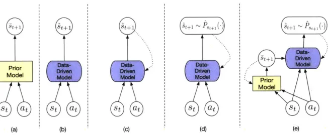
3 Formulation 27 3.1 Prior M odel . . . . 27
3.2 Data-Driven Model . . . . 28
3.3 Recurrent Data-Driven Model . . . . 29
3.4 Stochastic Recurrent Data-Driven Model . . . . 30
3.5 Stochastic Recurrent Data-Augmented Residual Model . . . . 31
4 Residual Learning with Stochastic Neural Networks 33 4.1 Variational Recurrent Neural Network . . . . 33
4.3 Decoupled Conditional VRNN . . . . 36
5 Residual Learning with Object-based Networks 39 5.1 Interaction Network . . . . 39
5.2 Simulator-Augmented Interaction Networks . . . . 40
5.3 Stochastic Interaction Network . . . . 42
5.4 Stochastic Simulator-Augmented Interaction Networks . . . . 45
6 Control with Object-based Neural Networks 49 6.1 Control Algorithm for SAIN . . . . 49
6.2 Control Algorithm for SSAIN . . . . 50
7 Experiments 51 7.1 Model Learning with Decoupled Conditional VRNN . . . . 51
7.1.1 Experiments with Bouncing Balls . . . . 51
7.1.2 Experiments on Planar Pushing . . . . 54
7.2 Model Learning with Object-Based Neural Networks . . . . 60
7.2.1 Experiments on Multi-Object Planar Pushing in Simulation 61 7.2.2 Experiments on Multi-Object Planar Pushing in Real World 65 7.3 Control with Object-Based Neural Networks . . . . 66
7.3.1 T ask . . . . 67
7.3.2 Search Algorithm . . . . 68
7.3.3 Control Results in Simulation . . . . 70
7.3.4 Control Results in Real World . . . . 72
8 Discussion and Conclusion 75
List of Figures
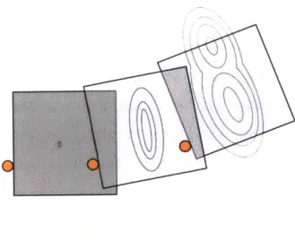
1-1 The motion of an object being pushed appears stochastic and possibly multi-modal due to imperfections in contact surfaces, non-uniform coef-ficient of friction, stick/slip transitions, and micro surface interactions. 17
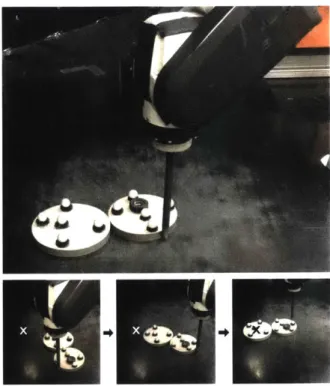
1-2 Top: the robot wants to push the second disk to a goal position by pushing on the first disk. Bottom: three snapshots within a successful push (target marked as X). The robot learns to first push the first disk to the right and then use it to push the second disk to the target position. 19
3-1 Model classes: (a) prior model; (b) data-driven model; (c) recurrent data-driven model; (d) stochastic recurrent data-driven model; and (e) stochastic recurrent data-augmented residual models. . . . . 28
4-1 Illustrations for VRNN: (a) computing conditional prior of zt using Eq 4.5; (b) generating xt using Eq 4.4; (c) updating hidden RNN state ht
using Eq 4.12; (d) inference of approximate posterior for zt using Eq 4.1. 34
4-2 Illustrations for conditional VRNN: (a) computing conditional prior of
zt using Eq 4.11; (b) generating xt using Eq 4.4; (c) updating hidden RNN state ht using Eq ??; (d) inference of approximate posterior for
zt using Eq 4.9. . . . . 35
4-3 Illustrations for decoupled conditional VRNN: (a) computing condi-tional prior of zt using Eq 4.18; (b) generating xt using Eq 4.16; (c) inference of approximate posterior for zt using Eq 4.14. . . . . 37
5-1 (a) Interaction network (IN) applied to object 1 in an environment with 3 objects using Eq 5.1 (b) Simulator Augmented Interaction network (SAIN) applied to object 1 in an environment with 3 objects using Eq 5.5. 41 5-2 Illustrations for SIN applied to object 1 in an environment with 3
objects: (a) computing conditional prior of zt+1 using Eq 5.20; (b)
generating ol+1 using Eq 5.12; (c) updating hidden RNN state h'+1
using Eq 5.22; (d) inference of approximate posterior for z' 1 using Eq
5.10. ... ... ... ... . . . . 42
5-3 Illustrations for SSAIN applied to object 1 in an environment with 3 objects: (a) computing conditional prior of zl+1 using Eq 5.20; (b)
generating o+1 using Eq 5.23; (c) updating hidden RNN state h'+1
using Eq 5.22; (d) inference of approximate posterior for z'+1 using Eq
5.10. ... ... ... ... 46
7-1 The two scenarios: ball bouncing and planar pushing. . . . . 52
7-2 Prediction errors vs. training data size. Our hybrid model not only performs better, but also requires much less data to achieve a given level of performance. In contrast, purely using purely data-driven models requires a larger training set and is not performing as well. . . . . 55
7-3 Our Hybrid model captures the distribution of possible push outcomes. Measured in Chamfer distance, our model achieves a lower error com-pared with GP-SUM [4]. . . . . 57
7-4 Our method generalizes well to different materials and to a new shape
(rect2 in the push dataset). The error bars show our hybrid model
achieves a consistently lower generalization error for both position and rotation prediction, compared with baseline methods. . . . . 58
7-5 SSAIN model captures the distribution of possible push outcomes . . 62
7-6 Qualitative results and success rates on control tasks in sim-ulation. The goal is to push the red disk so that the center of the blue disk reaches the target region (yellow). The transparent shapes are their initial positions, and the solid ones are their final positions after execution. The center of the blue disk after execution is marked as a white cross. (a) Control with SIN works well but makes mistakes occasionally (column 3). (b) Control with SSAIN achieves perfect performance in simulation. . . . . 67
7-7 Control with SSAIN and SAIN: Qualitative differences between control with a stochastic model (SSAIN) and control with a deterministic m odel (SA IN ) . . . . 68 7-8 Results on control tasks in the real world. The goal is to push
the red disk so that the center of the blue disk reaches the target region (yellow). The left two columns are examples of easy pushes, while the right four show hard pushes. Top: The model trained on simulated data only performs well for easy pushes, but sometimes fails on harder control tasks; Bottom: The model trained on simulated and real data improves the performance, working well for both easy and hard pushes. 69 7-9 Generalization to new scenarios. (a) SAIN trained generalizes to
control tasks on a new surface (plywood), with a success rate of 92%; (b): It also generalizes to tasks where the two disks have a different radius (red: small -+ large; blue: large -* small), with a success rate of
List of Tables
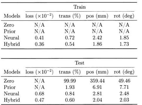
7.1 Our hybrid model achieves the best performance in both position and velocity estimation of the ball, compared with methods that rely on physics engines or neural nets alone . . . . 52 7.2 Our hybrid model achieves the best performance in both position and
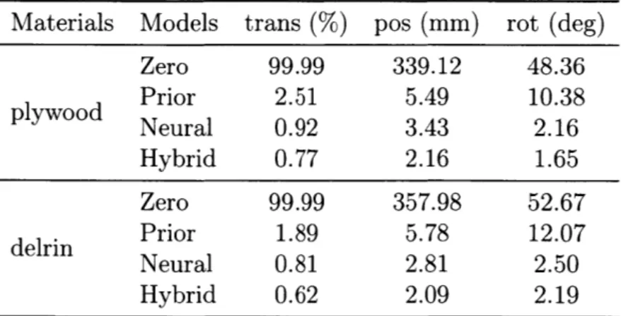
rotation estimation for recti, compared with methods that rely on physics engines or neural nets alone. Here we show results on both training and test sets, as well as the optimization losses. These numbers suggest that our Hybrid model is overfitting to the training set less than the pure Neural model. As we focus on long-term prediction, we include the Zero baseline to show the scale and the challenging nature of the problem . . . . 53 7.3 Our Hybrid model performs well consistently across object materials.
Here for the rectangle made of plywood and delrin, our model again outperforms all other baseline models. . . . . 54
7.4 Errors on dynamics prediction in direct-force simulation setup. SSAIN achieves the best performance in both position and rotation estimation, compared with methods that rely on physics engines or neural nets alone. The first two metrics are the average Euclidean distance between the predicted and the ground truth object reported as a percentage relative to the initial pose (trans) and as absolute values (pos) in millimeters. The third is the average error of object rotation (rot) in degree. . . . . 60
7.5 Generalization to 3 objects in direct-force simulation setup. SAIN achieves the best generalization in both position and rotation estim ation . . . . 60 7.6 Errors on dynamics prediction in robot control simulation
setup. SAIN achieves the best performance in both position and rotation estim ation . . . . 61
7.7 Errors on dynamics prediction in the real world. SAIN obtains
the best performance in both position and rotation estimation. Its performance gets further improved after fine-tuning on real data. . . . 65
Chapter 1
Introduction
A model of the world dynamics is important for planning and control in robotics. To plan for a task, a robot may use its dynamics model to simulate the effects of different actions on the environment and then select a sequence of them to reach a desired goal state. The utility of the resulting action sequence depends on the accuracy of the dynamics model's predictions, so a high-fidelity dynamics model is an important component in robot planning.
Given recent success of machine learning, especially deep learning, in fields like computer vision, natural language processing, reinforcement learning, etc. it is natural to think about learning a dynamics model using some parametric model, like neural networks. But, as has been frequently observed, neural networks require lots of data for training. To make the learning data efficient, we often introduce some inductive bias in the neural networks (or other learning models) in form of some architectural choices. One of the simplest forms of inductive bias is to make the neural network linear. Though this bias makes learning data efficient, the limited representational capacity of linear neural networks significantly diminishes overall performance.
In this thesis, we look at another inductive bias, in form of residual learning, to make learning data efficient. We assume that we have some prior model which performs the task partially with some errors but which is cheap to evaluate. In this work, since we want to learn a dynamics model, a prior model would take in the current state and action and return next state after some fixed time interval with some
error. On top of prior model, we have a residual model, which is learned, and which takes in the current state and action as well as the prediction by the prior model and learns the discrepancy between ground truth and the prediction by the prior model. The residual model could be some parametric model like a neural network. Again, since we want to learn a dynamics model, the residual model takes in the current state and action and the next state prediction from the prior model and outputs its own prediction of the next state. Overall, our proposed framework has two components: a prior model which is fixed and a residual model which is learned.
A question still remains: Where do we get our prior model? Generally, a prior model could be a software artifact such as a commercial game physics engine or a hand-designed analytical model which solves the task partially with some errors. In this work, our goal is to learn a dynamics model which can be used for control. Luckily, there already exists physics-based analytical models or software packages based on
approximate physics (called physics engines) which can approximately simulate future states given current state and action. In this work, we use a physics-based analytical model or physics engine as our prior model.
1.1
Physics Engines as dynamics model
Most physics engines used in robotics (such as ODE [40], Mujoco [42] and Bullet [121) rely on approximate and efficient dynamics models and do not reason about uncertainty explicitly. While they are an important tool, their practicality has been limited due to discrepancies between their predictions and real-world observations. A major source of mismatches is the contact models used in these simulators. Contact is a complex physical interaction with near impulsive forces over a small duration of time that involves local deformations and vibrations. Matters are complicated by the sensitivity of contact outcomes to initial conditions. These models are coarse approximations to contact, and recent studies ([29],
[451,
[16]) have shown the discrepancies between their predictions and real-world data. These mismatches make contact-rich tasks hard to solve using these physics engines.Figure 1-1: The motion of an object being pushed appears stochastic and possibly multi-modal due to imperfections in contact surfaces, non-uniform coefficient of friction, stick/slip transitions, and micro surface interactions.
One way to increase the robustness of controllers and policies resulting from physics engines is to add perturbations to parameters that are difficult to estimate accurately (e.g., frictional variation as a function of position [45]). This approach leads to an ensemble of simulated predictions that covers a range of possible outcomes. Using the ensemble allows to take more conservative actions and increases robustness, but does not address the limitation of using learned, approximate models [32, 61.
1.2
Residual learning with physics engine
To correct for model errors due to approximations, we learn a residual model between
real-world measurements and a physics engine's predictions. Combining the physics engine and residual model yields a data-augmented physics engine. This strategy is effective because learning the residual error of a reasonable approximation (here
from a physics engine) is easier and more sample-efficient than learning from scratch. To capture uncertainty in prediction, we propose a novel type of recurrent neural networks, namely decoupled conditional variational recurrent neural nets, to learn the residual errors made by the analytical models. Once the neural networks are trained, they can correct model predictions and provide distributions over possible outcomes. We demonstrate the efficacy of the data-augmented stochastic simulation framework
in two cases: 1) a toy bouncing ball problem, and 2) planar pushing with a single point pusher using the empirical dataset from Yu et al. [45]. First, we use the toy problem to illustrate the implementation and details of the proposed model in simulation. We then move to the experimental planar pushing dataset to demonstrate the ability of the approaches to capture real-world data. We show that the data-augmented model outperforms its purely analytical and purely data-driven counterparts. Further, we demonstrate that this approach is data-efficient, as learning residuals is an easier and better formulated problem than learning full motion models. Experiments also suggest that the learned residual model generalizes better to different shapes than the pure learning-based dynamics model.
1.3
Object-based residual models for control
Now, we assumed a fixed number of objects in the world states. This means our data-augmented model cannot be applied to states with a varied number of objects or generalize what it learns for one object to other similar ones. This problem has been addressed by approaches that use graph-structured network models, such as interaction networks
[3]
and neural physics engines[8].
These methods are effective at generalizing over objects, modeling interactions, and handling variable numbers of objects. However, as they are purely data-driven, in practice they require a large number of training examples to arrive at a good model.To resolve this issue, we propose simulator-augmented interaction networks (SAIN) and their stochastic variants, stochastic simulator-augmented interaction networks (Stochastic SAIN), incorporating interaction networks into a physical simulator for
complex, real-world control problems. Specifically, we show:
" Sample-efficient residual learning and improved prediction accuracy relative to the physics engine,
* Accurate predictions for the dynamics and interaction of novel arrangements and numbers of objects, and the
Figure 1-2: Top: the robot wants to push the second disk to a goal position by pushing on the first disk. Bottom: three snapshots within a successful push (target marked as X). The robot learns to first push the first disk to the right and then use it to push the second disk to the target position.
e Utility of the learned residual model for control in highly underactuated planar
pushing tasks.
We demonstrate SAIN's performance on the experimental setup depicted in Fig. 1-2.
Here, the robot's objective is to guide the second disk to a goal by pushing on the first.
This task is challenging due to the presence of multiple complex frictional interactions
and underactuation [23]. We demonstrate the step-by-step deployment of SAIN, from
Chapter 2
Related Work
Our work mainly focuses on leveraging prior models (like analytical dynamics models, physics engine) to learn residual dynamics model between the prior model and real world and then use the learned residual dynamics model for control. As we describe in this section, there has been a good amount of work in designing better analytical models and building differentiable physical simulator. These works are complementary to this work as we can always utilize better prior models. Some works have focused on learning single step residual dynamics model for contact. Our work is more general in nature and learns multi step residual dynamics model. There are many works which focus on control with learned simulator but they try to learn the complete dynamics model.
2.1
Models for Planar Pushing
Planar pushing is an important instance of planar manipulation, in which the robot moves objects on a horizontal surface through a sequence of pushes, in particular for objects that are too heavy or too large to be picked up by the robot. To model planar pushing, Goyal et al. [18] proposed the notion of "Limit Surfaces" (LS) as an invertible mapping between a push and a consistent set of friction forces and object motions. Given the object's current pose and force applied to it, the LS predicts the subsequent motion assuming quasi-static motion. The LS assumes a pressure distribution over the
contact patch and Coloumb friction law; it integrates over all possible instantaneous centers of rotation for the object to yield the mapping.
In general, the LS does not have a closed form solution; however, Howe and Cutkosky [24] showed that the LS can be approximated by an ellipsoid for uniform pressure distributions, constant friction coefficient, and quasi-static motions. Lynch et
al. [31] used the ellipsoidal LS to develop a motion model to predict object motion
given pusher motion. The ellipsoidal LS has been used for planar push control by Hogan and Rodriguez [211 and for shape reconstruction by Yu et al. [461. In this work we combine the model proposed by Lynch et al. [31] with a learned simulator for predicting single object trajectories during planar pushing.
2.2
Differentiable Physical Simulators
There has been an increasing interest in building differentiable physics simulators [14]. For example, Degrave et al. [13] proposed to directly solve differentiable equations. Such systems have been deployed for manipulation and planning for tool use [43]. Battaglia et al. [3] and Chang et al. [8] have both studied learning object-based, differentiable neural simulators. Their systems explicitly model the state of each object and learn to predict future states based on object interactions. In this work, we combine such a learned object-based simulator with a physics engine for predicting multi-object trajectories during planar pushing and for controlling real-world objects.
2.3
Learning Contact Dynamics
Recently, researchers have looked towards data-driven techniques to complement existing analytical models and/or learn dynamics directly from data. The work by Kloss et al. [28] is the closest to ours, where the authors trained a neural network that provides input to an analytical model. In this framework, the output of the analytical model is used as the prediction; the neural network learns the best input parameters to maximize the performance of the analytical model. A benefit of this approach is
22
that the model predictions are always feasible because of the analytical model, but the approach is deterministic, and relies on the expressiveness of the analytical model.
In the planar pushing case, these models may be sufficiently expressive to span the full range of outcomes, but this is not always the case in other contact interactions as shown by Fazeli et al. [161. Further, the models in [28] only make single-step predictions-an approach that may not work well for long-horizon predictions due to compounding errors at each time step. In our work, we use the analytical model as an approximation to the push outcomes, and learn a residual model that makes corrections to its output. We are thus not limited by the model's expressivity, as the neural network can make corrections outside the predictive range of the models. Further, we learn a stochastic recurrent network that makes long-horizon predictions in the form of a distribution over possible outcomes. We believe reasoning about the degree of confidence in outcome prediction can be used effectively in planning and control.
Fazeli et al. [17] also proposed to learn a residual model for prediction of empirical planar impacts. The residual learner in their paper is a Gaussian process and achieves significant improvement over the analytical contact models in terms of its prediction accuracy. Gaussian processes are however limited to Gaussian predictive distributions and are computationally slower, compared with neural networks. Further, the authors also did not study the effect of making long-term predictions, as their focus is on individual impact prediction accuracy. Zhou et al. [49] supplied a data-efficient approach to model the frictional interaction between an object and a support surface, by directly approximating the mapping between frictional wrench and slipping twist. Later, Zhou et al. [48] extended the model to simulate parametric variability in planar pushing and grasping.
Byravan and Fox [7] showed how to design a neural network to predict rigid-body motions in a planar pushing scenario. In this study, as a robot pushes an object, the neural network differentiates between the object and the table. The neural network makes predictions by explicitly predicting SE(3) transformations and jointly learning the full motion model and the observation model. This approach is still deterministic
and does not use any more physics knowledge.
2.4
Uncertainty Modeling
Reasoning about the uncertainty in actions and motions is a powerful tool in planning and control [5, 1, 44, 4]. In the context of planar manipulation, Bauza and Rodriguez [4] used Gaussian processes to learn the motion model of planar shapes and to propagate uncertainty using the GP-SUM algorithm. The GP-SUM algorithm is a hybrid Bayes and particle filter; it exploits the Gaussian structure of the motion model to efficiently approximate the distribution over outcomes as a mixture of Gaussians. Bauza and Rodriguez [4] showed that pushing can exhibit multi-modality and their approach is able to capture it. We use the model and algorithm from [4] as benchmarks for our approach and compare the two on the MIT push dataset [45].
A practical example of using the knowledge of uncertainty in planar manipulation was introduced by Zhou et al. [50]. They proposed a probabilistic algorithm that generates sequential actions to iteratively reduce uncertainty of objects in the plane, before grasping it with a parallel jaw gripper.
2.5
Control with a Learned Simulator
Recent papers have explored model-predictive control with deep networks [30, 19, 33, 15, 41]. These approaches learn an abstract-state transition function, not an explicit model of the environment [38, 34. Eventually, they apply the learned value function or model to guide policy network training. In contrast, we employ an object-based physical simulator that takes raw object states (e.g., velocity, position) as input. Hogan et al. [22] also learned a residual model with an analytical model for model-predictive control, but their learned model is a task-specific Gaussian Process, while our model has the ability to generalize to new object shapes and materials.
A few papers have exploited the power of interaction networks for planning and control, mostly using interaction networks to help training policy networks via
24
-imagination-rolling out approximate predictions [36, 20, 35]. In contrast, we use interaction networks as a learned dynamics simulator, combine it with a physics engine,
and directly search for actions in real-world control problems. Recently, Sanchez-Gonzalez et al. [37] also used interaction networks in control, though their model
does not take into account explicit physical knowledge, and its performance is only
demonstrated in simulation.
2.6
Residual Policy Learning
There has been some recent work in residual policy learning [25, 39, 47]. These
approaches directly learn residual over hand-designed controllers. In contrast, we learn a residual dynamics model over physics engine and use the learned model for control using a planner.
Chapter 3
Formulation
In this chapter we provide the details of our proposed stochastic recurrent data-augmented simulation framework. The simulation framework has two components: a prior model and a data-driven model. First, we describe both the components and discuss how to add recurrence and stochasticity to data-driven model and the benefits of adding these properties. Finally, we provide a detailed exposition of the stochastic recurrent data-augmented residual model and its role as a method to improve simulation accuracy and to maintain a belief over states.
Let S represent the state space, A represent the action space, and (s, a, s') represent a state-action-state tuple, where s, s' C S, a E A, and s' is the state obtained after applying action a in state s. A dynamics model is a function
f
: S x A -+ S that predicts the next state given the current action and state:f(s, a) ~ s', s, s' E S, a E A.
The next two sections describe the components of our simulation framework.
3.1
Prior Model
These are black-box forward models which takes in current state and action and predicts next state. While they may not have high fidelity, they are cheap to evaluate.
St+1 IAt+1 At+1 Pst+1 H* '*l PSt+1
0
Data-St+1 Driven
Prior Data- Data- Data- Model
Driven Driven Driven
Model Model Model Model Prior
Model
St at St at st at St at St at
(a) (b) (C) (d) (e)
Figure 3-1: Model classes: (a) prior model; (b) driven model; (c) recurrent data-driven model; (d) stochastic recurrent data-data-driven model; and (e) stochastic recurrent data-augmented residual models.
For example, these could be physics-based analytical models which are constructed from the laws of physics, domain knowledge, and convenient approximations often made for mathematical tractability. These could also be some software artifact, like a physics engine (e.g. Mujoco, PyBullet), which may not faithfully implement physics-based mathematical models but use other approximations for faster computation. Generally,
these models work well close to their assumptions and in structured environments, but
their performance degrades as we move away from their nominal working conditions. Further, finding tractable models for complex tasks is difficult and requires extensive domain specific expertise. For example, some sophisticated models rely on information (e.g. pressure distribution of one object resting on another) that is nearly impossible to sense directly. For the rest of this work, let f, : S x A -* S represent the prior
model.
3.2
Data-Driven Model
Rather than being hand engineered, these models are learned using data collected from the real world. They can be either parametric (e.g., neural networks) or non-parametric (e.g., Gaussian processes). For the purpose of discussion, let's assume a parametric model represented by fo : S x A -+ S, where 0 is the parameter vector.
The model is learned using data collected from the real world; for example, the robot may take actions according to a fixed pushing policy and collect (s, a, s') tuples that represent the states of the object being pushed and the motion of the pusher. After collecting data {(st, at, st+1)} T , we solve the following optimization problem to
obtain parameters for the model:
T-1
0* = arg min Elfo(st, at) - st+ |2+AH06
0 t=o
where A is a constant for regularization. After obtaining 0*, we use
fo*
as the representation of our dynamic model. While this approach makes only a few weak assumptions, in terms of the input coding and the network structure, and directly learns from data, it does not make use of any domain knowledge, and consequently may require many examples to learn.The next two sections describe how to add recurrence and stochasticity to data-driven model and the benefits of adding these properties.
3.3
Recurrent Data-Driven Model
Planning and control require the dynamics model to make long-horizon predictions of future states of the world, given actions taken by an agent. No matter how accurate the model is, it will have some error, which will compound over a sequence of time steps. Moreover, the data-driven models are trained using data from real world trajectories. While simulating the future, these dynamics models will recursively use their own prediction as input for the next time step. As there will be error in their predictions at each time step, the input data given during simulation phase will have a different distribution than the input data during the training phase. This creates data distribution mismatch between training and test (or simulation) phases for data-driven models.
To address this problem, we propose to use a recurrent data-driven model, trained to predict the entire trajectory based on an initial state and an action sequence. If
fjO
represents the recurrent data-driven model, we have
fOR(st, at) =t+1 ~ st+1
so
=0,where
(st)T_-
1 is the predicted trajectory. The model is fully differentiable and can be trained by solvingT-1
0* = arg min |II|t - st|| +AHII|
0 t=O
This structure enables the error signal on the prediction at some time t to propagate back to adjust the computation of the state in earlier time steps.
3.4
Stochastic Recurrent Data-Driven Model
No model is perfect, therefore the ability to provide a measure of uncertainty over possible future states is an important capability, allowing better informed planning and control. To this end, we formulate a stochastic model which predicts a distribution over resulting states. While the model predicts a distribution over resulting state, we don't have direct access to the distribution and can only sample from it. Let
f
ORrepresents stochastic recurrent data-driven model, we have
fOR
stI
at) ~st+1,
s0
= 0,where (At)[-1 is the sampled trajectory. We can sample multiple trajectories to estimate the underlying trajectory distribution {Ps(-)}[-.
The model can be trained by solving for 0 that minimizes negative log-likelihood
30
of training data
T-1
0* = argmin - E log P t(stO) + A1|0||2
0 t=O
3.5
Stochastic Recurrent Data-Augmented Residual
Model
We leverage advantages of prior models and stochastic recurrent data-driven models and combine them to develop a new hybrid class of models, which we call stochastic
recurrent augmented residual models. In this modelling framework, the
data-driven part of the model takes initial state, an action sequence and the trajectory predicted by the prior model as input, and effectively learns the discrepancy between prior model predictions and real-world data (i.e. the residual). Specifically, the
recurrent data-augmented residual model consists of two components: a prior model
and a recurrent data-augmented residual model. The prior takes in the initial state and a sequence of actions at every time step; it generates an entire trajectory which serves as a good initial guess for the recurrent residual model. The residual model takes the initial state, a sequence of actions, and the trajectory predicted by the prior model; it then predicts the next state. If
fj
represents the stochastic recurrent data-augmented residual model,f,
represents its prior model, andf4O
represents its residual component, we havef~ts, at) = f (g(t , at),
st
, at) ~- At+1,f,(gt, at) = t+, So SO = so,
where (st)T_- I is the sampled trajectory. We can sample multiple trajectories to estimate the underlying trajectory distribution {P, (.)}I_01. The model can be trained
by solving for 0 that minimizes negative log-likelihood of training data T-1
0* = argmin - E log Pst(st 10) + AH|0|.
0 t=O
In rest of the work, we will focus mainly on defining prior models, stochastic recurrent data-driven models and stochastic recurrent data-augmented residual models. In chapter (7), we refer to stochastic recurrent data-driven models as neural and
stochastic recurrent data-augmented residual models as hybrid.
Chapter 4
Residual Learning with Stochastic
Neural Networks
We now present how we realize the stochastic recurrent data-augmented residual model by providing an overview of the components and the way they are connected.
We implement our recurrent data-augmented residual model as a GRU [9], a widely used recurrent network for modeling long-term correlations. The model is, however, deterministic. The simplest way to incorporate stochasticity is to sample
st+l
in Eqn. 3.5 from a Gaussian distribution, i.e.,st+1
~ .(fSt 1, &St 1). However, thislimits our model's ability to characterize complex distributions in real world.
Chung et al.
[10]
proposed to incorporate variational autoencoders [27] into re-current nets and named their model variational RNN (VRNN). A VRNN supports modeling highly complex distributions over time. Their model however cannot be con-ditioned on additional inputs such as control variables (e.g. push forces). We instead embed a conditional variational autoencoder into our GRU. It therefore becomes a variant of VRNN, namely Conditional VRNN.4.1
Variational Recurrent Neural Network
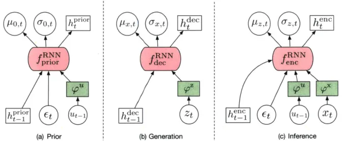
VRNN is a recurrent generative model used for modeling multi-modal trajectories. It has six interconnected components: a feature extractor for input :r, a feature
prior dec
h-1
(a) Prior (b) Generation
Figure 4-1: Illustrations for VRNN: (a) c generating xt using Eq 4.4; (c) updating h approximate posterior for zt using Eq 4.1.
[-tz't 9z't
fRNN enc
(c) Recurrence (d) Inference
)mputing conditional prior of zt using Eq 4.5; (b) idden RNN state ht using Eq 4.12; (d) inference of
extractor for latent state pz, a prior prior, an encoder ,enc, a decoder odec and a RNN fRNN. Suppose we represent a given trajectory as (Xt) -1. During training, the encoder takes the trajectory as input and infers latent random variables (zt) as
(4.1) (4.2)
P(zt IXt) = e(p2,),
h,t),
[pz,,, I z,t] = ,,n" ( Px(xt), ht_ 1),
where Oen represents the encoder, Sox is a function that extracts features of xt, and
h is the hidden vector in the GRU. We then sample the latent random variable
from the above distribution using a reparameterization trick [27], formulated as Zt = 1
z,t + Et X Crt where et ~ .A(O, I). After that, the decoder uses the sampled latent variable zt to reconstruct the trajectory, following
(4.3)
where
[yxt, Cx,1] = ,dec(z(zt), h_1). (4.4)
Here, W dec is the decoder and Sz is a feature extractor for zt.
In a VAE, we enforce the distribution of the latent vector (zt) to be close to a prior
34
fRNN U htReurn (c) Recurrence Iz,t 0z,t enc PU Ox ht-1 Xt (d) Inference
Figure 4-2: Illustrations for conditional
Eq 4.11; (b) generating Xt using Eq 4.4;
VRNN: (a) computing conditional prior of zt using (c) updating hidden RNN state ht using Eq ??; (d) inference of approximate posterior for zt using Eq 4.9.
distribution [27]. In a VRNN, the prior prior is learned and follows the distribution
P(zt) = A(piot, Uo,t), where [ptot, Jo,t] = ,prior(ht_ 1). (4.5)
Finally, the RNN fRNN updates its state as
(4.6)
The VRNN is trained by minimizing
EDK (JV(Pz,t, Uz,t|I|I(PO,t,
rO,0))
t=1- EZ P P(xtpz,t + Ei,t x or,t) + A1101|2,
t=1 i=1
(4.7)
where es,t - K(O, I), A is a regularization constant, and 0 is a vector containing all
the parameters in our model.
Once the VRNN is trained, we use the prior to sample latent random variables and use them to generate trajectories using the decoder and state update RNN. We ignore the encoder during test time.
po't UO't prior (a U (a) Prior Sdec Zt (b) Generation ht = f RNN (x p'(t) 2X) , ht -1).
4.2
Conditional VRNN
We want a VRNN to be conditioned on a sequence (ut)[- (e.g., the control inputs). Note that the distribution of xt is conditioned on ut_1. To this end, the posterior distribution of zt (Eqn. 4.1) is now
P(ztIxt, Ut1) = M(Pz,, I2,t), (4.8)
where
[p z,tl = ,enc(ox(xt), (ut- 1),1 ht_ 1). (4.9)
The prior distribution (Eqn. 4.5) also becomes conditional
P(ztlut_1) =Av(po,, Ot), (4.10)
where
[Po,t, t = _O prio(u(Ut-1), ht_ 1) (4.11)
And the state update equation (Eqn. 4.12) becomes
ht = f RNN p z) pu (t1,h-1.(.22(x(t
Here, the decoder (Eqn. 4.4) does not depend on (ut)[iJ because the latent vectors (zt)[1 already have the capacity to contain all information about the control sequence
T-1
(Ut)t=O1
Once the Conditional VRNN is trained, we use the prior to sample latent random variables and use them to generate trajectories using the decoder and state update RNN. We ignore the encoder during test time.
4.3
Decoupled Conditional VRNN
In our experiments, we predict trajectories whose length varies from 100 to 1000. Because training and evaluating a VRNN becomes slower with these long
fRNN prior dec dJ RNN J encjRNN
Sz U x
hdec Zt he t t Xt
(a) Prior (b) Generation | (c) Inference
Figure 4-3: Illustrations for decoupled conditional VRNN: (a) computing conditional prior of
zt using Eq 4.18; (b) generating xt using Eq 4.16; (c) inference of approximate posterior for zt using Eq 4.14.
ries, we propose an approximation to conditional VRNN, which we call Decoupled
Conditional VRNN. A conditional VRNN is slow, because updates in a RNN have
temporal dependence. However, we observe that the encoding, decoding, and prior networks are not inter-dependent: for example, the encoder only needs et to sample zt internally; it does not take signals from the decoding and the prior networks. Thus, in DCVRNN, we disentangle the model into three recurrent neural nets, one each for priors, the encoder, and the decoder. Specifically, we first have the Gaussian noises sampled as et ~ A(0, I). Then the equation for the encoder becomes
(4.13)
where
h!", [en , - RNN (x (xt), ou(ut--)I et, h n) (4.14)
The decoder is now
(4.15)
where
P(xtlzt ) = JV( PX,, a-x,t),
htc, Wx 1 - RNN (z (zt), ht- (4.16)
The prior is now
P(zt Iuti) = A(po,t, U-o,t), (4.17)
where
htrir, [[Ot, = flN ro,t] Np(ut_ 1), Et, ht2ir). (4.18)
The loss function remains unchanged.
We use a DCVRNN as our stochastic data-augmented residual model by having
Xt = st, Ut = [so, at, t+1, .t+i = fp( t, at), (4.19) where st represents the state at time t, at represents the action at time t,
fp
representsthe prior model, and 9t represents the state predicted by the prior model.
Once the DCVRNN is trained, we use the prior to sample latent random variables and use them to generate trajectories using the decoder. We ignore the encoder during test time.
Chapter 5
Residual Learning with Object-based
Networks
In Chapter 4, we described one way to realize the stochastic recurrent data-augmented residual model using GRU and then embed a conditional variational autoencoder in the GRU to make the model stochastic. But the final model, Decoupled Conditional VRNN, assumes a fixed number of objects in the world states. Thus it cannot be applied to states with a varied number of objects or generalize what it learns for one object to other similar ones.
To address this problem, rather than using the GRU as a building block for residual model, we use interaction networks
[3].
It is a graph-structured network model which is effective at generalizing over objects, modeling interactions, and handling variable numbers of objects. We extend the interaction network to make multi-step prediction and embed a conditional variational autoencoder in it to incorporate stochasticity.5.1
Interaction Network
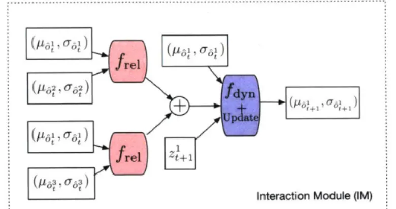
An interaction network consists of 2 neural nets: fdyn and frei. The frei network calculates pairwise interactions between objects and the fdyn network calculates the next state of an object, based on the states of the objects it is interacting with and the nature of the interactions.
The original version of interaction network was trained to make a single-step prediction; for improved accuracy, we extend them to make multi-step predictions. Let st = {ol, o,..., o} be the state at time t, where o' is the state for object i at time t. Similarly, let
st
={6,2,
... , 5n} be the predicted state at time t where o' is the predicted state for object i at time t. In our work, o' = [p', vT, mT, r'] where p' isthe pose of object i at time step t, v the velocity of object i at time step t, m' the mass of object i and r' the radius of object i. Similarly, ' = [pi, m', r'] where P' is
the predicted pose of object i at time step t and
i4
the predicted velocity of object i at time step t. Note that we do not predict any changes to static object properties such as mass and radius. Also, we note that while st is a set of objects, the state of any individual object, o', is a vector. Now, let a" be the action applied to object i at time t.The equations for the interaction network are:
Zfri tp -pt,v' - vj, m', mi, r', r), (5.1)
1= v' + dt x fdy (v, at, m2, rl, et), (5.2)
= p" + dt x E (5.3)
t+1= [ +1,+ 1,m2,r]. (5.4)
These equations describe a single-step prediction. For multi-step prediction, we use the same equations by providing the true state so at t = 0 and predicted state
st
at t > 0 as input. The interaction network can be trained by minimizing the mean squared error between the true object states and the predicted object states.5.2
Simulator-Augmented Interaction Networks
A simulator-augmented interaction (SAIN) network extends an interaction network, where fdyn and frei now take in the prediction of a prior model,
f,.
We now learn the residual between the prior model and the real world. Let st ={61,
62, . .}
be theOt 011
®
rel 0 2 t fdyn 01 Uplate O rel a' -1 ot+1 11 Ot frel t+1 t 020 Ot fdyn 01 -1 tt Ua t frel Ot(a) Interaction Networks (IN) (b) Simulator Augmented Interaction Networks (SAIN)
Figure 5-1: (a) Interaction network (IN) applied to object 1 in an environment with 3 objects
using Eq 5.1 (b) Simulator Augmented Interaction network (SAIN) applied to object 1 in an environment with 3 objects using Eq 5.5.
state at time t and 6' be the state for object i at time t predicted by the prior model. The equations for SAIN are
9t+1 et t?+1 O 1 = fp(t, a , a , ... , n) = frei(Vt, +i - ), p -y P J - , m , I = Vz + dt x fdyn(V V +1, a , m, rZ, ez), = p + dt x t+1 [+ 1iNt+, mI, r ]. (5.5) (5.6) (5.7) (5.8) (5.9)
These equations describe a single-step prediction. For multi-step prediction, we use the same equations by providing the true state so at t = 0 and predicted state At at t > 0 as input. The SAIN can be trained by minimizing the mean squared error between the true object states and the predicted object states.
frel t
t t fdyn
Updat
frel t+ 1
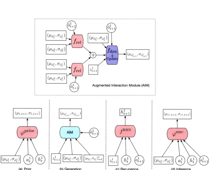
Interaction Module (IM)
t+ (/LlI~ I ztl
prior M RNN enc
(a) Prior (b) Generation (c) Recurrence (d) Inference
Figure 5-2: Illustrations for SIN applied to object 1 in an environment with 3 objects: (a) computing conditional prior of z+1 using Eq 5.20; (b) generating o+1 using Eq 5.12; (c)
updating hidden RNN state ht+1 using Eq 5.22; (d) inference of approximate posterior for
zt+1 using Eq 5.10.
5.3
Stochastic Interaction Network
A stochastic interaction network (SIN) combines an interaction network with a
con-ditional VRNN (CVRNN). The initial motivation for using decoupled concon-ditional VRNN (DCVRNN) was that CVRNN was slow. In practice, we observed that com-bining interaction network with either CVRNN or DCVRNN yielded similar speed because the interaction network was the slowest component. Therefore, we chose to combine interaction network with CVRNN, since DCVRNN is just an approximation of CVRNN.
Just like CVRNN, SIN has 3 major components: prior, encoder and decoder. The decoder contains the interaction network. Furthermore, given its stochastic nature,
SIN maintains a distribution over future states rather than a point estimate. 42
Let st {oI, o,..., o } be the state at time t, where o' is the state for object i at time t. Let pgt {pi, /161 . [ ., .
}
be the mean of the predicted state at timet, where p/35 is the mean of the predicted state for object i at time t. Similarly, let
= {3,-, . . . ,t
}
be the variance of the predicted state at time t, where o-3 is thevariance of the predicted state for object i at time t. In our work, p,5i [-pi, /pbi, i2, ri
where ppi is the mean of the predicted pose of object i at time step t, pji the mean of the predicted velocity of object i at time step t, mi the mass of object i and r' the radius of object i. Note that we do not predict any changes to static object properties such as mass and radius and therefore, don't maintain any variance over these properties. Similarly, c-a =
[-,
o-]j where o- is the variance of the predicted pose of object i at time step t and a-i the variance of the predicted velocity of objecti at time step t. Also, we note that while st is a set of objects, the state of any
individual object, ot, is a vector. Now, let a' be the action applied to object i at time t. Now we describe the three main components of SIN. Let Et - A,(0, I) be the sampled
gaussian noise. Then the equation for encoder becomes
P(z'+1 I o+,, a') = AN(pzi,t21, o-zi,t, 1 (5.10)
where
[Pzi,t+1, Ol24,t+1] = , (Vti+ , Pyi, (^fi, a ,mi, re, hi). (5.11)
We then sample the latent random variable from the above distribution using the reparameterization trick, formulated as z+ 1 zi,t+1 + ct x azi,t+I where Et ~ (, I).
Now the decoder uses the sampled latent random variable to reconstruct the trajectory. The interaction network is embedded within the decoder.
where e = frel (pj , -Q p /-tp , b p , m m i rI, r) [pT+ 11, O~+ +1 fdyn (e
,
j, ei -r p = + dt -p 1 00 o + dt2 .0. + -pi = ppi + dt - pi I S = pi + dt2 .y I~e A3' [-Pi ) Pf , m r ],P0i = [OI )Mi],
03 = 0pv, , O-i 0. 0 (5.13) (5.14) (5.15) (5.16) (5.17) (5.18) (5.19)
Note that the decoder does not depend on (a')_-' because the latent vectors
(zt)_1
already have the capacity to contain all information about the control sequence (at i_-. The prior distribution becomes
(5.20)
where
(5.21)
[pit, u~~+1] = (p oi , at, mz, r, ht). The state update equation becomes
+1= fRNN +1 t+1mi ri h) (5.22)
44
The SIN is trained by optimizing
n T
E DKL
(A
(pzit,7 o- I t I | (pi,t , 0-it))n T L
E~ E3 E3 ~3P(ol/Izj,t + ci,t x o-2i,t) + AI161, j=1 t=1 i=1
where ei,t ~ .A(O, I), A is a regularization constant, and 0 is a vector containing all the parameters in our model.
Once the SIN is trained, we use the prior to sample latent random variables and use them to generate trajectories using the decoder and state update RNN. We ignore the encoder during test time.
5.4
Stochastic Simulator-Augmented Interaction
Net-works
Similar to SIN, a stochastic simulator-augmented interaction (SSAIN) combines SAIN with CVRNN. It has 3 major components: prior, encoder and decoder and it differs from SIN only in terms of decoder. Its prior and encoder are same as those of SIN. It can be trained using same loss as SIN.
We will use the notation introduced in last section. Let 9t = {j, C1 , .. . , } be the state at time t and 6t be the state for object i at time t predicted by the prior model. The equations for the decoder are
6++ pA +1
frei i
tU t
frel
(IL,3 O ),
-1 Augmented Interaction Module (AIM)
5t1
pprior AIM RNN
() Pro ( t ( c) (Recurren
(a) Prior (b) Generation (c) Recurrence
enc
( ) aI h O+
(d) Inference
Figure 5-3: Illustrations for SSAIN applied to object 1 in an environment with 3 objects: (a) computing conditional prior of z+1 using Eq 5.20; (b) generating ot+1 using Eq 5.23; (c)
updating hidden RNN state ht+1 using Eq 5.22; (d) inference of approximate posterior for
zt+1 using Eq 5.10.
where
st1 =fp ( t, a , I f .. ., n,),
.= frel(fil - Vi, Vbi, 0~b, Ppi - Ppi, [4i - Ly , mi, mT, r, r) ji
[p +1i,, ort+11 = fdyn(Vt+1Ii ei,bi, I Z +17 M rI
Ipt 1 = p
+
dt xp 1,j = -+
dt2 x 1, (5.24) up = pi +dt x p, (5.25) r, o- + dt2 X O-, (5.26) 6+1 [ +1 , +1 y m ri], (5.27) 3 = [o- i ,o ,(5.28) /13i = [P , IV, Im I r ],(5.29) Cro = 0. (5.30)Note that the decoder does not depend on (a i)7i because the latent vectors (zf_[ 1
already have the capacity to contain all the necessary information about the control sequence (a i)_o.
Once the SSAIN is trained, we use the prior to sample latent random variables and use them to generate trajectories using the decoder and state update RNN. We ignore the encoder during test time.
Chapter 6
Control with Object-based Neural
Networks
Our action space has two free parameters: the point where the robot contacts the first disk and the direction of the push. In our experiments, a successful execution requires searching for a trajectory of about 50 actions. Due to the size of the search space, we use an approximate receding horizon control algorithm with our dynamics model. The algorithm remains the same whether we use SAIN or stochastic SAIN but the cost that the algorithm is optimizing changes. The search algorithm maintains a priority queue of action sequences based on the loss introduced below.
6.1
Control Algorithm for SAIN
For each expansion, let st be the current state and
st+T(at,
... , at+T-1) be the predicted state after T steps with actions at,. .. , at+T-1. Let s9 be the goal state. We choosethe control strategy at that minimizes the the cost function
St+T(st, at, ... , at+T-1) - Sg 12 and insert the new action sequence into the queue.
strategy is incomplete in general and wouldn't work if the control task has certain complexities like presence of obstacles. But since we don't have any such complexity in our task, a greedy strategy is enough to find a control strategy.
6.2
Control Algorithm for SSAIN
For each expansion, let st be the current state and pg+, (at, ... , at+T-1) and O-9+T (at, ... , at+T-1)
be the mean and the variance of the predicted state after T steps with actions
at,..., at+T-1. Let s9 be the goal state. We choose the control strategy at that minimizes the the cost function
(Ipt+T (st, at, ... , at+T-1) - sg) OAt+T (at,. .. , at+T-1) (PIt+T (St, at, ... , at+T-1) - s)+
A log(det(aOrk+(at,... , at+T-1)))
and insert the new action sequence into the queue. Here A is the regularization constant.
We explain the control strategy in details later in subsection 7.3.2. The greedy strategy is incomplete in general and wouldn't work if the control task has certain complexities like presence of obstacles. But since we don't have any such complexity in our task, a greedy strategy is enough to find a control strategy.