HAL Id: hal-00349278
https://hal.archives-ouvertes.fr/hal-00349278
Submitted on 13 Jan 2016
HAL is a multi-disciplinary open access
archive for the deposit and dissemination of
sci-entific research documents, whether they are
pub-lished or not. The documents may come from
teaching and research institutions in France or
abroad, or from public or private research centers.
L’archive ouverte pluridisciplinaire HAL, est
destinée au dépôt et à la diffusion de documents
scientifiques de niveau recherche, publiés ou non,
émanant des établissements d’enseignement et de
recherche français ou étrangers, des laboratoires
publics ou privés.
processing across the North Atlantic
Elsa Real, Kathy S. Law, H. Schlager, Anke Roiger, H. Huntrieser, J.
Methven, M. Cain, J. Holloway, J.A. Neuman, T. Ryerson, et al.
To cite this version:
Elsa Real, Kathy S. Law, H. Schlager, Anke Roiger, H. Huntrieser, et al.. Lagrangian analysis of
low altitude anthropogenic plume processing across the North Atlantic. Atmospheric Chemistry and
Physics, European Geosciences Union, 2008, 8 (24), pp.7737-7754. �10.5194/acp-8-7737-2008�.
�hal-00349278�
www.atmos-chem-phys.net/8/7737/2008/ © Author(s) 2008. This work is distributed under the Creative Commons Attribution 3.0 License.
Chemistry
and Physics
Lagrangian analysis of low altitude anthropogenic plume processing
across the North Atlantic
E. Real1,*, K. S. Law1, H. Schlager2, A. Roiger2, H. Huntrieser2, J. Methven3, M. Cain3, J. Holloway4, J. A. Neuman4, T. Ryerson5, F. Flocke6, J. de Gouw4, E. Atlas7, S. Donnelly8, and D. Parrish5
1Service d’A´eronomie/UPMC, CNRS-IPSL, 4 Place Jussieu, 75005 Paris, France
2Deutsches Zentrum f¨ur Luft- und Raumfahrt (DLR), Oberpfaffenhofen, Institut f¨ur Physik der Atmosph¨are,
82230 Wessling, Germany
3Department of Meteorology, University of Reading, P.O. Box 243, Earley Gate, Reading, RG6 6BB, UK 4NOAA ESRL/CIRES, University of Colorado at Boulder, Boulder CO 80309, USA
5NOAA ESRL, 325 Brodway, Boulder, CO 80305 USA
6Atmospheric Chemistry Division, NCAR, 1850 Table Mesa Drive Boulder, CO 80305 USA 7RSMAS/MAC University of Miami, Miami, FL 33149 USA
8Department of Chemistry, Fort Hays State University, Hays KS 67601 USA *now at: CEREA, Paris Est, 20 rue Alfred Nobel 77455, Champs sur Marne, France
Received: 12 March 2008 – Published in Atmos. Chem. Phys. Discuss.: 17 April 2008 Revised: 24 November 2008 – Accepted: 24 November 2008 – Published: 23 December 2008
Abstract. The photochemical evolution of an anthropogenic
plume from the New-York/Boston region during its transport at low altitudes over the North Atlantic to the European west coast has been studied using a Lagrangian framework. This plume, originally strongly polluted, was sampled by research aircraft just off the North American east coast on 3 succes-sive days, and then 3 days downwind off the west coast of Ireland where another aircraft re-sampled a weakly polluted plume. Changes in trace gas concentrations during transport are reproduced using a photochemical trajectory model in-cluding deposition and mixing effects. Chemical and wet de-position processing dominated the evolution of all pollutants in the plume. The mean net photochemical O3production is
estimated to be −5 ppbv/day leading to low O3by the time
the plume reached Europe. Model runs with no wet deposi-tion of HNO3predicted much lower average net destruction
of −1 ppbv/day O3, arising from increased levels of NOxvia
photolysis of HNO3. This indicates that wet deposition of
HNO3is indirectly responsible for 80% of the net destruction
of ozone during plume transport. If the plume had not en-countered precipitation, it would have reached Europe with
Correspondence to: E. Real
O3concentrations of up to 80 to 90 ppbv and CO between
120 and 140 ppbv. Photochemical destruction also played a more important role than mixing in the evolution of plume CO due to high levels of O3and water vapour showing that
CO cannot always be used as a tracer for polluted air masses, especially in plumes transported at low altitudes. The results also show that, in this case, an increase in O3/CO slopes can
be attributed to photochemical destruction of CO and not to photochemical O3production as is often assumed.
1 Introduction
It is recognised that emissions from large urban/industrial re-gions can have large-scale impacts on concentrations of O3,
particles, and other trace constituents downwind from conti-nents. These impacts are important because they may affect the ability of downwind countries to meet air quality stan-dards, and because of climate impacts of O3 and particles
through radiative forcing. Anthropogenic pollution occurs primarily in the boundary layer (BL) over continents. This pollution may then be transported at low levels directly im-pacting the BL of a downwind continent or may be exported from the BL into the mid and upper troposphere by frontal systems or convection and transported at higher altitudes (Li
et al., 2005). Because of lower water vapour and temper-ature, loss processes are less active and pollutant lifetimes longer in the upper troposphere. However, high altitude plumes are less likely to directly impact the BL composition of a downwind continent. Several modelling studies have already shown that long-range transport of pollutants from North America to Europe is one of the most important due to large emissions and the relative proximity of the two con-tinents (Wild and Akimoto, 2001; Stohl, 2001; Stohl et al., 2002). There is clear experimental and modelling evidence for such export from North America at both low and high altitudes. Polluted plumes have been sampled at remote sur-face sites such as Sable Island or Chebogue Point (Parrish et al., 1998; Millet et al., 2006), off the New England coast, and also downwind in the Azores (Parrish et al., 1998; Owen et al., 2006) in the mid-Atlantic Ocean. Analysis of these polluted plumes showed that they were usually transported at low altitudes, below 3 km. Modelling studies suggest that one third of CO exported from North America occurs in the lowest 3 km (Li et al., 2005) and Owen et al. (2006) sug-gested that low level transport of North American pollution above the marine BL may provide an effective mechanism for long-range transport of anthropogenic pollution over the North Atlantic with a resulting impact on lower tropospheric O3in downwind regions.
Whilst there have been several measurements of polluted plumes with North American origins in the free troposphere over Europe (e.g. Huntrieser et al., 2005), there have been fewer detailed cases at low levels and the impact of such long-range transport on O3 levels in the European BL is
not well documented (Derwent et al., 1998). Ground-based sites on the west coast of Europe do occasionally observe such cases. For example, Li et al. (2002) reported sev-eral measurements of moderately polluted plumes at Mace Head (west coast of Ireland) with weak enhancements in CO and O3. Despite the relative lack of experimental evidence,
global model simulations suggest that the impact of anthro-pogenic North American pollution on European BL O3 is
important. Li et al. (2002) and Auvray and Bey (2005) es-timated an increase of 2 to 4 parts per billion by volume (ppbv) in European O3concentrations during summer, which
could be responsible for 20% of the violation of the European Union threshold for O3. These studies suggest that half of
the import of North American O3in the BL is due to
trans-port at low altitudes with the remainder due to subsidence of high altitude plumes. Derwent et al. (2004) suggested a higher value of 8 ppbv increase in the European BL using an O3tracer technique in a semi-Lagrangian global model.
During high pollution events, under conditions typified by a strong Icelandic Low located between Iceland and the British Isles, Auvray and Bey (2005) simulated an increase in Eu-ropean O3 due to North American pollution of more than
than 10 ppbv. Several explanations have been proposed for the difference between the non-negligible impact of North American pollution on European O3 simulated by models
and the lack of experimental evidence. Stohl et al. (2002) suggested that North American pollution reaches the Euro-pean BL primarily south of the Pyrenees where measure-ment sites are sparse, and also that North American plumes are generally older then 10 days when reaching Europe, and therefore, hard to accurately trace back to sources.
In this study, we address these issues through the analysis of data collected in a pollution plume transported at low alti-tudes over the North Atlantic as part of the International Con-sortium for Atmospheric Research on Transport and Trans-formation (ICARTT) (Fehsenfeld et al., 2006) also encom-passing the European Intercontinental Transport of Ozone and Precursors (ITOP) experiment, which took place in sum-mer 2004. As part of this campaign, the International Trans-port and Chemical Transformation (ITCT) Lagrangian 2K4 experiment (an International Global Atmospheric Chemistry (IGAC) task) executed a Lagrangian study of polluted air masses transported across the North Atlantic. Four research aircraft based in North America, the Azores and western Europe sampled the same air masses several times during long-range transport. Lagrangian experiments have been conducted previously, but this was the first time that a La-grangian experiment was conducted in the free troposphere on intercontinental scales. The main advantage of this kind of study is that changes in plume concentrations over several days can be estimated by comparing two Lagrangian sam-plings, and the processes leading to these changes can be evaluated with reduced uncertainty. After the campaign a detailed analysis using trajectories, a Lagrangian dispersion model, and in-situ measurements was performed by Methven et al. (2006), and showed that there were five cases where the same air mass had been sampled several times across the At-lantic.
The overall goal of this paper is to improve our under-standing about low altitude long-range transport of anthro-pogenic plumes over the North Atlantic and their impact on O3and precursors levels over Europe. In particular, we
anal-yse the evolution of a North American plume observed dur-ing the Lagrangian 2K4 experiment which was originally very polluted, and then transported at low levels over the North Atlantic toward Europe. The aim is also to determine the relative importance of processes influencing its chemical composition, and to explain why polluted North American plumes are not easily detected at surface measurement sites in Europe.
The Lagrangian plume in question originated from the New York-Boston conurbation and was sampled 3 times just off the New England coast on 3 successive days by the Na-tional Oceanic and Atmospheric Administration (NOAA) P3, and then, 2 days later off the west coast of Ireland, and 3 days later over the English Channel by the German Deutsches Zentrum fur Luft- und Raumfahrt (DLR) Falcon. First, the Lagrangian matches identified by Methven et al. (2006) are discussed in Sect. 2 together with the observed chemical evo-lution of pollutants during the plume transport. Cases where
the Lagrangian matching is less good due to the influence of other processes such as mixing with local emissions are also identified. Next, to evaluate the relative contributions of chemical, physical and dynamical processes to changes in O3
concentrations in the plume during transport, a photochem-ical trajectory model was used (Sect. 3). In Sect. 4, results are presented from model runs initialised with upwind data over New England, and compared to downwind data over Eu-rope. The model was run along a trajectory representative of the mean plume transport pathway and giving the best match between plume samplings. The model was first run with chemistry only (Sect. 4.1), and then including wet and dry deposition (Sect. 4.2). The sensitivity of the results to het-erogeneous loss on aerosols was also analysed. The impact of mixing with air masses in close proximity to the plume is examined in Sect. 4.3. The ability of the model to simulate the contribution of photochemical processes to O3 changes
in the plume was further tested by examining the evolution of trace gas correlations using multiple model runs initialised across the first plume sampling (Sect. 4.4). Conclusions are presented in Sect. 5.
2 Lagrangian case: measurements and analysis
2.1 Identification of Lagrangian matches
Methven et al. (2006) used a novel technique to identify La-grangian matches between flight segments from different air-craft during the entire IGAC Lagrangian 2K4 experiment in July 2004. This technique combined trajectories, calculated using global meteorological analysis (European Centre for Medium Range Weather Forecast 40 year Reanalysis – ERA-40), and hydrocarbon fingerprint analysis. A match was de-fined as an occasion when a pair of whole air samples (anal-ysed for their hydrocarbon content) collected during different flights exhibited highly correlated hydrocarbon fingerprints (when such measurements were available), and the sample time windows were also connected by both backward and forward trajectories. Results from the Lagrangian particle dispersion model, FLEXPART, run with CO tracers (Stohl et al., 2004) were also used to confirm matches. Five clear Lagrangian cases covering a variety of situations were iden-tified. Further details can be found in Methven et al. (2006). In this paper, we build on the work of Real et al. (2007) which focused on the Lagrangian analysis of the long-range transport of a forest fire plume during ICARTT, one of the cases discussed by Methven et al. (2006). Here, we examine another case from Methven et al. (2006) where an anthro-pogenic pollutant plume was transported across the North Atlantic at low altitudes. The plume from the New York-Boston region was first sampled by the NOAA P3 over the Gulf of Maine and Nova Scotia on 3 successive days (20, 21, 22 July), and then by the DLR Falcon flying just off the coast of Ireland on 25 July and over the English
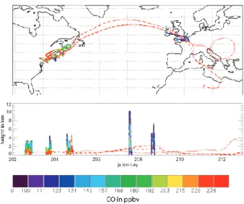
Chan-Fig. 1. Flight tracks of P3 flights on 20, 21, and 22 July 2004
and Falcon flights on 25 and 26 July 2004, coloured with measured CO. Three forward trajectories initialised in the 3 Lagrangian sam-plings of the P3 are also shown for 20 (dotted), 21 (dashed) and 22 (dashed-dotted) July 2004, respectively.
nel on 26 July 2004. The flight tracks of these 5 flights are shown in Fig. 1. The segments of the 3 flights identified as Lagrangian matches were labelled as Lagrangian case 3 by Methven et al. (2006). The same Lagrangian time windows are used in this study. The ability of the Methven et al. (2006) analysis to identify Lagrangian matches has been shown to work well in the free troposphere where transport is mainly driven by advection (Real et al., 2007). However, at low al-titudes, certain meteorological features are not so well re-solved by analysed winds, and can induce errors in the La-grangian analysis. For example, Riddle et al. (2006) analysed the ability of trajectory models to represent air mass trans-port during the ICARTT campaign by using Lagrangian bal-loons released over north-east North America. Balbal-loons were launched close to the Lagrangian match of the NOAA-P3 air-craft on 20 July. On 21 July, the balloon location and airair-craft Lagrangian match were very well co-located (less than 2 km apart) suggesting that the matching between these 2 samples is good. This is not the case for 22 July where the balloon was located far from the Lagrangian match. Indeed, im-portant differences were found between balloon and model trajectories between 21 and 22 July over the Newfoundland coast, possibly due to poor simulation of strong coastal winds in the ECMWF analyses. Also, hydrocarbon matches on 22 July were the least consistent (with increases in hydrocar-bon concentrations compared to the 2 previous days – see next section). Therefore, it appears that Lagrangian match between 20, 21 July and 22 July is less good. The accu-racy of the Lagrangian samplings is examined further in the next section where the observations in the plume segments are discussed.
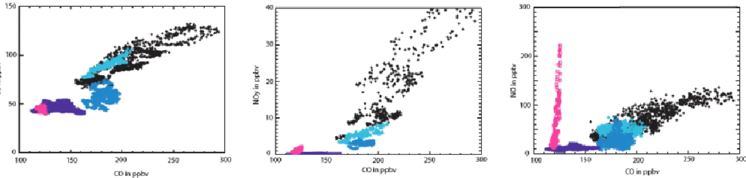
Fig. 2. Measured O3and reactive nitrogen concentrations (NO, NOy) versus measured CO in the 5 Lagrangian match samplings. Black
crosses represent measurements taken on 20 July and light blue triangles, dark blue diamonds, violet stars and pink squares the measurements taken on 21, 22, 25 and 26 July 2004, respectively.
22 July 20 July
25 July
Fig. 3. Infrared images combined from GOES and METEOSAT for
20, 22 and 25 July 2004 taken from the NOAA products in support of ICARTT (courtesy O. Cooper, NOAA ESRL). Black lines are surface pressure (hPa) and black crosses represent the location of the Lagrangian matches on each day.
The meteorological situation during plume transport has been examined using the Geodetic Earth Orbiting Satel-lite GOES-1 and METEOSAT satelSatel-lite images superimposed with surface pressure values (see Fig. 3). On 19 July, a cold front passed over the north-east coast of the United States (US). Behind this front, strong outflow took place below 3 km transporting air from the New York-Boston region on 20 July towards Newfoundland on 22 July. From the 22 to 25 July, strong winds established over the Atlantic Ocean be-tween the Azores/Bermuda High and the Icelandic Low, par-ticularly on 22 July, which transported the polluted plume to Europe. On 25 July the Icelandic Low moved northward allowing the air masses to reach the Irish coast. This low level export from the North American east coast in conjunc-tion with a cold front is a classical feature of North Amer-ican summertime meteorology, and has been shown by, for example, Li et al. (2005) to be an important factor driving summertime pollution export. Warm conveyor belts asso-ciated with cold fronts lift pollution from the central and north-eastern US into the free troposphere over Newfound-land, and strong north-eastward outflow takes places at low levels behind the cold front. Li et al. (2005) evaluated the occurrence of such events to be 5 to 7 per month in sum-mer. The transport over the North Atlantic towards Europe is then dependent on the position and strength of the Azores High/Icelandic Low. Guerova et al. (2006) reported that of the export events identified by Li et al. (2005), 3 reached cen-tral Europe, with about half at low altitudes. Li et al. (2002) evaluated a higher frequency of low level North American plumes reaching Europe during summer 1994 to 1997. The plume studied here is a case of this kind of pollutant export. 2.2 Chemical composition of the Lagrangian plume
matches
Detailed information about the instrumentation on board the aircraft can be found in Fehsenfeld et al. (2006). Since mea-surements taken by the different aircraft will be used to in-fer the chemical evolution of the plume, it is important to
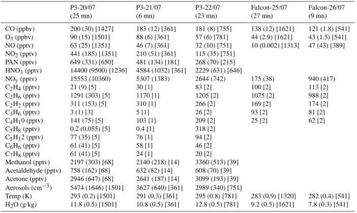
Table 1. Measurements taken during Lagrangian match windows (given in minutes (mn)) as defined in Table 1 of Methven et al. (2006).
Data for each window is shown as mean (standard deviation) [number of measurement averaged]. NOy values indicated for the first 3
Lagrangian matches are the sum of measured HNO3, PAN, NO2and NO. All measurements indicated in the first column (20 July) are used
to initialise the model, except for temperature, water vapour (taken from ECMWF meterological analyses) and aerosol concentrations (see text for details).
P3-20/07 P3-21/07 P3-22/07 Falcon-25/07 Falcon-26/07 (25 mn) (6 mn) (23 mn) (27 mn) (9 mn) CO (ppbv) 200 (30) [1427] 183 (12) [361] 181 (8) [755] 138 (12) [1621] 121 (1.8) [541] O3(ppbv) 90 (15) [1501] 88 (6) [361] 57 (6) [781] 44 (2.9) [1621] 43 (1.5) [541] NO (pptv) 63 (25) [1351] 46 (7) [361] 32 (10) [751] 10 (0.002) [1313] 47 (43) [389] NO2(pptv) 441 (185) [1351] 210 (51) [361] 115 (35) [751] PAN (pptv) 649 (331) [650] 481 (134) [181] 268 (70) [215] HNO3(pptv) 14400 (9500) [1236] 4584 (1032) [361] 2229 (631) [646] NOy(pptv) 15553 (10360) 5307 (1383) 2644 (742) 175 (38) 940 (417) C2H4(pptv) 21 (9) [5] 30 [1] 83 [2] 100 [2] 113 [2] C2H6(pptv) 1291 (303) [5] 1170 [1] 1205 [2] 1075 [2] 988 [2] C2H2(pptv) 311 (153) [5] 310 [1] 266 [2] 169 [2] 174 [2] C3H6(pptv) 3 (1) [3] 5 [1] 26 [2] 93 [2] 81 [2] C4H10 (pptv) 141 (75) [5] 103 [1] 209 [2] 25 [2] 62 [2] C5H8(pptv) 0.2 (0.055) [5] 0.4 [1] 318 [2] C5H12 (pptv) 77 (35) [5] 76 [1] 94 [2] C6H6(pptv) 61 (41) [5] 58 [1] 46 [2] C7H8(pptv) 61 (41) [5] 24 [1] 20 [2] Methanol (pptv) 2197 (303) [68] 2140 (218) [14] 3360 (513) [39] Acetaldehyde (pptv) 758 (162) [68] 632 (82) [14] 608 (70) [39] Acetone (pptv) 2946 (647) [68] 2641 (187) [14] 3099 (193) [39] Aerosols (cm−3) 5474 (1646) [1501] 3627 (640) [361] 2989 (340) [751] Temp (K) 293 (0.2) [1501] 291 (0.3) [361] 295 (0.8) [781] 283 (0.9) [1320] 282 (0.4) [541] H2O (g/kg) 11.8 (0.5) [1501] 10.8 (0.5) [361] 12.8 (0.5) [781] 9.2 (0.5) [1621] 7.8 (0.3) [541]
compare these measurements. Several comparison flights were performed between the 4 aircraft involved in the cam-paign. Overall, the comparison showed that O3
measure-ments agreed within 2 ppbv and CO within 3 ppbv, for the aircraft used in this study. Comparison of hydrocarbons was more difficult but, where possible, comparison showed good agreement. More details about the comparison flights can be found in Methven et al. (2006) and Fehsenfeld et al. (2006). The general behaviour of the plume evolution is first exam-ined in terms of observed trace gas mean values and corre-lations. Observed concentrations of O3, NO and NOy with
respect to CO in the 5 Lagrangian matches are shown in Fig. 2 with average values during the 5 match time windows reported in Table 1. Correlation coefficients, r, and slopes were also calculated and provide information about the dis-persion of data around the correlation line, and therefore, the quality of the correlation. These results are discussed later in Sect. 4.4 when they are compared to model simulations. (see Table 4).
The first interception of the plume by the P3 on 20 July showed a highly polluted plume with high values of CO (200 ppbv) very well correlated (r=0.91) with high values of O3 (90 ppbv), NOx (500 pptv) and very high levels of
NOy (15 550 pptv). Here, NOy was mainly in the form of
HNO3 representing approximately 92% of total NOy. One
day later, CO, O3and NOxlevels slightly decreased, but
re-mained elevated. HNO3concentrations showed the strongest
decrease to only 32% of the initial value. O3 and CO were still highly correlated with a similar slope (0.51) whereas the slope between NO and CO decreased strongly even though the two species were still very well correlated (r=0.85). On 22 July, CO, NOx, PAN, HNO3and O3levels decreased and
the species are not correlated any more with value of r be-tween 0.14 and 0.3. Moreover, concentrations of the main volatile organic compounds (VOCs) (C2H6, C2H4, C5H8,
CH3OH, acetone) increased and are higher than on the first
Lagrangian sampling. This lack of correlation, as well as the increase in VOCs, could be explained by strong and inhomo-geneous mixing with another air mass containing more recent emissions or, as discussed previously, this match appears to be incorrect due to large uncertainties in the calculation of trajectories on this day. Therefore, although comparisons be-tween model results and data on 22 July are shown, the un-certainty surrounding this match should be kept in mind.
The 3 North American interceptions (20, 21 and 22 July) were made close to remote surface sites in New England (Sable Island, Chebogue Point and Appledore Island). Pol-luted plumes from the New York-Boston region are often
encountered in this region, as shown by Chen et al. (2007) who estimated that these events occurred 15% of the time during summer 2004. Comparison of measurements in the Lagrangian match and those analysed by Parrish et al. (1998) at Sable Island and Chebogue Point between 1991–1994, shows that the mean O3and CO values as well as the O3/CO
measured slopes are in the upper range of the surface obser-vations. The aircraft observations were collected away from the surface and were probably subject to less dry deposition of O3. Another factor that can explain the larger O3/CO slope
is that the NOxto CO emission ratio in the US has changed
since the early 1990s. Assuming that the production of O3
is NOxlimited, then steeper O3/CO relationships could be
expected in 2004 as suggested by Honrath et al. (2004). After the plume crossed the North Atlantic it was in-tercepted on 25 July by the DLR Falcon aircraft off the west coast of Ireland. Lower concentrations of pollutants were measured with mean concentrations of 138 ppbv CO, 44 ppbv O3, and 175 pptv NOy, which represents only 2% of
the initial NOyvalue. Correlations between species are now
very low including the O3/CO slope (−0.03). Mean values
and slopes can be compared with those measured in North American plumes (identified using a global model) in sum-mer at Mace Head (53◦N, 10◦W), on the Irish west coast between 1994 to 1997 by Li et al. (2002). Whilst the aver-age values measured in the Lagrangian plume are within the normal measured range, the O3/CO slopes are much lower
than the values of 0.2 to 0.4 reported by Li et al. (2002). Rea-sons for the discrepancies between these measured slopes are analysed further in Sect. 4.4. Note that whilst the O3
concen-trations in the match on 25 July are much lower than in the first samplings of the plume, they still represent an increase compared to background in the remote marine environment where the measurements were taken, i.e. 10 to 20 ppbv above average for O3and 10 to 40 ppbv for CO.
According to Methven et al. (2006), the plume was inter-cepted a last time by the Falcon over the English Channel on 26 July with CO and O3 levels slightly lower than the
previous day and a negative O3/CO slope. As for NO and
NOy, concentrations are much higher compared to the
previ-ous match and NO and NOylevels were even higher than in
the first match. This suggests that strong mixing with freshly polluted European air masses may have taken place.
The evolution of this plume in terms of changes in ob-served concentration changes seems fairly typical with re-ductions in pollutant levels during transport across the At-lantic and in terms of transport by cold front advection over the US followed by rapid transport towards Europe. Further analysis using a photochemical trajectory model and compar-ison with measured concentrations in the Lagrangian match segments will provide an insight into the processes which are responsible for the evolution of pollutant levels in this plume.
3 Modelling
The Lagrangian photochemical model, CiTTyCAT (Cam-brIdge Tropospheric TrajectorY model of Chemistry And Transport) has been used to examine the different processes influencing the evolution of trace gases within the plume, and in particular, O3, CO and NOy. CiTTyCAT has been
used previsously to examine the origin of polluted layers over the North Atlantic during past campaigns (Wild et al., 1996; Evans et al., 2000). This model also successfully captured the evolution of trace gas concentrations over the North At-lantic in the ICARTT forest fire case identified by Methven et al. (2006) (Real et al., 2007). The model is considered as an isolated air parcel, and run along trajectories calculated using large-scale meteorological analyses. Ninety chemi-cal species are treated in the model including degradation of 14 hydrocarbons using chemical rate data from JPL (2003) and updates discussed in Arnold et al. (2006) for acetone and ethanol. The photolysis scheme used in the runs pre-sented here is based on a 2-stream multiple scattering scheme (Hough, 1988).
3.1 Chemical initialisation
First, the model was used to simulate the evolution of aver-age concentrations in the plume (Sects. 4.1, 4.2.1, 4.3). The model was initialised with concentrations measured in the plume on 20 July by the P3, and compared with average con-centrations measured by the same aircraft on 21 and 22 July as well as by the Falcon on 25 and 26 July. These measured concentrations are indicated in Table 1. The only specie for which the initial value has not be taken from measurements is methane, with a typical value of 1.8 ppmv. In order to charac-terise the variability in plume concentrations, 3 simulations were carried out: one using mean concentrations measured during the plume match segment on 20 July, and 2 others us-ing the mean concentrations + (−) standard deviation (std). Note that all species are well correlated in the plume mak-ing this approach appropriate. Then, in order to extend the analysis the model was initialised across the full range of concentrations in each match segment on 20 July and their inter-relationships (correlations) analysed (Sect. 4.4). 3.2 Trajectories
The model was run along a trajectory calculated with the FLEXTRA model (Stohl et al., 1995) using ECMWF ERA-40 wind fields. Position, temperature and water vapour used in CiTTyCAT were interpolated from the FLEXTRA trajec-tory at every CiTTyCAT time-step. All trajectories initialised in the P3 Lagrangian match on 20 July showed approxi-mately the same transport, so the one initialised around 21:20 was chosen (see Fig. 1). This trajectory passes closest to the P3 Lagrangian matches on 21 and 22 July, and the Falcon matches on 25 and 26 July.
pptv pptv pptv ppbv ppbv ppbv ppbv H2O in g/kg T in K
Concentrations, water vapour and temperature Hourly O3production and destruction terms
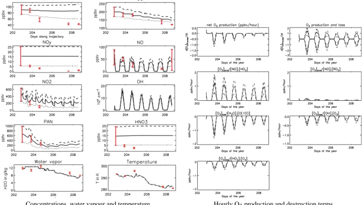
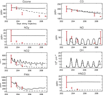
Fig. 4. Temporal evolution (Julian days) of (a) simulated concentrations, and (b) simulated O3production and destruction rates, initialised
with mean (continuous lines), mean – std (dotted line) and mean +std (dashed lines) concentrations taken from the P3 data during the match segments on 20 July. Downwind mean and std data observed during the plume match segments are represented as red vertical lines (see text for details).
3.3 Representation of physical phenomena
Wet and dry deposition as well as mixing can be included in the model. Dry deposition is simulated when the air par-cel is in the BL using a velocity parameter which depends on surface type and on the height of the BL. The BL was defined climatologically from GEOS-1 meteorological data (Schubert et al., 1993). The original wet deposition scheme is a simple scheme using a lifetime for soluble species. More details about the model can be found in Wild et al. (1996) and Evans et al. (2000). The model was first run with only pho-tochemical processes (Sect. 4.1) in order to study the chemi-cal evolution of the plume in the absence of other processes. Then, since the plume was transported at low altitudes, and sometimes in the BL, runs were made including dry deposi-tion (Sect. 4.2.1). GOES METEOSAT satellite images (see Fig. 3) indicate the presence of clouds, on certain occasions, in the same location as the plume, especially over the North American coast. Moreover, the strong decrease in HNO3
ob-served in the plume is likely to be the result of wet deposi-tion since HNO3is highly soluble. For this reason, runs were
also carried out including wet deposition. In addition, a new scheme was implemented based on precipitation rates from ECMWF (Sect. 4.2.2). Note that aerosol levels in the plume were high initially but dropped between 20 and 22 July from
about 5.5×10³particles per cm−3 to 3.0×103cm−3 which may also indicate that deposition was active, even if other mechanisms (dilution, coagulation) could also explain this decrease. Heterogeneous reactions were not included in the majority of simulations discussed here. However, the sensi-tivity of results to N2O5hydrolysis on aerosols was
exam-ined and is discussed in Sect. 4.2.3. Finally, mixing between the plume and surrounding air masses was also considered (Sect. 4.3).
4 Results
4.1 Chemistry-only simulations
Simulated concentrations of CO, O3, NO, NO2, HNO3and
PAN for the model runs initialised with mean, mean +std and mean −std concentrations measured in the P3 Lagrangian match on 20 July are shown in Fig. 4 together with simulated O3production and destruction terms. Water vapour and
tem-perature data interpolated along the trajectory from ECMWF analyses are also shown. These results include only changes due to photochemical processes in the model.
4.1.1 Simulated plume characteristics
The modelled chemical evolution of the plume shows two interesting features. Firstly, despite high levels of water vapour, high concentrations of NO, NO2, HNO3 and O3
are maintained in the plume whereas PAN levels decrease rapidly due to high temperatures. Analysis of O3
produc-tion and destrucproduc-tion terms shows that O3 destruction due
to water vapour is important, but is almost balanced by photochemical O3 production. Sensitivity tests will help
to understand the origin of this high O3 production (see
Sect. 4.1.3). The second interesting feature is the high oxidising capacity of the plume. In these chemistry only simulations, OH levels remain high during the entire run with mean values of 4×10⁶molecs. cm−3and peaks around 15×106molecs. cm−3around noon. This can be mainly ex-plained by high water vapour, due to the low altitude of the plume and high O3concentrations.
One of the main impacts of this high oxidising capacity is the strong photochemical destruction of CO, which decreases by about 50 ppbv in 6 days. CO is often considered as a pollution tracer, not really affected by chemical loss over a period of 10 days or less, with a strong decrease in CO usu-ally attributed to dilution and mixing. Here, assuming no other loss processes, CO decreased by 25% solely as a re-sult of chemical destruction. This would imply that for this plume, transported at low altitudes, the CO chemical lifetime is about 20 days. This value can be compared with a value of 30 days for the global mean CO lifetime during summer. 4.1.2 Comparison of measured and simulated
concentra-tions
The general evolution of measured PAN and CO values are reproduced in the model solely with chemical processing suggesting an important role for photochemistry in this case although CO is still overestimated after 6 days and PAN data were only available from the P3. Measured NO and NO2
val-ues are generally overestimated by the mean simulations, and are more represented by the mean – std simulation. O3
val-ues are overestimated by more than 40 ppbv after 5 days but the strongest difference is found between simulated and mea-sured HNO3with average modelled concentrations 13 ppbv
higher after 3 days. These differences suggest that other pro-cesses such as deposition, heterogeneous loss on aerosols or mixing may also be important. Unfortunately, measurements of other species like H2O2or HCHO for the three P3 flights
were not available to provide further tests of the model re-sults discussed in the next sections. Concerning OH, model results are the same order of magnitude as those calculated by Warneke et al. (2004) using a box model initialised with measurements from a research ship along the New England coast, i.e. in the same region as the Lagrangian plume during the first 3 days, albeit at a lower altitude. However, the peak noon values simulated here are higher than those measured,
for example, in the Los Angeles basin by George et al. (1999) (7×10⁶molecs. cm−3), and by Ehhalt and Roher (2000) at a
rural German site (12×106molecs. cm−3). Measured JO1D
and JNO2 during the 3 first Lagrangian samplings are in
good agreement with simulated values (not shown). In these chemistry only runs the model underestimates several VOCs: C2H2, C2H6, C4H10, C2H4and C3H6are underestimated by
70, 140, 20, 110 and 90 pptv respectively on the 25 July. Concerning water vapour and temperature, the difference be-tween measured values and those interpolated from ECMWF analyses along the trajectory is always less than 20% for wa-ter vapour and 4K for temperature. Therefore, in these runs which only take chemical processes into account, the overes-timation in O3leads to an overestimation in OH and therefore
other processes are also playing an important role as will be discussed in the following sections.
4.1.3 Sensitivity tests
In order to better understand photochemical processing in the plume and possible reasons for the differences between sim-ulated and observed O3, two sensitivity tests were performed.
Firstly, initial HNO3concentrations were reduced to zero
(S-noHNO3) in order to study the role of HNO3in the net
pro-duction of O3during transport. Secondly, a cloud with an
optical depth of 5 (value of the mean cloud optical depth observed globally by Rossow and Schiffer, 1991) was sim-ulated just above the plume (S-CLOUD) in order to exam-ine the maximum effect of a cloud layer on photolysis rates inside the plume. The S-CLOUD simulation is representa-tive of a maximum effect because clouds were not present during the entire transport over the North Atlantic as shown by the GOES-METEOSAT satellite images. In particular, clouds were not present during the match periods when, as noted previously, modelled photolysis rates agree well with the measurements. The chosen optical depth is also relatively high for non-convective clouds. In both cases simulations were initialised with mean values measured in the plume. Results of these sensitivity tests are shown in Fig. 5.
Results of the run S-noHNO3clearly show that the
main-tenance of high O3 levels in the chemistry-only simulation
is mainly due to HNO3photolysis. Indeed after 6 days, O3
concentrations in the S-noHNO3 simulation are lower than
the reference simulation by about 35 ppbv, and the mean net O3production decreases by 70%. This leads to a reduction
in the oxidising capacity of the plume (OH is reduced by 30%) leading to higher simulated CO concentrations (20 to 30 ppbv). It shows that when initial HNO3concentrations are
high, the quantity of HNO3available for photolysis becomes
non-negligible. In the absence of loss processes, HNO3,
which acts initially as a reservoir, then releases NO2during
long-range transport. Neuman et al. (2006) also measured high HNO3in several other plumes during ICARTT, some of
them as far as 1000 km downwind from source regions and showed the importance of HNO3in the production of O3in
pptv pptv pptv ppbv ppbv ppbv ppbv
Fig. 5. Concentration versus time (Julian days) from modelled
reference simulation (continuous lines), S-noHNO3 simulation (dashed lines) and S-CLOUD simulation (dotted lines) (see text for details).
plumes rich in HNO3. However, this strong role played by
HNO3assumes a weak influence of wet deposition.
Concerning the S-CLOUD simulation, the presence of cloud above the plume is responsible for a reduction in pho-tolysis rates (−9% for JNO2 and −7% for JO1D) in these
runs. Since there are compensating effects both O3
produc-tion and destrucproduc-tion are reduced and so the presence of cloud does not modify O3concentrations by much and cannot
ex-plain the difference between observed and simulated O3
val-ues. This reduction in JO1D leads to a decrease in the oxi-dising capacity of the plume by a few percent and therefore to less CO destruction.
4.2 Chemistry and deposition simulations 4.2.1 Dry deposition
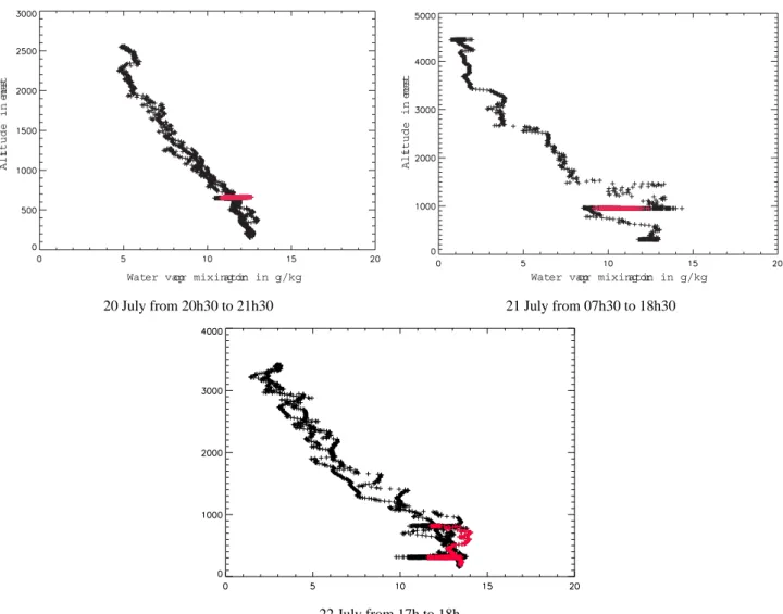
Results of model runs including photochemistry plus dry de-position are shown in Fig. 6 (orange lines). Dry deposi-tion is simulated in the model when the plume is in the BL, i.e. about 15% of the time. The BL definition in the model is climatologically defined, and so, not specifically calculated for the days of the study. The modelled BL heights for the Lagrangian matches were checked by plotting vertical pro-files of water vapour observed by the P3 aircraft around the Lagrangian matches. The profiles in Fig. 7 show that every time the aircraft was over ocean (profiles a and part of profile b), the BL height was less than 0.4 km and so the plume was above the BL, whereas over land, the BL height was between 1 and 1.5 km and the plume was in the BL. This corresponds
ppbv pptv ppbv ppbv ppbv pptv
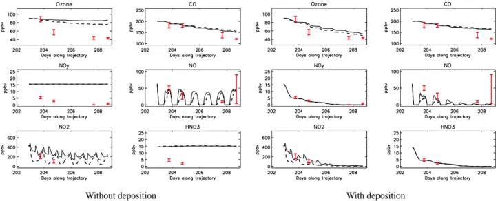
Fig. 6. Modelled concentrations versus time (Julian days) without
deposition (black lines), with dry deposition only (orange lines), with WET1 wet deposition+dry deposition (pink lines), with WET2 wet deposition +dry deposition (bllue lines), and with S-WET3 wet deposition+dry deposition (green lines). Precipitation interpolated from ECMWF precipitation rates (sum over total col-umn) are also shown in lower left panel.
well to the model simulation which has no dry deposition during the 2 first Lagrangian samplings over sea on 20 and 21 July and dry deposition active on 22 July when the trajec-tory passed over land. Inclusion of dry deposition in the sim-ulations leads to decreases of 8 and 20% in O3and HNO3,
respectively. However, it is clear that dry deposition alone cannot explain the observed decrease in either HNO3or O3
in this plume. For a plume travelling at lower altitude and spending more time in the BL, a much more important im-pact of dry deposition could be expected. The results are also sensitive to the definition of the BL height and to positional errors in the trajectories as already discussed in Sect. 2. 4.2.2 Wet deposition
As noted already, satellite images and the strong decrease of HNO3 levels in the plume suggest that wet deposition was
active during the transport of this plume away from source regions. In the basic model, wet deposition is parametrised using a local constant loss rate, r (s-1) (run S-WET1). In this study, two new schemes were implemented linking wet depo-sition to more realistic column integrated precipitation rates,
p(mm s−1) taken from ECMWF analyses. The first scheme (S-WET2) is based on Walton et al. (1988) who introduced a wet deposition coefficient, S, such that r=S×p. For a very soluble gas, such as HNO3, Penner et al. (1991) suggested
Alt
itude in met
ers
Water vapor mixing ration in g/kg
Alt
itude in met
ers
Water vapor mixing ration in g/kg
20 July from 20h30 to 21h30 21 July from 07h30 to 18h30
22 July from 17h to 18h
Fig. 7. Vertical water vapour profiles measured by the P3 close to the Lagrangian matches on 20, 21 and 22 July 2004. Measurements made
in the Lagrangian matches are coloured in red.
and 4.7 mm−1 for convective precipitation. The second scheme (S-WET3) uses a classical formula for the simulation of wet loss of a very soluble specie, r=p/L were L represents the quantity of condensed water integrated over the tropo-spheric column (mm). Wentz and Spencer (1998) estimated a value of L from a satellite study using 0.18×(1+(H p)0.5), where H is the rain column depth, taken as equal to 3 km at mid latitudes. In this formulation there is no distinction between convective and stratiform precipitation. These two formulations apply to very soluble gases like HNO3. To
eval-uate r for other trace species (NO3, N2O5, HO2NO2, HO2,
H2O2, HCHO, C2H5OO, C2H5OOH, HONO) in the model,
results from Crutzen and Lawrence (2000) have been used. They determined a factor αspec that varies from 0 for
insol-uble gases to 1 for very solinsol-uble gases, and depends on the Henry’s Law coefficient (see Table 2) in such way that the new local loss frequency, r∗=r×αspec is calculated. Note
that none of these wet deposition schemes makes a
distinc-tion between precipitadistinc-tion within and below clouds since this information was not available from ECMWF for this study.
Results from the runs including dry and wet deposition, S-WET1 (pink lines), S-WET2 (blue lines) and S-WET3 (green lines) are shown in Fig. 6 together with precipitation rates simulated by ECMWF along the trajectory. It can be noted that the Lagrangian matches correspond to periods with very low precipitation which is coherent with the fact that mod-elled photolysis rates agree well with the measurements in runs with no clouds.
In order to compare the rate of decrease of HNO3, a
pa-rameter τ1/2 can be defined as τ1/2=log(2)×rmean1 where
rmeanis the mean local loss frequency calculated along the
trajectory. This parameter is the half-life of a trace gas cor-responding to an exponential decrease in its concentration. It is equal to 19, 15 and 6 h, respectively, for simulations dry +S-WET1, dry +S-WET2 and dry +S-WET3. Results from the run dry +S-WET3 underestimates HNO3concentrations
Table 2. αspecvalues (coefficient factor apply to the wet loss frequency to take into account solubility of species) as a function of effective
Henry’s Law coefficient (Hf ) (see text).
Hf Hf <103 103<Hf <104 104<Hf <105 105<Hf <106 106<Hf <108 Hf >108
αspec 0 0.15 0.5 0.85 0.95 1
by about 2.5 ppbv compared to the measurements on 21 July. Results from the dry +S-WET1 and dry +S-WET2 simula-tions compare better with the data even if HNO3 is
under-estimated in the dry +S-WET2 run by about 1.5 ppbv on 21 July, and overestimated in the dry +S-WET1 run by the same order of magnitude.
Overall, results using ECMWF precipitation rates (S-WET2 or S-WET3) do not give better results than S-WET1 even if these schemes are more realistic. Here, and in the following sections, results using wet deposition scheme, S-WET2, have been used because it gives better agreement with HNO3measurements than S-WET3, and is more
physi-cally realistic that S-WET1. Since NOyis mainly made up of
HNO3, the half-life of HNO3with the S-WET2 scheme can
be compared with the one estimated by Stohl et al. (2002) for NOy during the 1997 North Atlantic Regional Experiment
(NARE) also off the north-east coast of North America. In that study τ1/2was estimated to be around 40 h, a factor of
2 slower than in the case studied here. This can be partly explained by the fact that air masses selected by Stohl et al. (2002) were rapidly exported out of the BL by frontal warm conveyor belts, and so only subject to wet deposition. The plume studied here stayed in the BL during the first few days, and was therefore influenced by both wet and dry deposition. Overall results from the chemistry and dry/wet deposition runs are closer to the measurements than the chemistry only run. The impact of wet deposition is not only important for HNO3but also for species that are insoluble but dependent on
HNO3 concentrations. Modelled NOxis now almost equal
to zero after 6 days due to lower HNO3photolysis leading to
a reduction in O3production rates which decrease by 60%
due to the impact of wet deposition. This leads to better agreement with the observations, although O3is still
over-estimated by 5 to 10 ppbv on 25 and 26 July and NO under-estimated by 10 to 20 pptv. OH is reduced by 27% when wet deposition is included leading to a slight increase in CO life-time from 20 to 23 days. CO is still overestimated compared to the data suggesting that dilution and mixing were also im-portant as will be seen in the next section. Not only HNO3is
wet deposited but also soluble species like H2O2or CH2O.
A test simulation has been conducted where only HNO3was
wet deposited. Results are similar to those where all solu-ble species are deposited with less than 2% differences. This confirms that the simulated changes when wet deposition is included are almost exclusively due to HNO3removal.
4.2.3 Impact of N2O5hydrolysis
In the runs discussed in the previous sections, heterogeneous loss of trace species on aerosols was not taken into account in the model. This can be important for N2O5 which can
be converted to HNO3through heterogeneous reactions. At
night the conversion of NOx into N2O5becomes the major
NOxsink and if no hydrolysis occurs N2O5decomposes back
into NOxthe following day. However, heterogeneous
reac-tion may be difficult to simulate as there are still some uncer-tainties on the reaction probability value and its dependence on water vapour and temperature. Here, the sensitivity of results to heterogeneous loss of N2O5has been examined
us-ing a parametrisation from Mozurkevich and Calvert (1988). Loss rates were calculated based on recommended tempera-ture and relative humidity dependent uptake coefficient and measurement derived surface aerosol densities using obser-vations made in the plume on 20 July. Since wet deposition and dilution may decrease aerosol density, an exponential de-crease was applied with a half life time of 2 days in order to mimic the decrease in aerosol number between 20 and 21 July. Results of these simulations with and without deposi-tion are represented Fig. 8. When no wet or dry deposideposi-tion is included, the impact of N2O5hydrolysis on NOxand O3
concentrations is important (see Fig. 8a). O3concentrations
decrease by about 5–6 ppbv over 6 days and NOxare lower
by almost 50%. Whilst this leads to better agreement with NOx measurements, HNO3is still overestimated by almost
10 ppbv indicating that loss by wet deposition is a dominat-ing factor in this case. In runs includdominat-ing wet deposition (see Fig. 8b) the impact of including or not including N2O5
hy-drolysis on O3, NO and NO2 levels is less important even
if NOx are significantly reduced with hydrolysis (by about
20%). This is due to the strong deposition of HNO3 and
therefore the strong reduction of NOxin the first couple of
days. Overall N2O5hydrolysis leads to further
underestima-tion of NO and NO2concentrations. In the following
simu-lations, N2O5hydrolysis is not taken into account.
4.3 Role of mixing
4.3.1 Mixing parametrisation
In the previous runs the plume was considered isolated from the background. In the real atmosphere, plumes are subject to stirring by large-scale winds and mixing by processes such as turbulence. Mixing entrains surrounding air masses leading
Without deposition With deposition
Fig. 8. Modelled concentrations versus time (Julian days) for reference runs (continuous lines) and runs including hydrolysis of N2O5
(dashed lines) (a) without deposition (b) with wet and dry deposition.
Table 3. Measured concentrations in the vicinity of the Lagrangian plume used as background concentrations for the mixing simulations
(see text for details).
Time windows CO (ppbv) O3(ppbv) NOy(pptv) NO (pptv) 21 h, 20 July–12 h, 21 July 182 73 6109 120 12 h, 21 July–12 h, 22 July 184 78 4085 55 12 h, 22 July–12 h, 23 July 170 65 3502 42 12 h, 23 July–22 h, 25 July 90 30 150 10 22 h, 25 July–26, July 130 47 5910 1160
to changes in plume concentrations. In the model, mixing is treated as a simple linear relaxation (Evans et al., 2000) with an exponential decay of plume concentrations towards back-ground concentrations using a typical time scale, τ -mix. Due to the Lagrangian aspect of this work, measurements made in the vicinity of the plume during the 5 match segments can be used to estimate background concentrations. This method was already successfully applied to the to the forest fire case discussed in (Real et al., 2007).
Therefore, measurements of NO, O3, CO, C2H4, C2H6,
C2H2, C3H6, C4H10, NOy(for background of the last 3 days)
and PAN, HNO3, C5H12, C6H6, C7H8, methanol,
acetalde-hyde, acetone (for background of the first 3 days) made in plume vicinity were used as background concentrations (see Table 3 for NO, NOy, O3and CO concentrations.
During the first 3 days, the so-called background concen-trations were polluted. Indeed, pollutant concenconcen-trations mea-sured by the P3 on 20, 21 and 22 July between the ground and 2 km were always elevated over the Gulf of Maine and Nova Scotia. Measurements of PAN, HNO3, C5H12, C6H6, C7H8,
methanol, acetaldehyde, acetone as well as NO, NOy, O3and
CO observation in the plume vicinity were used to constrain
background concentrations during the first 3 days (see Ta-ble 3). Between 22 and 25 July, the plume left the North American east coast and travelled over the ocean when it can be considered that the plume was no longer surrounded by polluted air masses but by marine air masses. For this reason, air masses typical of marine air, measured in proximity to the plume on 25 July, were used to characterise background air masses from 23 to 25 July. Finally, high concentrations of NO (up to 1.5 ppbv) and NOy(up to 6 ppbv) were measured
on 26 July just after the sampling of the plume. These val-ues were used to define background valval-ues. These NOyrich
air masses were relatively poor in CO and O3but rich in NO
suggesting that they could be due to local ship emissions in the English Channel (Corbett and Koehler, 2003). However, back trajectories also show transport from southern England suggesting a possible urban source.
With regard to the determination of τ -mix, changes in CO are often used since it is usually considered as a good tracer of air mass transport over time periods of several days. How-ever, in this case, the decrease in CO is strongly influenced by photochemical processes, and is not a very good indicator of dilution and mixing. Arnold et al. (2006) evaluated a τ of 10
days, with a method based on hydrocarbon ratio changes, for plumes crossing the North Atlantic during the ICARTT cam-paign. The same τ was used here except for the last day when a faster mixing rate was used (τ =2 days) when plume entered the European BL in order to represent the strong increase in NO and NOyobserved on 26 July. It should be noted that
CO and O3concentrations measured on 26 July in the
vicin-ity of the plume are very close to the levels in the plume itself and so the plume was not easily distinguishable from the background based on these measurements alone. The mixing time-scale of 10 days, used during the first 5 days, implies slightly weaker mixing rates compared to previous studies (Real et al., 2007; Price et al., 2004). This could be related to the plume remaining relatively intact during trans-port due to strongly converging low level winds, and the fact that the plume was decoupled from the marine BL during transport making mixing and dilution less important in this case. However, the impact of the choice of mixing rate is also dependent on the choice of background concentrations dur-ing transport. For example, applydur-ing a stronger mixdur-ing rate during the first 3 days would only change the results slightly because the background concentrations are not very different from those in the plume and the entire Nova Scotia/Gulf of Maine region was influenced by pollution during this period. The choice of mixing rates is case specific and cannot neces-sarily be taken as representative of mixing rates in the lower troposphere.
4.3.2 Results: chemistry, deposition and mixing
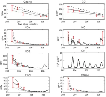
Model results including chemistry, deposition and mixing processes are shown in Fig. 9. During the first 5 days, mixing does not change concentrations very much, mainly because of the low mixing rate used, and the fact that background concentrations used during the first 3 days are not very dif-ferent from those in the plume. Overall, there is now good agreement between the model results and the measurements for the entire period except for 22 July further supporting the hypothesis that this match is not truly Lagrangian. The agree-ment on with the data on 21 July is generally good although NO is still underestimated by about 20 pptv. There is good agreement with CO and O3data in the Lagrangian match on
25 July, with further decreases of 13 and 6 ppbv compared to the runs without mixing, respectively, but NO is still underes-timated. However, observed NO is very low by this time and close to the detection limit of the instrument. Modelled con-centrations are also closer to the data on 26 July, especially for NO which is mixed with higher background concentra-tions. These differences are analysed further in the following section using O3/CO and NOy/CO correlations.
Concerning modelled OH values, the runs including de-position and mixing lead to a reduction in OH of 25% with an average value of 3×10⁶molecs. cm−3over the pe-riod from the 21 to 25 July, with peak noon values of 14×106molecs. cm−3. These values are still slightly higher
pptv pptv ppbv ppbv pptv ppbv ppbv
Fig. 9. Modelled concentrations versus time (Julian days) for
runs including chemical, deposition and mixing processes using mean±std concentrations (same as Fig. 4).
than measurements from George et al. (1999) in recent pol-luted plumes and in better agreement with Ehhalt and Roher (2000). Moreover, since modelled J-values and O3agree well
with the data we can have some confidence in OH results. It is also interesting to re-examine the comparison with measured VOCs. Whereas all VOCs measured on 25 July were underestimated in the run with chemistry only, the model results including deposition and mixing for the long lived VOCs are now in better agreement with the data mainly because of the decrease in modelled OH. For example, on 25 July, the comparisons are 1076 pptv, 159 pptv and 22 pptv for modelled C2H6, C2H2and C4H10compared to measured
val-ues of 1075 pptv, 169 pptv and 25 pptv, respectively. On the other hand, modelled C2H4and C3H6, with shorter lifetimes
of 2 and 0.8 days, respectively, are almost zero whereas the data in the Lagrangian match shows values around 100 pptv for both gases. Since it is unlikely that a plume older than 5 days would have such high concentrations it is possible that the plume was mixed with air masses influenced by local oceanic or biogenic emissions off the coast of Ireland (Heard et al., 2006). Such air masses with elevated levels of alkenes and low CO and O3were measured off the Ireland coast on
the same day by the Falcon.
4.3.3 Influence of the different processes on plume concen-trations
By analysing simulated O3production and destruction terms,
the influence of chemical, deposition and mixing processes on O3can be evaluated. In the runs including all processes,
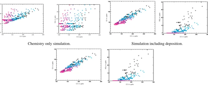
CO in ppbv O3 in ppb v 100 150 50 0 100 150 200 250 300 NO y in ppb v 0 10 20 40 CO in ppbv 100 150 200 250 300 30 O3 in ppb v CO in ppbv NO y in ppb v CO in ppbv
Chemistry only simulation. Simulation including deposition.
O3 in ppb v CO in ppbv NO y in ppb v CO in ppbv
Simulation including deposition and mixing.
Fig. 10. Simulated concentrations of O3and NOyversus CO in the 5 Lagrangian samplings. Black crosses represent measurements during
the 20 July Lagrangian match and green triangles, blue diamonds, pink squares and violet stars show the modelled concentrations during the 21, 22, 25 and 26 Lagrangian samplings, respectively.
Table 4. Measured and simulated O3/CO and NOy/CO correlation slopes with and without mixing and deposition during P3 matches on 20,
21 and 22 July and Falcon matches on 25 and 26 July. Measured correlation coefficients, r, are also reported in brackets.
Measured Simulated without mixing Simulated with deposition Simulated with deposition
slopes or deposition (Case a) (Case b) and mixing (Case c)
P3–20:O3/CO 0.47 (0.91) :NOy/CO 0.31 (0.85) P3–21:O3/CO 0.51 (0.93) 0.52 0.46 0.46 :NOy/CO 0.09 (0.85) 0.27 0.09 0.09 P3–22:O3/CO 0.17 (0.21) 0.59 0.45 0.45 :NOy/CO 0.02 (0.3) 0.29 0.05 0.05
Falcon 25:O3/CO −0.03 (−0.12) 0.69 0.36 0.37
:NOy/CO 0.001 (0.32) 0.3 0.0015 0.0015
Falcon 26 :O3/CO −0.31 (−0.35) 0.66 0.33 0.33
:NOy/CO 0.14 (0.7) 0.27 0.0011 0.0011
42 ppbv in O3concentrations over 6 days is calculated. Of
this decrease 75% is due to chemical destruction, including the effects of dry and wet deposition on O3production, which
gives a mean net O3production of −5 ppbv/day. The
remain-ing 25% is due to direct O3dry deposition (10%) and mixing
(15%). Without wet and dry deposition the net O3production
is only −1.1 ppbv/day. This is mainly due to HNO3
photoly-sis providing a source of NOxas discussed previously. Thus,
these model results show that deposition processes were in-directly responsible for 80% of the impact of photochemistry on O3, with the large majority (78%) being due to wet
depo-sition rather than dry depodepo-sition. Modelled CO decreases by 60 ppbv which is in good agreement with the observed
evo-lution in the plume. Analysis of model results shows that 66% is due to chemical destruction and 34% due to mixing and dilution of the plume. Therefore, in this case, photo-chemical processes governed the evolution of both O3 and
CO in the plume. Whilst this has been shown previously to be the case for O3, this is the first time, to our knowledge,
that photochemistry has been shown to be the dominant pro-cess governing CO evolution over a period of several days. If the plume had not been subject to deposition processes, it would have reached Europe with much higher O3 (80–
90 ppbv), and lower CO (120–140 ppbv). It can be envis-aged that less polluted plumes originating from North Amer-ica would reach Europe with even lower CO values due to
strong OH oxidation, and may therefore not be detected us-ing the methods often applied to diagnose pollutant plumes such as the application of CO thresholds (Li et al., 2002). This point is discussed further in the next section.
4.4 Trace gas correlations
Comparison of the full range of observed and simulated con-centrations in the Lagrangian match samplings, and their inter-relationships can provide useful additional information about the evolution of pollutant concentrations in a plume, than just comparing modelled and measured means ±std along a trajectory. Observed correlations in the Lagrangian matches have already been discussed in Sect. 2. In this sec-tion, multiple runs are used in order to characterise the vari-ability across the Lagrangian samplings in an attempt to re-produce and understand the observed changes using the cor-relation between trace species. This method has already been used successfully to the forest fire case sampled during ICARTT (Real et al., 2007).
Multiple model runs were initialised with P3 measure-ments averaged every 30s during 20 July Lagrangian match samplings. With this method, each run represents a differ-ent part of the initial correlation (black crosses in Fig. 10) observed by the P3. Model results (O3/CO and NOy/CO)
af-ter 1 (green triangles), 2 (blue diamonds), 4 (pink squares) and 5 (violet stars) days are shown in Fig. 10 for 3 cases : chemistry-only simulations (case A), simulations with chem-istry and wet plus dry deposition (case B), and simulations with chemistry, deposition and mixing (case C). The simu-lated slopes for the different cases are reported in Table 4.
It has already been seen in Sect. 4.1 that the chemistry-only runs were unable to reproduce the chemical evolution of the plume but, nevertheless, it is still interesting to exam-ine the evolution of the slopes in the case without deposition or mixing. The O3/CO and NOy/CO simulated in case A
are very different from those observed. The slopes increase with time whereas the data show an overall decrease. The modelled increase is not due to an increase in NOy or O3
that remains nearly constant, but is due to the strong chem-ical destruction of CO in these runs. Therefore, in the run with chemistry only, an increase in the O3/CO slope is the
result of a decrease in CO, and not the result of photochem-ical O3 production as is often stated (Andreae et al., 1994;
Mauzerall et al., 1998). Along the same lines, Chin et al. (1994) showed that a decrease in O3/CO slopes could be due
to the secondary production of CO by hydrocarbon oxidation in a fresh plume, and not just due to chemical destruction or deposition of O3. When deposition processes are included
(case B), NOy/CO slopes show very good agreement with
those observed on 21 and 25 July but not on 26 July. Mod-elled O3/CO slopes now decrease but less than observed on
25 July. Because mixing is simulated as a homogeneous pro-cess, modelled slopes change little between cases B and C due to small changes in O3production. However, the
corre-O3 in ppb
v
CO in ppbv
Fig. 11. Measured O3versus CO concentrations during the 25 July
Lagrangian match from 15:54 to 16:09 (blue crosses, part 1) and from 16:09 to 16:21 (black crosses, part 2). See text for discussion.
lation lines are shifted towards “background” concentrations, and the dispersion is reduced (see also discussion in Real et al., 2007). This leads to better overall agreement with the data in this correlation space although there are still some differences. The bad match between measurements and sim-ulations on the 22 July has already been identified using the analysis based on comparison with mean observed values in the Lagrangian matches (Sect. 4.1) and is not discussed fur-ther.
Interestingly, this approach shows differences in measured and modelled O3/CO slopes (−0.03 and 0.36, respectively)
on 25 July that were not apparent in the analysis using mean concentrations when model results agreed well with data. Further analysis based on the correlations suggests that the measurements in this Lagrangian match can be divided into 2 different parts, from 15:54 to 16:06 and 16:06 to 16:21, and 2 different air masses may have in fact been sampled. This distinction is shown in Fig. 11 based on the observed O3/CO correlation. For the first segment, CO and O3are not
really correlated, with a slope of 0.02 whereas for the sec-ond segment, the slope is positive with a value of 0.28, and a correlation coefficient of 0.75. This slope is comparable to measured values at ground-based sites such as Mace Head (Li et al., 2002). It is also closer to the simulated slope (0.36) whereas the weak slope in the first segment is not reproduced by the model runs initialised with measurements on 20 July. Therefore, it seems that the second segment represents the best match with the plume from 20 July whereas the first segment appears to have been influenced by inhomogeneous mixing at the edges of the plume, possibly with marine air masses, and not reproduced by the model.
The last important difference between modelled and mea-sured NOy/CO slopes is seen in the evolution between the
25 and 26 July. The observed slopes are particularly much steeper on 26 July compared to 25 July. The Lagrangian plume appears to have been strongly dispersed by the time it it reached the English Channel on 26 July and influenced by fresh emissions with very high levels of NO and NOy,
as noted previously. The model does not capture this vari-ability since the plume is not mixed with the full range of concentrations in this local plume but only with mean con-centrations. Therefore, this last sampling cannot be consid-ered as Lagrangian because of the strong influence of recent emissions.
5 Conclusions
The case of an anthropogenic plume transported from North America (New York-Boston region) over the North Atlantic to Europe at low altitudes has been studied in a Lagrangian framework. This plume was initially strongly polluted with high concentrations of O3, CO and NOx, typical of North
American polluted plumes, and also very high levels of HNO3. During transport, all pollutant concentrations
de-creased, and the plume was much less polluted when it was intercepted off the west coast of Ireland several days later. A Lagrangian photochemical model (CiTTyCAT), has been used to assess the different processes influencing the evolu-tion of pollutant levels in the plume during long-range trans-port. Average concentrations and correlations between trace species (O3/CO and NOy/CO) have been examined and
com-pared to data collected in the Lagrangian match segments. Overall, the analysis suggests that some of the links identi-fied as Lagrangian by Methven et al. (2006) are not truly La-grangian, in particular on 22 July because of probable errors in ECMWF coastal winds and on 26 July due to the influ-ence of local emissions. In addition, the analysis of trace gas correlations showed that part of the match on 25 July is not closely linked to 20 July.
The evolution of the chemical composition in the plume (mean values and correlations) is best reproduced when pho-tochemistry, dry/wet deposition and mixing with surround-ing air masses are all included. Model results show that these changes were mainly driven by photochemical and de-position processes, especially wet dede-position. The impact of heterogeneous loss of N2O5on aerosols can be important
for NOx(50% reduction) and O3but much less in this case
where wet deposition is the dominant factor affecting NOy.
Mixing with air masses in close proximity to the plume dur-ing transport did not have a strong impact on trace gas con-centrations during the first 5 days due to strong and rapid transport by low level winds and isolation of the plume from the marine boundary layer over the Atlantic. Mixing with local pollution sources (possibly ships or urban sources) ap-pears to have been important on 26 July.
Mean net O3 production in the plume was negative over
the 6 day period averaging about −5.0 ppbv/day leading to
average O3 concentrations of 44 ppbv when it reached
Eu-rope. This is low compared to values observed close to Euro-pean sources but is significantly higher than levels observed over remote oceanic regions where the plume was sampled and so may represent a net import affecting background O3
levels over western Europe. Plume O3was directly impacted
by dry deposition, and indirectly by wet deposition through the strong scavenging of HNO3, mainly in the first couple of
days of transport. This implies that, in this case, wet deposi-tion was responsible for an 80% reducdeposi-tion in net photochemi-cal O3production. This study and the one from Neuman et al.
(2006) show that, because polluted plumes from the New-York/Boston region are very rich in HNO3, wet deposition
can have a strong impact on O3levels downwind. Runs with
no wet deposition, showed that photolysis of HNO3 could
maintain high O3 during plume transport leading to lower
average net destruction (−1.0 ppbv/day). In that case, the plume would have reached Europe with O3 concentrations
between 80 and 90 ppbv resulting in a stronger import of O3
directly into the European BL.
Another important result is the dominant influence of pho-tochemistry on CO concentrations in the plume rather than mixing and dilution which is usually assumed to be dominat-ing over these time scales. In this case, photochemical de-struction explains 66% of the CO decrease compared to only 34% due to mixing. This is due to relatively high O3
lev-els during the first few days coupled with high water vapour leading to a high oxidative capacity in the plume, and there-fore a reduction in CO chemical lifetime to 23 days. This has several consequences. Firstly, these results show that, in this case of pollutant transport at low altitudes, CO can-not be always used as a tracer of anthropogenic pollution. This may also explain the low levels of CO often observed in plumes originating from North America and sampled down-wind in the European BL. The latter does not imply that the plume was weakly polluted but that photochemistry was in-tense. Secondly, we have shown that an observed increase in O3/CO correlation slopes can result from photochemical
destruction of CO and not photochemical production of O3
as is often assumed.
Overall, these results show that O3import into downwind
regions is sensitive to scavenging processes along route as well as photochemical processing and that CO levels can also be strongly influenced by photochemical loss as well as dilu-tion and mixing. Whilst there are uncertainties related to this type of Lagrangian analysis including errors in trajectories, studies using this modelling framework are able to provide detailed insight into the processes governing pollutant plume evolution during long-range transport. These results can also be used to evaluate plume transport and processing in global models that typically have problems resolving such features. Acknowledgements. Elsa Real and Kathy Law acknowledge financial support from national programmes (PNCA, PATOM) provided by INSU-CNRS, ADEME and also from Insitut Pierre