Evaluation of the MERIS aerosol product over land with AERONET

(1)

HAL Id: hal-00328311

https://hal.archives-ouvertes.fr/hal-00328311

Submitted on 10 Oct 2008

HAL is a multi-disciplinary open access

archive for the deposit and dissemination of sci-entific research documents, whether they are pub-lished or not. The documents may come from teaching and research institutions in France or abroad, or from public or private research centers.

L’archive ouverte pluridisciplinaire HAL, est destinée au dépôt et à la diffusion de documents scientifiques de niveau recherche, publiés ou non, émanant des établissements d’enseignement et de recherche français ou étrangers, des laboratoires publics ou privés.

Evaluation of the MERIS aerosol product over land with

AERONET

J. Vidot, R. Santer, O. Aznay

To cite this version:

J. Vidot, R. Santer, O. Aznay. Evaluation of the MERIS aerosol product over land with AERONET. Atmospheric Chemistry and Physics Discussions, European Geosciences Union, 2008, 8 (1), pp.3721-3759. �hal-00328311�

(2)

ACPD

8, 3721–3759, 2008

MERIS aerosol product over land

J. Vidot et al. Title Page Abstract Introduction Conclusions References Tables Figures ◭ ◮ ◭ ◮ Back Close

Full Screen / Esc

Printer-friendly Version Interactive Discussion

EGU

Atmos. Chem. Phys. Discuss., 8, 3721–3759, 2008 www.atmos-chem-phys-discuss.net/8/3721/2008/ © Author(s) 2008. This work is licensed

under a Creative Commons License.

Atmospheric Chemistry and Physics Discussions

Evaluation of the MERIS aerosol product

over land with AERONET

J. Vidot1, *, R. Santer2, and O. Aznay2

1

Atmospheric and Oceanic Sciences Department, University of Wisconsin, Madison, USA

2

Laboratoire Interdisciplinaire des Sciences de l’Environnement, Maison de la Recherche en Environnement Naturel, Universit ´e du Littoral Cote d’Opale, Wimereux, France

*

now at: Lab. de M ét éorologie Physique, Universit é Blaise Pascal, Clermont-Ferrand, France Received: 12 October 2007 – Accepted: 23 January 2008 – Published: 25 February 2008 Correspondence to: J. Vidot (j.vidot@opgc.univ-bpclermont.fr)

(3)

ACPD

8, 3721–3759, 2008

Full Screen / Esc

EGU

Abstract

The Medium Resolution Imaging Spectrometer (MERIS) launched in February 2002 on-board the ENVISAT spacecraft is making global observations of top-of-atmosphere (TOA) radiances. Aerosol optical properties are retrieved over land using Look-Up Table (LUT) based algorithm and surface reflectances in the blue and the red spectral

5

regions. We compared instantaneous aerosol optical thicknesses retrieved by MERIS in the blue and the red at locations containing sites within the Aerosol Robotic Network (AERONET). Between 2002 and 2005, a set of 500 MERIS images were used in this study. The result shows that, over land, MERIS aerosol optical thicknesses are well retrieved in the blue and poorly retrieved in the red, leading to an underestimation

10

of the Angstrom coefficient. Correlations are improved by applying a simple criterion to avoid scenes probably contaminated by thin clouds. To investigate the weakness of the MERIS algorithm, ground-based radiometer measurements have been used in order to retrieve new aerosol models, based on their Inherent Optical Properties (IOP). These new aerosol models slightly improve the correlation, but the main problem of the

15

MERIS aerosol product over land can be attributed to the surface reflectance model in the red.

1 Introduction

There is a clearly need for an accurate representation of the distribution of aerosols over the globe not only because of their direct and indirect radiative impacts on

cli-20

mate (IPCC, 2007), but also because of their health impact on population (Wilson and Sprengler, 1996). The representation of the aerosols optical properties distribution is provided by several tools, from satellite aerosols products (Kaufman et al., 2002), sur-face measurements (Dubovik et al., 2002) and aerosol transport model (Chin et al., 2002). Information about aerosol absorption is often needed for radiative impact

pur-25

(4)

ACPD

8, 3721–3759, 2008

Full Screen / Esc

EGU

space sensors (Mishchenko et al., 2004). From space, actual retrievals on aerosol op-tical properties are mainly based on three different techniques: (i) from multi-bands unpolarized measurements, (ii) with polarization and/or (iii) multidirectionnality. All of these different techniques provide advantages/inconveniences on the aerosol retrieval. For example, multi-bands unpolarized sensors like the Moderate Resolution Imaging

5

Spectroradiometer (MODIS) sensor allow a good spatial resolution at the ground but can provide information on total column amount and size of aerosols (Remer et al., 2005). The aerosol parameters have been recently improved with the MODIS Second Generation Algorithm (Levy et al., 2007) and the “Deep-Blue” algorithm (Hsu et al., 2006). These new algorithms enhanced the possibility to discriminate dust particles

10

from fine aerosols. Using the multidirectionnality as the Multiangle Imaging Spectrora-diometer (MISR) sensor, provide constraints on the surface reflectance and on scatter-ing properties of aerosols (Abdou et al., 2005). Addscatter-ing the polarized measurements like POLDER increases the information content and provides constraints on the surface reflectance and on the fine mode of the aerosol distribution (Deuz ´e et al., 2001).

15

The Medium Resolution Imaging Spectrometer (MERIS) instrument can also assume an integral role in the effort of obtaining a global picture of aerosols due to its frequent global measurements of aerosol amount and type over a wide variety of surface types. The primary goal of MERIS is the ocean color observation, while the secondary pur-pose is the observation of the atmosphere and the terrestrial surface. MERIS is one

20

of the instruments of the ENVISAT satellite launched in 2002. ENVISAT is a sun-synchronous orbit with an equator crossing time of 10 a.m. local time. MERIS is a pro-grammable, medium-spectral resolution, imaging spectrometer operating in the solar reflective spectral range. Fifteen spectral bands can be selected by ground command, each of which has a programmable width and a programmable location in the 390 nm

25

to 1040 nm spectral range. The instrument’s 68.5◦ _{field of view around nadir covers a} swath width of 1150 km with a resolution of 1200 m at the ground (Rast et al., 1999). The MERIS accuracy is ±4% in reflectance (Delwart et al., 2003). The absolute un-certainties of the vicarious calibration of MERIS over land are found between 3 and

(5)

ACPD

8, 3721–3759, 2008

Full Screen / Esc

EGU

7%, depending on the accuracies of the available ground truth data (Kneubuehler et al., 2004).

In this article, we evaluate the MERIS aerosol product over land. The first part will be devoted to the presentation of the general aspects of the aerosol retrieval over land from multi-channel sensors working in visible (VIS) to near infrared (NIR)

spec-5

tral regions. Both 1st and 2nd MERIS processing are described. The second part presents the world-wide ground-based aerosol measurement Aerosol Robotic Network (AERONET) sites that we used in the evaluation of the MERIS aerosol product over land. The third section will compare the MERIS aerosol product over land against AERONET outputs, then describes a new aerosol models family based on AERONET

10

sky radiances measurements. The new aerosol model family obtains Inherent Optical Properties of aerosols (IOPA) that slightly improved the MERIS aerosol product over land. Lastly, we will point out the weakness of the surface reflectance that explains the poor MERIS aerosol product over land in the red.

2 MERIS aerosol retrieval

15

2.1 Generality of the MERIS aerosol remote sensing over land

Aerosol remote sensing over land from space is a very difficult task because of the high reflectivity of the Earth compared to the aerosol scattering signal in the back-scattering region. The technique chosen for MERIS (Santer et al., 1999) relies on the well known Dense Dark Vegetation (DDV; Kaufman and Sendra, 1988) concept,

20

generalized to the dark target concept of MODIS (Kaufman et al., 1997). The idea here is to detect dark and stable targets whose reflectivity is know accurately with a simple and reliable method. For MERIS, the Atmospherically Resistant Vegetation Index (ARVI; Kaufman and Tanr ´e, 1992) was used to detect DDV pixels, whereas the MODIS team uses the capability to observe in the near infrared at 2.1 µm for detecting

25

(6)

ACPD

8, 3721–3759, 2008

Full Screen / Esc

EGU

accuracy of the reflectance model of the target and the aerosol models, which were used for the computation of the aerosol scattering functions.

2.2 The aerosol retrieval in the 1st MERIS processing

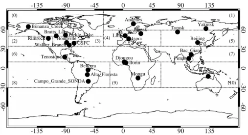
In the case of MERIS, 11 biomes have been chosen to represent the spatial and the temporal variations of the DDV concept over the globe. Figure 1 gives the

geograph-5

ical distribution of the 11 biomes (represented by dashed boxes with the number in brackets, from 0 to 10). Table 1 provides the model name of each biome. For each biome a set of Look Up Tables (LUT) has been generated that gives the DDV Bidirec-tional Reflectance Function (BRDF) in the blue (at 443 nm) and the red (at 670 nm) and the coupling terms between the DDV and the atmosphere (Ramon and Santer,

10

2001). The aerosol characterization is based on aerosol models. They are defined by a size distribution n(R) of particles of radius R represented by the Junge power law, n_(R)≈R−(α+3)_{, and by 26 values of the Angstrom coefficient α (from 0 to 2.5 by step of} 0.1). These models will be called Junge models hereafter. They are also defined by 3 values for the real part of the refractive index m (1.33, 1.44 and 1.55). No absorption

15

has been included in the aerosol models. At the present time, the aerosol refractive index is set to 1.44 by default, which corresponds to a standard continental aerosol model. The aerosol optical properties (extinction coefficient, single scattering albedo and phase function) have been precalculated at 550 nm with the Mie theory. Aerosol optical thicknesses (AOTs) τain the red and in the blue are retrieved for each Angstrom

20

coefficient α. The model for which the Angstrom coefficient is the closest to the one that is obtained from the τ_a retrieval is the model that we select. The aerosol product of the 1st MERIS processing consists of τaat 865 nm and α.

2.3 The aerosol retrieval in the 2nd MERIS processing

Because the concept of DDV was too restrictive in order to get a good spatial

repre-25

(7)

ACPD

8, 3721–3759, 2008

Full Screen / Esc

EGU

brighter surfaces called Land Aerosol Remote Sensing (LARS; Santer et al., 2007a). The LARS surface reflectance has a linear dependence with the ARVI. The aerosol product offers a much better spatial coverage but also introduces more errors in the τa

and α retrievals. These errors occur mostly in the red, as the variation of the surface reflectance with the ARVI is more pronounced than in the blue and therefore most

sub-5

ject to uncertainties. Preliminary tests of the aerosol retrieval using the LARS indicated a large and random spatial distribution of α rending suspect the retrieval of τ_a in the red. Efforts were made to improve the characterization of the surface reflectance in the blue and in the red using the MODIS level 3 albedo maps (Moody et al., 2003) to produce the required surface reflectance. Both the offset and slope of the linear

depen-10

dence with the ARVI, in a 1◦_{by 1}◦_{spatial grid, have been defined (Ramon and Santer,} 2005). The initial 11 biomes are kept in order to describe the BRDF of the LARS pixels. Nevertheless, α values were still suspicious. They are flagged because out of range values (0–2.5) on numerous occasions. Therefore, the following decisions were taken: (i) to output τa at 443 nm instead of τa at 865 nm because of the disastrous effect of

15

α, ii) to produce the τain the blue using the Junge model of α=1 and (iii) to output α

as an indicator of the aerosol type as it was computed for the 1st processing. Then, the aerosol product of the 2nd MERIS processing consists of τain the blue (at 443 nm)

and α.

3 AERONET data

20

AERONET is a globally distributed network of automated ground-based instruments and data archive system, developed to support the aerosol community. The instru-ments used are CIMEL spectral radiometers that measure the spectral extinction of the direct Sun radiance (Holben et al., 1998). The aerosol optical depths are deter-mined using the Beer-Bouguer Law in several spectral bands. For this study, level-2

25

data are used and consist of τ_aat 440 nm and 675 nm, retrieved at least every 15 min during day time. Level-2 data are cloud-free and quality assured retrieved from

(8)

pre-ACPD

8, 3721–3759, 2008

Full Screen / Esc

EGU

and post-field calibrated measurements (Smirnov et al., 2000). The estimated accu-racy in the AERONET τais between ±0.01 and ±0.02 and depends on the wavelength,

for an airmass equal to 1 (Dubovik et al., 2000).

We selected geographically diverse AERONET sites that provided generally good-quality measurements records between 2002 and 2005. A total of 24 AERONET sites

5

have been selected in order to cover the 11 biomes of MERIS and the range of pos-sible aerosol optical thicknesses from clean areas to turbid ones (due to different air masses types and sources as biomass burning, continental and/or dusty conditions). Figure 1 gives the geographical distribution of AERONET sites (represented by black dots). We optimally selected three AERONET sites per biome. Unfortunately, biomes 2

10

(MidLat West America), biome 6 (Tropical America) and biome 10 (Equatorial Asia) are under represented with only one site because of the lack of AERONET sites, the lack of AERONET measurement or the area not covered by vegetations (mainly desert or snow-covered areas). Information about AERONET sites per biome (name and Princi-pal Investigator of the site) are provided in Table 1. We also gave the range of τain the

15

blue and the range of α over the number of match-ups (N) that have been used in this study.

Biome 0 (Boreal America) is represented by three AERONET sites that cover τa

in the blue from 0.04 to 1.96 and α between 0.6 and 1.9. The large value of α is representative of small particles. The artic atmosphere is generally clear but frequently

20

subjected to forest fires in Alaska. Jet streams also transport pollution from Asia or other source regions into this region (Bokoy ´e et al., 2002). Biome 1 (Boreal Euroasia) is represented by two AERONET sites but suffers from a lack of match-ups (N=11) and low variability of τa in the blue (from 0.07 to 0.31). Those regions can also be

subjected by long range transport of artic haze (Toledano et al., 2006) or forest fires,

25

that explains the high values of the α (up to 2.2). Biome 2 (Mid Latitude West America) is represented by only one AERONET site and few match-ups (N=4) where τain the

blue is between 0.14 and 0.79. This part of North America can be affected by aerosols transported from Eurasia. Biome 3 (Mid Latitude West America) is represented by

(9)

ACPD

8, 3721–3759, 2008

Full Screen / Esc

EGU

three AERONET sites with τ_a in the blue from 0.03 to 1.41. Biome 4 (Mid Latitude Europe) is represented by three AERONET sites with τain the blue from 0.02 to 1.47.

AERONET sites of biomes 3 and 4 are continental sites that cover a diversity of urban and industrial pollution aerosols (Kahn et al., 2005). Biome 5 (Mid Latitude Asia) is represented by two AERONET sites with τa in the blue from 0.09 to 2.96. Due to

5

combined influences of arid dust region production and increased fossil fuel usage, the East Asia regions often experience very high concentrations of tropospheric aerosols (Eck et al., 2005). Biome 6 (Tropical America) is represented by one AERONET site with τain the blue from 0.1 to 2.22. The Mexico area is considered as a heavily urban

polluted site. Biome 7 (Tropical Asia) is represented by two AERONET sites with τ_a in

10

the blue from 0.34 to 1.4. Those different sites are industrialized urban area (Grey et al., 2006). Biome 8 (Equatorial America) is represented by three AERONET sites with τain

the blue from 0.05 to 1.26. The Amazonian Basin is a great source of biomass burning aerosol during the period from August to October (Schafer et al., 2002). Biome 9 (Equatorial Africa) is represented by three AERONET sites with τa in the blue from

15

0.04 to 0.59. Africa is an important source of desert dust and biomass burning aerosols (Eck et al., 2001). Biome 10 (Equatorial Asia) is represented by one AERONET site with τain the blue from 0.08 to 0.24.

The different sites we selected will give us a good picture of the quality of the MERIS aerosol optical depths over land. However, for some biomes, we do not expect to

20

make any conclusion on the quality of the MERIS aerosol retrieval due to the lack of match-ups (such as biomes 2 and 10).

4 The Results

4.1 Initial validation

In order to take into account both the spatial and temporal variability of aerosol

distribu-25

(10)

ACPD

8, 3721–3759, 2008

Full Screen / Esc

EGU

direct Sun measurements need to be collocated in space and time. We required at least 2 out of possible 5 AERONET measurements within ±30 min of MERIS over-passes and at least 10% out of possible MERIS retrievals in a square box of 10×10 pixels centered over AERONET sites (that represent 10 measurements). The mean values of the collocated spatial and temporal ensemble are then used in linear

regres-5

sion and root mean square errors (rmse) analysis. The total number of match-ups we obtained was 500 for the 24 AERONET sites between 2002 and 2005. The left panel of Table 2 give an overview of the results between 2nd processing MERIS and AERONET τain the blue. The number of match-ups N, the correlation coefficient r, the

linear regression equation coefficients (slope and intercept) and the rmse are provided

10

for each biome. For biomes 1 and 10, correlations are poor (with correlation coefficient of 0.23 and 0.37, respectively) certainly due to a wrong surface reflectance model in these extreme areas. The correlation for biome 2 is perfect (r=1) but biased by the few match-ups. For others biomes, correlations are good with at best r=0.93 for biome 0. In most cases, slopes are greater than 1, which implies an underestimation of the

15

MERIS τa compared to the AERONET value. But in some cases, we are very close

to the 1:1 line (for example, see biomes 0 and 4). Intercepts are small and rmse are comprises between 0.139 and 0.53. The latter high value of rmse of 0.53 for biome 5 might be explained by an effect of absorption that is not taken into account in our aerosol models. One particular feature that we can observe in some cases is that

20

MERIS shows a very large value of τa when compared to AERONET. This might be

explained by the presence of thin clouds, like cirrus, that the actual MERIS algorithm is not able to flag. In order to remove these contaminated scenes, we applied a simple threshold on the standard deviation of τain the blue within the box (called σ-filter

here-after). A value of 0.15 seems to be the best value (Ramon, personal communication)

25

in order to remove inhomogeneous scene contaminated by thin clouds. We applied the σ-filter and in the right panel of Table 2, we provided the statistical outputs from the σ-filtered match-ups scatterplots. In most biomes, correlation coefficients slightly increased, rmse decreased without significantly changing neither the slope nor offset

(11)

ACPD

8, 3721–3759, 2008

Full Screen / Esc

EGU

coefficients of the linear regression. However, the σ-filter is not the most efficient test to remove high thin cirrus because (i) they can be very homogeneous over the scene and (ii), they may have an optical thickness lower or near the same order of magnitude as aerosols’. In order to minimize the effect of high, thin cirrus clouds, oxygen pressure can be utilized as an effective mask. Indeed, MERIS offers the possibility to accurately

5

retrieve the cloud top pressure thanks to its window and absorption dual channels in the O2 A-band (Preusker and Fischer, 1999). The use of the cloud top pressure re-trieval is even able to mask very thin cirrus clouds (Ramon et al., 2002). Unfortunately, we did not use the cloud top pressure based mask in our study.

The same comparison has been done in the red. Table 3 provides the summary

10

of statistical outputs from the scatterplots both with and without the σ-filter (i.e., the threshold on the standard deviation of τa in the blue). Main conclusions of the

com-parison are that MERIS overestimates τacompared to AERONET, and the correlations

are reduced in most of the cases in the red than in the blue. In the red, the application of the filter allows us to improve correlations.

15

In order to summarize the comparison, we combine all the data irregardless of their location. Figure 2 indicates the quality of the MERIS retrieval in the blue from the 2nd processing without (Fig. 2a) and with (Fig. 2b) the σ-filter. Correlations in the blue are very good with r=0.8 and a linear regression close to the 1:1 line (slopes of 0.98 and small negative intercept of −0.03). The σ-filter allows to slightly increase the correlation

20

coefficient to 0.83 and to reduce the rmse from 0.215 to 0.2. Figure 3 indicates the quality of the MERIS retrieval in the red from the 2nd processing without (Fig. 3a) and with (Fig. 3b) the σ-filter. Overall, the MERIS τ_a retrieval in the red is not as good as the retrieval in the blue, as r=0.7 (increased to 0.73 with the σ-filter) and with the slope of the regression of 0.57 (increased to 0.62 with the σ-filter). In Figure 4, the similar

25

comparison on α is shown and looks less favorable. In both cases (i.e., for match-ups selected with or without the σ-filter), MERIS shows larger aerosols than AERONET.

(12)

ACPD

8, 3721–3759, 2008

Full Screen / Esc

EGU

4.2 Relevance of the 2nd MERIS processing approach

At this stage, we have only presented the evaluation of the MERIS 2nd processing aerosol product over land. We can alter the Junge models in order to evaluate the 1st processing. Actually, in the 2nd processing, it is partially the 1st processing in the combined retrieval of τa in the blue and in the red (or τa in the blue and α). The main

5

difference is that it is applied to LARS pixels in the 2nd processing, whereas it was applied to DDV pixels in the 1st processing. But α remains unchanged between the two processing on LARS pixels.

In the 1st processing, α was used as the spectral dependence of τ_a in the retrieval of τa in the blue. Then to evaluate the 1st processing, we have to recalculate τa from

10

the 2nd processing aerosol product (i.e., τaand α=1) by using the retrieved α. Fig. 5

gives the results of τ_a in the blue on the σ-filtered match-ups. Taking the retrieved α compared to α=1 leads to a depreciated retrieval of the τain the blue. The correlation

coefficient decreased from 0.83 (2nd processing) to 0.72 (1st processing). The slope also decreased from 1.05 to 0.73, respectively. The rmse increased by 0.071.

15

In order to explain the depreciation, we have to introduce the relation between the aerosol path radiance (La) that MERIS measures and the aerosol product τa. In the

primary scattering approximation, the aerosol path radiance is expressed by:

L0_a₌ τa̟0Pa(θ) 4µv

E_s

π , (1)

where E_s is the solar irradiance for the central wavelength of each spectral band

cor-20

rected for the Sun-Earth distance, ω0is the single scatting albedo, Pathe aerosol phase

function, θ the scattering angle and µv the cosine of the sensor viewing angle.

The depreciated retrievals can now be explained by two effects. First, the product ω₀P_a in the backscattering region (for MERIS θ is comprise between 100◦ _{to 150}◦₎ increases with α. Figure 6 shows ω0Pa versus α for different values of θ. Secondly,

25

(13)

ACPD

8, 3721–3759, 2008

Full Screen / Esc

EGU

overestimates τ_a in the blue. The decision to arbitrary set α=1 for the MERIS 2nd processing is justified.

4.3 Doing better with a new set of aerosol models?

The interpretation of the aerosol path radiance into τa relies on the use of 26 Junge

models. The ability for these aerosol models to describe the aerosol optical properties

5

was reported by Ramon et al. (2003). This validation exercise was based on CIMEL AERONET measurement of the sky radiance in the principal plane. The following methodology, described by Santer and Lemire (2004), was used:

– α between 440 nm and 675 nm is used to select the two boundary Junge models, – The Successive Order of Scattering (SOS; Deuz ´e et al., 1989) code is used to

10

simulate the sky radiance in the principal plane,

– The inputs to the SOS code are the CIMEL τ_a at the time of the sky radiance measurements and with the corresponding geometrical conditions,

– Simulated and measured sky radiances are compared.

This evaluation of the Junge models led to noticeable discrepancies in the sky

radi-15

ance retrieval. A similar approach highlights that the Junge models overestimated the sky radiance with a systematic bias of 10% at 675 nm and 30% at 870 nm (Aznay and Santer, 2007). The performance of the Junge models in the blue is a bit more difficult to conclude because of the predominance of the Rayleigh scattering.

An alternative use of the CIMEL sky radiance is to retrieve ω0Pa(Santer and Martiny,

20

2003; Santer et al., 2007b1). Therefore, the European Space Agency (ESA) undertook an action to produce a new set of aerosol models based on the interpretation of the

1

Santer, R., Zagolski, F., and Aznay, O.: Iterative process to derive aerosol phase function from CIMEL measurements, Int. J. Remote Sens., submitted, 2007b.

(14)

ACPD

8, 3721–3759, 2008

Full Screen / Esc

EGU

CIMEL sky radiances to retrieve the inherent optical properties of aerosols, i.e. the product ω0Pa (called IOPA models hereafter). This new set of aerosol models is still

classified in α for values between 0 and 2.5 by step of 0.1. Results are reported in Zagolski et al. (2007) for a similar approach conducted over water. We shown in Figure 7, the comparison of ω0Pa for different α between the initial values using the Junge

5

models and the IOPA models retrieved from AERONET. The agreement is sometimes excellent, mainly for values of α near 1 (Fig. 7c, d and e).

4.3.1 The MERIS 2nd processing with IOPA models: deriving τain the blue

In the 2nd processing, the α=1 Junge model is selected, so we do not expect to see spectacular changes on the retrieval of τain the blue when replacing the Junge aerosol

10

models by the IOPA models. In order to change the aerosol model, we can at first use the primary scattering approximation to describe the aerosol path radiance (Eq. 1). If we change ω0Pa, then we use a simple ratio technique to derive a new value of τa, that

is given by: τIOPA_a τ_aJunge = (̟0Pa(θ))Junge (̟0Pa(θ))IOPA . (2) 15

But if we modify τ_a, then we have to take into account the change in the multiple scat-tering factor f , defined as the ratio between primary scatscat-tering and multiple scatscat-tering, i.e., L = f L0a= f τ_a̟₀P_a(θ) 4µ_v E_s π (3)

In the MERIS ground segment, the multiple scattering factor f has been implemented

20

in the form of LUT computed with the SOS code and generated for the 26 Junge mod-els. To derive τ_a with the IOPA, we need to reconstruct the aerosol path radiance. It can be done through Eq. (3) with the former Junge models. But the interpretation of

(15)

ACPD

8, 3721–3759, 2008

Full Screen / Esc

EGU

Eq. (3) with IOPA models requires the knowledge of f . It is not so simple to generate a set of new LUTs of f with the IOPA models. We choose, according to some hypothesis, to use f implemented in the MERIS ground segment with the IOPA models. The main hypothesis that we made is that f is the same for two families of aerosol models. To validate this hypothesis, we simulated f with the SOS code for two different families

5

of aerosol models, the Junge models and the Shettle and Fenn (1979) models corre-sponding to the same α. In Fig. 8, we plotted f at 870 nm for three classes of aerosol models (coastal, maritime and rural) with a relative humidity of 50%. The solar zenith angle was set to 70◦ and τa was set to 0.15. As we can see, there is no big difference

between the two families, particularly as to the rural model between 110◦and 150◦of θ.

10

The comparison of the new τ_awith the IOPA models is reported in Fig. 9. The quality of the linear regression is slightly improved; with a slope of 1.01 for IOPA models and 1.05 with the Junge models (Fig. 2b). These changes are not considered to be significant.

4.3.2 The MERIS 1st processing with IOPA model: deriving α and τain the blue

In this part we explored the possibility to return to the 1st processing with the IOPA

15

models. Starting from the aerosol path radiance in the blue, we used theα derived from MERIS and its associated IOPA models that give the ω₀P_a to derive τ_a in the blue. With α, we obtained τ_a in the red. That is the 1st processing and its associated τ_a values. Then, we reconstructed the aerosol path radiance in the red as we did in the blue. We could then vary both aerosol path radiances. So, we used the MERIS

20

algorithm that is described as follows:

1. A double loop is done with 26 αJ (26 Junge models) and with τa to retrieve the

aerosol path radiance. Outputs are 26 values of τa.

2. This double loop is applied in the blue and in the red. The resulting τ_aare reported in Fig. 10.

25

(16)

ACPD

8, 3721–3759, 2008

Full Screen / Esc

EGU

4. When αMERIS=αJ, we get the final τa.

Some comments about Fig. 10 are necessary. When α increases, ω₀P_a increases, as we can see on Fig. 6. Therefore, τa decreases with α in proportion with ω0Pa in

the primary scattering approximation (Eq. 1), and it does a little more when accounting from the multiple scatterings. Because the aerosol phase function has no wavelength

5

dependency, the τa ratio 443/670 is insensitive to α, if we exclude the second order

effect of the multiple scattering. We can now apply the MERIS 1st processing with IOPA models. Figure 11 illustrates the comparison of τ_a in the blue (left panel) and in the red (right panel) with the AERONET outputs. Introducing the IOPA models into the MERIS 1st processing leads to a slight increase of the correlation coefficient in the

10

blue from 0.72 (Junge models) to 0.78 (IOPA) and a decreasing of the rmse from 0.271 to 0.227, respectively. However, the 2nd processing with IOPA gives better results at least in the blue (Table 4). In the red, we still have an overestimation of τacompared to

AERONET.

4.4 Possible errors in the LARS reflectance at 670 nm?

15

With the aerosol models, the other key parameter in the MERIS τa retrieval over land

is the knowledge of the LARS surface reflectance. We expect that an inaccuracy in the LARS surface reflectance has less impact on the τ_aretrieval in the blue when compared to the red for the following reasons: (i) vegetation appears darker in the blue than in the red and (ii) the aerosol signal increases towards the blue. It is clearly the case

20

from the above results (Table 4). To effectively demonstrate this, let us assume that the aerosol type is known. First, let us take α as measured by AERONET. If we have the correct aerosol model with IOPA, then we should have the correct aerosol reflectance if the LARS reflectance is correct. We ran the MERIS 1st processing with the “exact” aerosol type and output the aerosol reflectance. Results are reported in Fig. 12. The

25

retrieval in the blue is a little biased and remains bad in the red, due to the LARS reflectance. In the blue, the MERIS LARS reflectance is a little high, resulting in an

(17)

ACPD

8, 3721–3759, 2008

Full Screen / Esc

EGU

under determination of τ_a. Conversely, in the red, the MERIS LARS reflectance is too low resulting in an over determination of τa. The two combined give an underestimate

of α. Now if we correct the LARS reflectance in the blue based on the underestimation of the aerosol reflectance, we are able to retrieve a new τ_ain the blue. Figure 13 shows the comparison of the τa AERONET versus the τa MERIS in the blue from the IOPA

5

models and the corrected LARS reflectance. We finally obtained a slight increase of the correlation coefficient to 0.84 with a slope of the linear regression equal to 1 with a very small intercept of 0.01.

5 Conclusion and recommendations

An extensive data set of CIMEL AERONET measurements was used in the evaluation

10

of the MERIS aerosol product over land. This aerosol product consists basically in τa

in the blue and in the red. There is, at first, a clear need to better filter the MERIS τ_a within the box selected for the comparison between MERIS and AERONET. The filtering used here was based on the spatial homogeneity of τa with a threshold on

the standard deviation within the box. Artificial spatial variations of τa are commonly

15

caused by, (i) the wrong cloud masking: it is known that cirrus clouds are badly detected and the use of the O2 A-band would be very useful, (ii) the edges of a cloud: Vidot et al. (2005) noticed artificial increases of τain the vicinity of clouds, and (iii) the shadow

of the cloud: in the MERIS processing, LARS pixels in the cloud shadows are rejected by a radiometric threshold which has to be validated. One solution to overcome these

20

difficulties is to supervise the selection of the validation points. This painful process will reduce the number of validation points. Clearly a validation of the aerosol product has to be conducted on a daily level 3 product. This level 3 product should be elaborated taking into account the different origins of the biases in the τaretrieval.

After a simple data filtering (based on a threshold of 0.15 on the standard deviation

25

of τ_a in the blue over the 10×10 pixels box), the first conclusion is that MERIS cor-rectly estimates τa in the blue compared to AERONET with a regression equation of

(18)

ACPD

8, 3721–3759, 2008

Full Screen / Esc

EGU

y=1.05× − 0.04 and a correlation coefficient of 0.83. But α is clearly strongly underes-timated. By spectral extrapolation, we can imagine the disaster for τ_aat 865 nm, which is the standard product over ocean, and then on the homogeneity between water-land products. The reference in τain the blue is therefore relevant.

The reconstruction of the 1st processing on LARS pixels instead of DDV pixels

in-5

dicates that it is better to arbitrary set α to 1. It justifies the choice made for the 2nd processing which allows to propose a better spatial coverage of the aerosol product combined to a reliable estimate of τ_ain the blue.

The choice of a Junge models to describe the aerosol optical properties was quite arbitrary. It was sustained by the simplification in the LUT generation due to the non

de-10

pendence of the aerosol phase function with wavelength. It did not pretend to describe the microphysical properties of the aerosol by their inherent optical properties.

Using alternative aerosol models based on the CIMEL sky radiance measurements at AERONET sites, the IOPA models, confirms that the main improvement necessary concerns the LARS surface reflectance in the red. At present time, the LARS surface

15

reflectance LUTs were produced by the MODIS surface albedo map. Alternatively, we can also use the MERIS surface albedo map (Schroeder et al., 2005). It remains that the production of albedo maps requires to apply atmospheric correction, therefore knowing τa. This infernal loop is broken if the albedo maps are only produced for clear

days, which is difficult to obtain globally.

20

One alternative to avoid the difficulty in the red is to evaluate the performance of using the couple (412 nm–490 nm) instead of (443 nm–670 nm). A negative result of the aforementioned alternative is the reduced spectral interval. On a positive note, though, is that the LARS reflectance at 490 nm is slightly darker than at 670 nm. More-over, the linear dependency of the LARS reflectance at 490 nm versus the ARVI is less

25

pronounced than at 670 nm. It is foreseen to use the MERIS prototype to test alter-native LUTs of LARS reflectance as well as to combine 412 nm and 490 nm on these AERONET match-ups.

(19)

main-ACPD

8, 3721–3759, 2008

Full Screen / Esc

EGU

taining the different CIMEL instruments that we used in the AERONET network. We then thank D. Ramon (from the HYGEOS company) for fruitfull discussions. This work was supported by ESA/ESRIN in the frame of MERIS support activities.

References

Abdou, W. A., Diner, D. J., Martonchik, J. V., Bruegge, C. J., Kahn, R. A., Gaitley, B. J., Crean,

5

K. A., Remer, L. A. and Holben, B.: Comparison of coincident Multiangle Imaging Spectrora-diometer and Moderate Resolution Imaging SpectroraSpectrora-diometer aerosol optical depths over land and ocean scenes containing Aerosol Robotic Network sites, J. Geophys. Res., 110, D10S07, doi:10.1029/2004JD004693, 2005.

Aznay, O. and Santer, R.: Validation of the La Crau aerosol model using the Avignon AERONET

10

site, internal report, LISE-ULCO, 2007.

Bokoy ´e, A. I., Royer, A., O’Neill, N. T., and McArthur, L. J. B.: A North American Arctic Aerosol Climatology using Ground-Based Sunphotometry, Arctic, 5, 215–228, 2002.

Chin, M., Ginoux, P., Kinne, S., Torres, O., Holben, B. N., Duncan, B. N., Martin, R. V., Logan, J. A., Higurashi, A., and Nakajima, T.: Tropospheric Aerosol Optical Thickness from the

15

GOCART Model and Comparisons with Satellite and Sun Photometer Measurements, J. Atm. Sci., 59, 461–483, 2002.

Delwart, S., Bourg, L., and Huot, J.-P.: MERIS 1st year: early calibration results, in: Pro-ceeding of SPIE in Sensors, Systems and Next-Generation Satellite VII, Barcelona (Spain), 8–12 September 2003, 5234, 379–390, 2003.

20

Deuz é, J.-L., Herman, M., and Santer, R.: Fourier series expansion of the transfer equation in the atmosphere-ocean system, J. Quant. Spectrosc. Radiat. Transfer, 41, 483–494, 1989. Deuz é, J.-L., Br éon, F.-M., Devaux C., Goloub P., Herman M., Lafrance B., Maignan F.,

Marc-hand A., Nadaf. L, Perry G., and Tanr ´e, D.: Remote sensing of aerosols over land surfaces from POLDER-ADEOS 1 Polarized measurements, J. Geophys. Res., 106(D5), 4913–4926,

25

2001.

Dubovik, O., Smirnov, A., Holben, B. N., King, M. D., Kaufman, Y. J., Eck, T. F., and Slutsker, I.: Accuracy assessments of aerosol optical properties retrieved from Aerosol Robotic Net-work (AERONET) Sun and sky radiance measurements, J. Geophys. Res., 105, 9791–9806, doi:10.1029/2000JD900040, 2000.

(20)

ACPD

8, 3721–3759, 2008

Full Screen / Esc

EGU

Dubovik, O., Holben, B., Eck, T. F., Smirnov, A., Kaufman, Y. J., King, M. D., Tanr ´e, D., and Slutsker, I.: Variability of Absorption and Optical Properties of Key Aerosol Types Observed in Worldwide Locations, J. Atm. Sci., 59, 590–608, 2002.

Eck, T. F., Holben, B. N., Ward, D. E., Dubovik, O., Reid, J. S., Smirnov, A., Mukelabai, M. M., Hsu, N. C., O’Neill, N. T., and Slutsker, I.: Characterization of the optical properties of

5

biomass burning aerosols in Zambia during the 1997 ZIBBEE field campaign, J. Geophys. Res., 106, 3425–3448, doi:10.1029/2000JD900555, 2001.

Eck, T. F., Holben, B. N., Dubovik, O., Smirnov, A., Goloub, P., Chen, H. B., Chatenet, B., Gomes, L., Zhang, X. Y., Tsay, S. C., Ji, Q., Giles, D., and Slutsker, I.: Columnar aerosol optical properties at AERONET sites in central eastern Asia and aerosol transport to the

10

tropical mid-Pacific, J. Geophys. Res., 110, doi:10.1029/2004JD005274, 2005.

Grey, W. M. F., North, P. R. J., Los, S. O., and Mitchell, R. M.: Aerosol optical depth and land surface reflectance from multiangle AATSR measurements: global validation and intersensor comparisons, IEEE T. Geosci. Remote Sens., 44, 2184–2197, doi: 10.1109/TGRS.2006.872079, 2006.

15

Holben, B. N., Eck, T. F., Slutsker, I., Tanr ´e, D., Buis, J. P., Setzer, A., Vermote, E., Reagan, J. A., Kaufman, Y. J., Nakajima, T., Lavenu, F., Jankowiak, I., and Smirnov, A.: AERONET–A Federated Instrument Network and Data Archive for Aerosol, Remote Sens. Environ., 66, 1–16, doi:10.1016/S0034-4257(98)00031-5, 1998.

Hsu, N. C., Tsay, S. C., King, M. D., and Herman, J. R.: Deep blue retrievals of Asian aerosol

20

properties during ACE-Asia, IEEE Trans. Geosci. Remote Sens., 44, 3180–3195, 2006. Intergovernmental Panel on Climate Change, 2007, Climate Change 2007: The Scientific

Ba-sis, 996 pages, available onhttp://ipcc-wg1.ucar.edu/wg1/wg1-report.html, 2007.

Kahn, R. A., Gaitley, B. J., Martonchik, J. V., Diner, D. J., Crean, K. A., and Holben, B.: Mul-tiangle Imaging Spectroradiometer (MISR) global aerosol optical depth validation based on

25

2 years of coincident Aerosol Robotic Network (AERONET) observations, J. Geophys. Res., 110, D10S04, doi:10.1029/2004JD004706, 2005.

Kaufman, Y. J. and Sendra, C.: Algorithm for automatic atmospheric corrections to visible and near-IR satellite imagery, Int. J. Remote Sens., 9, 1357–1381, 1988.

Kaufman, Y. J. and Tanr ´e, D.: Atmospherically resistant vegetation index (ARVI) for

EOS-30

MODIS, IEEE T. Geosci. Remote, 30, 261–270, doi:10.1109/36.134076, 1992.

Kaufman, Y. J., Tanr ´e, D., Remer, L. A., Vermote, E. F., Chu, A., and Holben, B. N.: Operational remote sensing of tropospheric aerosol over land from EOS moderate resolution imaging

(21)

ACPD

8, 3721–3759, 2008

Full Screen / Esc

EGU

spectroradiometer, J. Geophys. Res., 102, 17 051–17 068, doi:10.1029/96JD03988, 1997. Kaufman, Y. J., Tanr ´e, D., and Boucher, O.: A satellite view of aerosols in the climate system,

Nature, 419, 215–223, 2002.

Kneubuehler, M., Schaepman, M. E., Thome, K. J., and Schlapfer, D. R.: MERIS/ENVISAT vicarious calibration over land, in: Proceedings of SPIE, Sensors, Systems, and

Next-5

Generation Satellites VII, edited by: Meynart, R., Neeck, S. P., Shimoda, H., Lurie, J. B., Aten, M. L., 5234, 614–623, 2004.

Levy, R. C., Remer, L., Mattoo, S., Vermote, E., and Kaufman, Y. J.: Second-generation algo-rithm for retrieving aerosol properties over land from MODIS spectral reflectance, J. Geo-phys. Res., 112, D13211, doi:10.1029/2006JD007811, 2007.

10

Mishchenko, M. I., Cairns, B., Hansen, J. E., Travis, L. D., Burg, R., Kaufman, Y. J., Martins, V., and Shettle, E. P.: Monitoring of aerosol forcing of climate from space: analysis of measure-ment requiremeasure-ments, J. Quant. Spectrosc. Radiat. Transfer, 88, 149–161, 2004.

Moody, E. G., King, M. D., Platnick, S., Schaaf, C. B., and Feng G.: Spatially complete global spectral surface albedos: value-added datasets derived from Terra MODIS land products,

15

IEEE T. Geosci. Remote, 43, 144–158, doi:10.1109/TGRS.2004.838359, 2005.

Preusker, R. and Fischer, J.: Cloud top pressure retrieval within the O2-A band with the satel-lite sensors MOS and MERIS, in: Proceedings of the International Geoscience and remote sensing Symposium (IGARSS’99), Hamburg, Germany, 28 June–2 July 1999 (Piscataway, New Jersey: IEEE), 1999.

20

Ramon, D. and Santer, R.: Operational Remote Sensing of Aerosols over Land to Account for Directional Effects, Appl. Optics, 40, 3060–3075, 2001.

Ramon, D., Santer, R. and Dubuisson, P.: MERIS surface pressure and cloud flag: Present status and improvements, in: Proccedings of the Envisat Validation Workshop 2002, 9– 13 December 2002, ESRIN Frascati, Italy, 2002.

25

Ramon, D., Santer, R., Dilligeard, E., Jolivet, D., and Vidot, J.: Validation of MERIS products over land, in: Proccedings of the MERIS Users Workshop, ESA ESRIN, 10–13 Novem-ber 2003, Frascati, Italy, 2003.

Ramon, D. and Santer, R.: Aerosol over Land with MERIS, Present and Future, in: Proceeding of the MERIS and AATSR Workshop 2005, ESA SP-597, 26–30 September 2005, ESRIN,

30

Frascati, Italy, 2005.

Rast, M. and Bezy, J. L.: The ESA Medium Resolution Imaging Spectrometer MERIS a review of the instrument and its mission, Int. J. Remote Sens., 20, 1681–1702, doi:

(22)

ACPD

8, 3721–3759, 2008

Full Screen / Esc

EGU

10.1080/014311699212416, 1999.

Remer, L. A., Kaufman, Y. J., Tanr ´e, D., Mattoo, S., Chu, D. A., Martins, J. V., Li, R. R., Ichoku, C., Levy, R. C., Kleidman, R. G., Eck, T. F., Vermote, E., and Holben, B. N.: The MODIS Aerosol Algorithm, Products, and Validation, J. Atm. Sci., 62, 947–973, 2005.

Santer, R., Carr `ere, V., Dubuisson, P., and Roger, J. C.: Atmospheric correction over land for

5

MERIS, Int. J. Remote Sens., 20, 1819–1840, doi:10.1080/014311699212506, 1999. Santer, R. and Martiny, N.: Sky radiance measurements for ocean colour calibration-validation,

Appl. Optics, 42, 896–907, 2003.

Santer, R. and Lemire, F.: Validation of the MERIS Atmospheric Corrections: Toward a New Aerosol Climatology, in: Proceeding of the ENVISAT workshop, Salzburg, 6–10

Septem-10

ber 2004, Austria, 2004.

Santer, R., Ramon, D., Vidot, J., and Dilligeard E.: A surface reflectance model for aerosol remote sensing over land, Int. J. Remote Sens., 28, 737–760, doi: 10.1080/01431160600821028, 2007a.

Schafer, J. S., Eck, T. F., Holben, B. N., Artaxo, P., Yamasoe, M. A., and Procopio, A. S.:

15

Observed reductions of total solar irradiance by biomass-burning aerosols in the Brazilian Amazon and Zambian Savanna, Geophys. Res. Let., 29, 4–1, doi:10.1029/2001GL014309, 2002.

Schroeder, T., Fischer, J., Preusker, R., Schaale, M., and Regner, P.: Retrieval of Surface Re-flectance in the Framework of the MERIS Global Land Surface Albedo Maps Project, in:

Pro-20

ceeding of the MERIS and (A)ATSR Workshop 2005 (ESA SP-597), 26–30 September 2005, ESRIN, Frascati, Italy, 2005.

Shettle, E. P. and Fenn, R.W.: Models fort he aerosols of the lower atmosphere and the effects of humifity variations on their optical properties, Air Force Geophysical Laboratory, Technical Report AFGL-TR-79-0214, Hanscom Air Force Base (Mass.), 1979.

25

Smirnov, A., Holben, B. N., Eck, T. F., Dubovik, O., and Slutsker, I.: Cloud-Screening and Quality Control Algorithms for the AERONET Database, Remote Sens. Environ., 73, 337– 349, doi:10.1016/S0034-4257(00)00109-7, 2000.

Toledano, C., Cachorro, V., Berjon, A., Sorribas, M., Vergaz, R., De Frutos, A., Anton, M., and Gausa, M.: Aerosol optical depth at ALOMAR Observatory (Andøya, Norway) in summer

30

2002 and 2003, Tellus B, 58, 218–228, doi:10.1111/j.1600-0889.2006.00184.x, 2006. Vidot, J., Santer, R., and Ramon, D.: Remote Sensing of Particle Matter using MERIS, in

(23)

ACPD

8, 3721–3759, 2008

Full Screen / Esc

EGU

Salzburg, Austria, 2005.

Wilson, R. and Sprengler, J. D.: Particles in our air: Concentrations and health effects, Harvard University Press, Cambridge, MA (United States), 259 pp., 1996.

Zagolski F., Santer, R., and Aznay, O.: A new climatology for atmospheric correction based on the aerosol inherent optical properties, J. Geophys. Res., 112, D14208,

5

(24)

ACPD

8, 3721–3759, 2008

Full Screen / Esc

EGU

Table 1. Biome number, model name, associated AERONET site names and Principal Investi-gator (PI) with range of τ_aat 440 nm and Angstrom coefficient α over the number of match-ups

N.

Biome Model name AERONET sites PI τ_a(440) range αrange N

0 Boreal America Bonanza Creek J. Hollingsworth 0.06–1.96 0.6–1.9 33

Bratts Lake B. McArthur 0.05–0.58 1.1–2 29

Pickle Lake B. McArthur 0.04–0.21 1.3–1.8 5

1 Boreal Euroasia Andenes B. Holben 0.07–0.31 1.3–1.9 3

Yakutsk M. Panchenko 0.07–0.26 0.6–2.2 8

2 MidLat West America Rimrock B. Holben 0.14–0.79 1.7–2 4

3 MidLat East America GSFC B. Holben 0.03–1.23 0.9–2.3 59

Bondville B. Holben 0.06–1.41 0.4–2.1 32

Walker Branch B. Holben 0.06–0.7 1–2.3 23

4 MidLat Europe Minsk A. Chaikovsky 0.08–1.47 0.9–1.9 23

Lille P. Goloub 0.07–0.89 0.3–1.8 37

Ispra G. Zibordi 0.02–1.12 0.6–3.4 87

5 MidLat Asia Beijing H.-B. Chen 0.13–2.96 0.7–1.5 29

Tomsk M. Panchenko 0.09–0.39 1.6–2 12

6 Tropical America Tenosique M. J. Montero- 0.1–2.22 0.9–2 19

Martinez

7 Tropical Asia Bac Giang H. Vet Le 0.34–1.4 0.9–1.6 11

Pimai B. Holben 0.35 0.3 1

8 Equatorial America Alta Floresta B. Holben 0.05–1.26 0.4–2.1 48 Campo Grande E. B. Pereira 0.05–0.31 0.7–2 6 Sonda

Belterra B. Holben 0.08–0.34 0.7–1.4 8

9 Equatorial Africa Mongu B. Holben 0.04–0.31 0.9–2.7 18

Ilorin R. T. Pinker 0.59 0.7 1

Djougou P. Goloub 0.28–0.5 0.4–1.2 3

(25)

ACPD

8, 3721–3759, 2008

Full Screen / Esc

EGU

Table 2. Results of the comparison between the 2nd processing MERIS τ_aand AERONET τ_a in the blue for each biome for the initial match-ups (unfiltered) and for the σ-filtered match-ups.

Unfiltered σ-filtered

Biome N r Slope Intercept rmse N r Slope Intercept rmse

0 67 0.93 1.03 −0.09 0.149 60 0.97 1.10 −0.09 0.110 1 11 0.23 0.22 0.07 0.204 3 0.98 1.34 0.18 0.088 2 4 1.00 1.86 _−0.39 0.139 3 0.97 2.08 _−0.46 0.135 3 114 0.89 1.34 _−0.11 0.147 104 0.90 1.38 _−0.11 0.141 4 142 0.77 1.05 _−0.02 0.142 130 0.82 1.11 _−0.03 0.127 5 41 0.62 0.82 _−0.09 0.530 32 0.61 0.85 _−0.12 0.550 6 19 0.98 1.41 _−0.18 0.187 19 0.98 1.41 0.18 0.187 7 12 0.83 1.36 _−0.12 0.242 12 0.83 1.36 _−0.12 0.242 8 62 0.89 1.11 _−0.12 0.184 54 0.93 1.18 _−0.12 0.155 9 22 0.59 0.6 0.05 0.135 20 0.70 0.87 _−0.01 0.109 10 6 0.37 0.13 0.12 0.250 4 0.98 0.47 0.05 0.120

(26)

ACPD

8, 3721–3759, 2008

Full Screen / Esc

EGU

Table 3. Results of the comparison between the 2nd processing MERIS τ_aand AERONET τ_a in the red for each biome for the initial match-ups (unfiltered) and for the σ-filtered match-ups.

Unfiltered σ-filtered

Biome N r Slope Intercept rmse N r Slope Intercept rmse

0 67 0.90 0.76 −0.06 0.166 60 0.94 0.83 −0.07 0.138 1 11 0.09 0.05 0.06 0.222 3 1.00 0.88 _−0.12 0.147 2 4 1.00 0.77 _−0.14 0.230 3 0.97 1.50 _−0.35 0.206 3 114 0.74 0.86 _−0.04 0.127 104 0.76 0.91 _−0.04 0.117 4 142 0.60 0.59 0.02 0.134 130 0.64 0.65 0.01 0.120 5 41 0.57 0.48 _−0.01 0.532 32 0.55 0.50 _−0.03 0.523 6 19 0.94 1.00 _−0.11 0.147 19 0.94 1.00 _−0.11 0.147 7 12 0.78 1.04 _−0.12 0.167 12 0.78 1.04 _−0.12 0.167 8 62 0.86 0.60 _−0.04 0.227 54 0.89 0.62 _−0.03 0.206 9 22 0.32 0.27 0.05 0.182 20 0.46 0.50 0.01 0.145 10 6 0.41 0.14 0.08 0.250 4 0.97 0.44 0.03 0.138

(27)

ACPD

8, 3721–3759, 2008

Full Screen / Esc

EGU

Table 4. Summary of the statistical outputs from the scatterplots applied on the σ-filtered match-ups for the different cases studied here.

blue red

case r Slope Intercept rmse r Slope Intercept rmse

1st proc./Junge models 0.72 0.73 0.05 0.271 – – – – 2nd proc./Junge models 0.83 1.05 −0.04 0.200 0.73 0.62 0 0.196 1st proc./IOPA models 0.78 1.13 0 0.227 0.70 0.66 0.03 0.170 2nd proc./IOPA models 0.82 1.01 −0.03 0.200 – – – – 2nd proc./IOPA models + 0.84 1.00 0.01 0.190 – – – – corrected LARS

(28)

ACPD

8, 3721–3759, 2008

Full Screen / Esc

Printer-friendly Version Interactive Discussion EGU -135 -90 -45 0 45 90 135 -135 -90 -45 0 45 90 135 -60 -30 0 30 60 -60 -30 0 30 60 Andenes Bac_Giang Beijing Bondville Mongu Bratts_Lake Tomsk Yakutsk Djougou Belterra Jabiru Minsk Lille Campo_Grande_SONDA Walker_Branch Pimai Rimrock Tenosique Alta_Floresta Bonanza_Creek Ilorin Ispra GSFC Pickle_Lake (0) (1) (2) (3) (4) (5) (6) (7) (8) (9) (10)

Fig. 1. Geographical distribution of the 24 AERONET sites used in this study. Biomes are represented by dashed boxes with associated numbers given between brackets.

(29)

ACPD

8, 3721–3759, 2008

Full Screen / Esc

EGU

Fig. 2. Scatterplot of τ_aAERONET versus 2nd processing τ_a MERIS in the blue for the initial match-ups (a) and for the σ-filtered match-ups (b).

(30)

ACPD

8, 3721–3759, 2008

Full Screen / Esc

EGU

(31)

ACPD

8, 3721–3759, 2008

Full Screen / Esc

EGU

(32)

ACPD

8, 3721–3759, 2008

Full Screen / Esc

EGU

Fig. 5. Scatterplot of τ_aAERONET versus 1st processing τ_aMERIS in the blue for the σ-filtered match-ups.

(33)

8, 3721–3759, 2008

Full Screen / Esc

EGU

Fig. 13. Scatterplot of τ_aAERONET versus 1st processing τ_aMERIS retrieved with the IOPA models and the corrected LARS surface reflectance in the blue for the σ-filtered match-ups.