HAL Id: hal-01893486
https://hal.archives-ouvertes.fr/hal-01893486
Submitted on 11 Oct 2018
HAL is a multi-disciplinary open access
archive for the deposit and dissemination of
sci-entific research documents, whether they are
pub-lished or not. The documents may come from
teaching and research institutions in France or
abroad, or from public or private research centers.
L’archive ouverte pluridisciplinaire HAL, est
destinée au dépôt et à la diffusion de documents
scientifiques de niveau recherche, publiés ou non,
émanant des établissements d’enseignement et de
recherche français ou étrangers, des laboratoires
publics ou privés.
subvisible midlevel Arctic ice cloud by airborne
observations-a case study
A Lampert, A Ehrlich, A. Dörnbrack, O. Jourdan, J.-F Gayet, G. Mioche, V.
Shcherbakov, C. Ritter, M. Wendisch
To cite this version:
A Lampert, A Ehrlich, A. Dörnbrack, O. Jourdan, J.-F Gayet, et al.. Microphysical and radiative
characterization of a subvisible midlevel Arctic ice cloud by airborne observations-a case study.
At-mospheric Chemistry and Physics, European Geosciences Union, 2009, 9. �hal-01893486�
www.atmos-chem-phys.net/9/2647/2009/ © Author(s) 2009. This work is distributed under the Creative Commons Attribution 3.0 License.
Chemistry
and Physics
Microphysical and radiative characterization of a subvisible
midlevel Arctic ice cloud by airborne observations – a case study
A. Lampert1, A. Ehrlich2, A. D¨ornbrack3, O. Jourdan4, J.-F. Gayet4, G. Mioche4, V. Shcherbakov4,5, C. Ritter1, and M. Wendisch2
1Alfred Wegener Institute for Polar and Marine Research, 14473 Potsdam, Germany 2Johannes Gutenberg-Universit¨at, 55099 Mainz, Germany
3Institut f¨ur Physik der Atmosph¨are, DLR Oberpfaffenhofen, 82234 Oberpfaffenhofen, Germany 4Laboratoire de M´et´eorologie Physique UMR 6016 CNRS/Universit´e Blaise Pascal, France.
5Laboratoire de M´et´eorologie Physique, Institut Universitaire de Technologie de Montluc¸on, 03101 Montluc¸on Cedex, France
Received: 31 October 2008 – Published in Atmos. Chem. Phys. Discuss.: 8 January 2009 Revised: 1 April 2009 – Accepted: 2 April 2009 – Published: 16 April 2009
Abstract. During the Arctic Study of Tropospheric Aerosol,
Clouds and Radiation (ASTAR) campaign, which was con-ducted in March and April 2007, an optically thin ice cloud was observed south of Svalbard at around 3 km altitude. The microphysical and radiative properties of this particular sub-visible midlevel cloud were investigated with complemen-tary remote sensing and in situ instruments. Collocated air-borne lidar remote sensing and spectral solar radiation mea-surements were performed at a flight altitude of 2300 m be-low the cloud base. Under almost stationary atmospheric conditions, the same subvisible midlevel cloud was probed with various in situ sensors roughly 30 min later.
From individual ice crystal samples detected with the Cloud Particle Imager and the ensemble of particles mea-sured with the Polar Nephelometer, microphysical properties were retrieved with a bi-modal inversion algorithm. The best agreement with the measurements was obtained for small ice spheres and deeply rough hexagonal ice crystals. Further-more, the single-scattering albedo, the scattering phase func-tion as well as the volume extincfunc-tion coefficient and the ef-fective diameter of the crystal population were determined. A lidar ratio of 21(±6) sr was deduced by three independent methods. These parameters in conjunction with the cloud optical thickness obtained from the lidar measurements were used to compute spectral and broadband radiances and ir-radiances with a radiative transfer code. The simulated re-sults agreed with the observed spectral downwelling radiance
Correspondence to: A. Lampert
within the range given by the measurement uncertainty. Fur-thermore, the broadband radiative simulations estimated a net (solar plus thermal infrared) radiative forcing of the sub-visible midlevel ice cloud of −0.4 W m−2 (−3.2 W m−2 in
the solar and +2.8 W m−2in the thermal infrared wavelength
range).
1 Introduction
In the Arctic the annual cloud fraction amounts to about 80% with predominant low-level clouds up to 70% of the time from spring to autumn (Curry and Ebert, 1992). De-spite their frequent occurrence the accurate representation of Arctic clouds still remains one of the open tasks for global and regional weather and climate prediction models (Inoue et al., 2006). Respective cloud parameterizations have to consider different microphysical properties and associated radiative effects of the broad variety of Arctic tropospheric clouds ranging from low-level boundary layer stratus to high-altitude cirrus. Additionally, temporal and spatial inhomo-geneities can be substantial (see e.g. Masuda et al., 2000).
The radiative effects of Arctic boundary layer and cirrus clouds significantly influence the surface energy budget (e.g. Curry et al., 1996 and Shupe and Intrieri, 2004). These au-thors find that the net radiative effect (solar plus thermal in-frared) of Arctic boundary layer and cirrus clouds is a warm-ing for most of the year. The absolute values of the warmwarm-ing strongly depend on cloud and surface properties as well as on solar zenith angle.
To estimate the global radiative effects of Arctic clouds passive remote sensing technologies are applied. From satel-lite infrared imagery the coverage with Arctic clouds can be assessed year-round independent of the presence of so-lar radiation, which is absent for long periods during poso-lar night (e.g. Schweiger et al., 1999). Nevertheless, the passive satellite sensors have problems to differentiate between tro-pospheric ice clouds and the ice-covered surface under high solar zenith angles, especially for thin ice clouds (King et al., 2004). As a result, the knowledge about subvisible ice clouds is still very limited in Arctic regions.
According to the definition by Sassen et al. (1989), sub-visible clouds exhibit an optical thickness of less than 0.03 at a wavelength of 532 nm. The optical thickness of subvis-ible clouds is comparable to slightly enhanced aerosol load, though lower than the typical Arctic haze pollution. Arctic haze usually may reach a higher optical depth of up to 0.2 at 532 nm wavelength (Herber et al., 2002) and thus influences significantly the radiation budget (Blanchet and List, 1983, Rinke et al., 2004).
So far subvisible clouds have mainly been studied in the form of optically thin cirrus in the tropics and midlatitudes (Beyerle et al., 2001; Cadet et al., 2003; Thomas et al., 2002; Peter et al., 2003; Spichtinger et al., 2005; Immler and Schrems, 2006; Immler et al., 2008). Comparable obser-vations in Arctic regions are rare. Especially, ground-based observations of subvisible clouds in the Arctic are obscured by the almost omnipresent optically thick liquid or mixed-phase boundary layer clouds.
The relevance of optically thin Arctic clouds with regard to the Earth energy budget was already investigated in the con-text of diamond dust (crystalline precipitation out of “cloud-less” sky) which has been shown to exert a negligible effect on the radiation budget (Intrieri and Shupe, 2004). However, the authors showed that almost all the events were caused by optically thin liquid water clouds, which in winter time have a significant warming effect as they prevent the thermal infrared radiation emitted by the surface from escaping into space.
The radiative impact of subvisible midlevel ice clouds, es-pecially in the high Arctic, is difficult to quantify. There are no reliable data of the frequency of occurrence of optically thin ice clouds in the Arctic. Also, to deduce the radiative effects of Arctic clouds, the knowledge of their microphys-ical properties is crucial (Harrington et al., 1999). There-fore, to gain further understanding of optically thin Arctic ice clouds and their representation in atmospheric models, de-tailed measurements of their optical and microphysical prop-erties are necessary. Additionally, the backscatter and depo-larization data provided by recent space-borne lidar measure-ments of the Cloud Aerosol Lidar with Orthogonal Polariza-tion (CALIOP, see Winker et al., 2007) constitute a signifi-cant progress to characterize the properties of Arctic clouds. CALIOP provides an improved spatial resolution combined with pan-Arctic coverage. As the lidar is an active remote
sensing instrument, the retrieved data are to a high degree in-dependent of day- and nighttime conditions (Vaughan et al., 2004, McGill et al., 2007). In contrast to passive satellite sensors based on the measurements of scattered or emitted solar and thermal infrared radiation, CALIOP is capable to observe optically thin clouds more clearly.
In this paper we present a case study of a subvisible midlevel ice cloud observed with a unique combination of alternating airborne remote sensing and in situ sensors. The term “midlevel” is used to distinguish the ice cloud observed at 3 km altitude from cirrus clouds at higher levels. During the Arctic Study of Tropospheric Aerosol, Clouds and Radia-tion (ASTAR 2007) campaign, conducted in March and April 2007, a subvisible and glaciated cloud at an altitude of 3 km with a horizontal extent larger than 60 km was observed over the Barents Sea south of Svalbard (76.3–76.6◦N, 21–23◦E).
The ice cloud was intensively probed by airborne remote sensing and in situ sensors onboard of the Polar-2 Dornier (Do-228) aircraft of the Alfred Wegener Institute for Polar and Marine Research (AWI). The consecutive deployment of the Polar-2 instruments provided nearly simultaneous mea-surements of the cloud properties in terms of backscattering coefficient and depolarization ratio by lidar remote sensing (zenith-looking configuration), solar spectral as well as ther-mal infrared (IR) radiation, standard meteorological parame-ters and in situ microphysical cloud properties. Additionally, operational meteorological analyses provided valuable infor-mation of the ambient atmospheric state and of the cloud’s development.
The prevailing meteorological situation during the cloud observation and an analysis of the air mass history are de-scribed in Sect. 2. In Sect. 3, the different airborne instru-ments, lidar, in situ microphysical as well as radiation sen-sors used for this case study are introduced, and the observa-tions of the cloud properties with these instruments are pre-sented. Section 4 provides a discussion of the synergy of complementary measurements which allowed for a detailed characterization of the radiative properties and the forcing of the cloud. Finally, Sect. 5 gives an outlook on possible ef-fects of optically thin ice clouds on a larger scale.
2 Meteorological situation
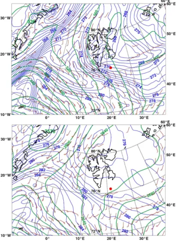
We report on results of a Polar-2 research flight which took place in the vicinity of Svalbard on 10 April 2007 between 11:05 and 13:59 UTC. The area where the cloud was ob-served is indicated in Fig. 1. At this time, cold Arctic air influenced Svalbard whereas the warm sector of an east-ward propagating trough dominated the wind field west of the islands. Thus, the near-surface south-easterly winds were weak and mostly aligned with the Arctic frontal zone as shown by the equivalent potential temperature distribu-tion and the wind field at the pressure surface of 925 hPa in Fig. 1a. At higher altitudes, the weak geopotential height
Fig. 1. ECMWF operational analyses: Equivalent potential
tem-perature (blue contour lines, K), geopotential height (green contour lines, m), and wind speed (barbs, m s−1) valid at 10 April 2007, 12:00 UTC at 925 hPa (a) and at 700 hPa (b). The position of the sampled ice cloud is marked by a red dot.
gradients and the absence of upper-level forcing caused a weak south-westerly flow over Svalbard; cf. the flow field at 700 hPa in Fig. 1b. The wind speed and direction measured during the flight at the altitude of the cloud were 4.5 m s−1 and 253◦, respectively. The operational European Centre of Medium Range Weather Forecasting (ECMWF) analyses charts reveal a north-south oriented band of increased relative humidity over ice (RHI) over Svalbard (Fig. 2). In the region of the airborne observations, RHI attained values of ≈90% at 700 hPa. Operational forecasts used for the flight plan-ning predicted cirrus at higher altitudes. In the operational analyses valid at 12:00 UTC, a formerly coherent region of RHI ≈100% was perturbed by ascending upper tropospheric air leading to smaller RHI values in the measurement area, cf. RHI at p=400 hPa in Fig. 2. The air temperature was measured during the flight with a Rosemount-PT100 sensor and corrected for the dynamic heating effect. In the cloud it-self (at 683 hPa), a mean temperature of −24.3◦C was found. During ascent and descent of the aircraft, a small temperature inversion of less than 2 K was found around 500 m above sea
Fig. 2. ECMWF operational analyses: Relative humidity (blue
shading, yellow contour lines RHU>100%), and geopotential height (green contour lines, m), valid at 10 April 2007, 12:00 UTC at 400 hPa (a) and at 700 hPa (b).
level. The relative humidity related to water saturation inside the cloud was 79 (±10)%, measured with a Vaisala HMT333 detector. This corresponds to a relative humidity above ice of ≈100% (almost saturated).
The NOAA satellite image (Fig. 3) confirms the ECMWF analyses. An elongated band of cumulus clouds west of Svalbard marked the air mass boundary whereas the area south and south-east of Svalbard was almost free of low-level clouds. The near infrared channel of the NOAA satellite re-veals high-level cirrus clouds north of Svalbard and cirrus associated with the approaching warm front in accordance with the RHI values for 400 hPa as shown in Fig. 4.
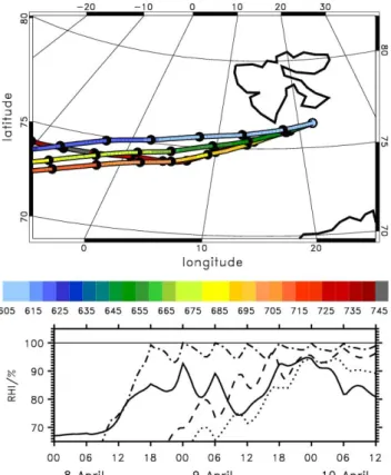
To examine the history of the observed air parcels, the three-dimensional trajectory model LAGRANTO (LA-GRangian ANalysis TOol, cf. Wernli and Davies, 1997) was applied. LAGRANTO is driven by the wind fields of the 6-hourly operational ECMWF analyses and allows the cal-culation of kinematic Lagrangian trajectories. Trajectories arriving between 600 and 750 hPa in the observational area at 10 April 2007 12:00 UTC reveal a slow propagation from
Fig. 3. NOAA satellite imagery on 10 April 2007, 11:21 UTC. Left
panel: visible channel (0.58–0.68 µm), right panel: near infrared channel (0.725–1.10 µm). Courtesy of the Norwegian Meteorolog-ical Institute, Tromsø, Norway.
south-west, see Fig. 4. In this altitude region, the absence of significant deformation and mixing indicates that the air mass kept its properties for the past 24 h. Before this time, the air parcels slowly ascended and, eventually, the relative humid-ity above ice increased to values close but below 100% in the global meteorological analyses. Trajectories arriving at 400 hPa were descending with decreasing RHI in time (not shown).
Fig. 4. Backward trajectories released at 21.8◦E and 76.4◦N on 10 April 2007 at 12:00 UTC. Top panel: Pressure along the trajectories for pstart=750, 700, 650, and 600 hPa, respectively. The black
bul-lets are plotted every 6 h. Bottom panel: relative humidity over ice RHI for pstart=750 (solid line), 700 (dotted line), 650 (dashed line),
and 600 (dash-dotted line) hPa, respectively.
The stable atmospheric conditions with low wind speeds continued in the same area (76.45◦–76.6◦N, 20.8◦-21.3◦E)
throughout the next day. During a CALIOP overflight on the next morning, 11 April at 09:53 UTC, an optically thin cloud at around 3 km altitude was recorded. The isobaric flow on this following day came from south-east without significant lift of the air masses in the last 24 h.
3 Airborne observations
Airborne observations of the subvisible Arctic ice cloud were performed in two consecutive stages. First, the lidar and ra-diation sensors detected the cloud from below as the aircraft flew eastwards at an altitude of 160 m above sea level be-tween 11:54 UTC and 12:09 UTC. The aircraft returned to the cloud center at an altitude of 2820 m as indicated by lidar remote sensing. There, the ice cloud layer was probed di-rectly by in situ instruments (12:28 UTC to 12:34 UTC). Tak-ing into account the advection of the air durTak-ing the 30 min be-tween the lidar detection and the in situ observation, the air-craft could not probe exactly the same air masses. However,
due to the almost stationary atmospheric conditions, we are confident that we indeed observed the same cloud.
3.1 Lidar remote sensing
The Airborne Mobile Aerosol Lidar (AMALi) deployed on-board the Polar-2 aircraft is a backscatter lidar system oper-ating at the two wavelengths λ=355 nm and λ=532 nm, re-spectively. Furthermore, the volume depolarization is mea-sured at one wavelength (λ=532 nm). For ASTAR 2007, the optical system and data acquisition of the original setup by Stachlewska et al. (2004) were modified. A new wavelength (355 nm instead of 1064 nm) and detectors measuring in both analogue and photon counting mode were implemented, the latter in order to increase the measurement range. AMALi can be installed either in nadir-looking or zenith-looking con-figuration. During the flight of the case study presented here, the lidar was deployed in zenith-looking mode. The vertical resolution of the system is 7.5 m. The horizontal resolution along the flight track depends on integration time and ground speed of the aircraft. In order to obtain a sufficiently high sig-nal to noise ratio (SNR) larger than 15 for the 532 nm chan-nel at the cloud top, the data were averaged over 15 s. With a mean ground speed of the aircraft of 62 m s−1, the horizontal resolution of the lidar data amounts to about 930 m.
The backscattering ratio BSR for a given wavelength λ is defined as
BSR(λ, z) = β
Ray(λ, z) + βpart(λ, z)
βRay(λ, z) , (1)
where βRay and βpart are the molecular Rayleigh and the particle backscatter coefficients, respectively. The air den-sity profiles necessary for estimating βRay were computed from meteorological data of the radiosonde launched at 11:00 UTC in Ny- ˚Alesund, Svalbard.
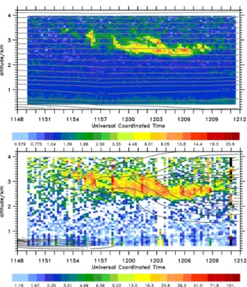
The vertical profiles of the backscattering ratio (532 nm) along the flight track reveal the presence of an optically thin ice cloud from 11:52 UTC to 12:09 UTC as shown in Fig. 5a. The geometrical depth varied between 500–1000 m. The cloud base was located at about 2500 m and the cloud top descended along the flight track from 3500 m to 3000 m al-titude. After 12:00 UTC, a cirrus cloud was recorded above the optically thin ice cloud at an altitude of 6–6.5 km (not shown in Fig. 5a).
The particle backscatter coefficient βpart for λ=532 nm as calculated with the standard Klett approach (Klett, 1985; Ansmann et al., 1992) exhibits values between 0.3(±0.1)*10−6m−1sr−1 and 5(±1)×10−6m−1sr−1 throughout the cloud. The lidar ratio LR, defined as the ratio of particle extinction coefficient αpart and particle backscatter coefficient
LR(z, λ) = α
part(z, λ)
βpart(z, λ), (2)
is set to 21 sr as a preliminary first guess, which is a typi-cal value for ice clouds (Ansmann et al., 1992; Giannakaki
Fig. 5. Backscatter ratio at 532 nm smoothed vertically about 3
height steps (m−1sr−1, top panel) and volume depolarization (%, bottom panel) with 15 s resolution along the flight track of the Polar-2 as indicated in Fig. 1. Large values of the depolarization with an extension in vertical bands are artefacts. Superimposed are contour lines of the potential temperature (K, top) and the cloud ice water content (mg kg−1, bottom). Meteorological data: ECMWF opera-tional analyses interpolated in space and time on the flight track.
et al., 2007). For the calculation of the particle backscatter coefficient, the assumed LR is not critical: The Arctic atmo-sphere apart from the subvisible cloud was so clear that Klett solutions with different LR were very similar to each other (with errors less than 2%). The minimum resolution for the particle backscatter coefficient of the AMALi is in the range of (1±0.5)×10−7m−1sr−1.
However, for calculating the extinction coefficient, the assumption of the lidar ratio is crucial (cf. discussion in Sect. 4.3). Assuming a lidar ratio of 21 sr, the extinc-tion coefficient in the cloud varied between 0.006 and 0.1(±0.003) km−1. The error of the extinction coefficient was estimated according to error propagation with reason-ably chosen uncertainties of βpart and LR. The uncertainty of LR was assumed as the magnitude of LR itself, 21 sr. As the small values of the backscatter coefficient have the highest relative error, we used the minimum resolution value (1×10⁻⁷m−1sr−1) for the error in backscatter coefficient. The uncertainty in the retrieval of the extinction coefficient thus amounts to 3×10⁻³km−1.
Furthermore, we calculated the cloud optical thickness τ at λ=532 nm by integrating the extinction coefficient from an altitude of 2100 m (zb) to 3735 m (zt): τ = zt Z zb α(z)dz0= zt Z zb LR · β(z)dz0 (3)
The values varied from subvisible (0.01–0.03) for more than half of the observation time to an upper value of 0.09(±0.005). After visual inspection of all lidar profiles and as expected due to the low optical depth τ <0.1 (You et al., 2006), multiple scattering can be excluded for this case.
To obtain information about the particle shape and cloud phase, we analyzed the volume depolarization (Fig. 5b). Below the cloud, the depolarization signal had low values around 1.4%, typical for air molecules (free troposphere with low aerosol load). The signal showed significantly enhanced values allover the cloud with values up to 40%. This clearly indicates the existence of non-spherical ice crystals in the ob-served subvisible midlevel ice cloud (You et al., 2006).
In order to estimate the size of the cloud particles, we ad-ditionally analyzed the color ratio Cpartas used by Liu and Mishchenko (2001) which is defined as
Cpart(z) = (4)
BSR(532 nm, z) − 1 BSR(355 nm, z) − 1 =
βpart(532 nm, z) × βRay(355 nm, z)
βpart(355 nm, z) × βRay(532 nm, z).
From the definition of the color ratio, the limit for very small particles (size of molecules) is Cpart=1 as the parti-cle backscatter coefficients for both wavelengths converge to the Rayleigh backscatter coefficients and the terms cancel in Eq. (4). For “large” particles in the regime of geometrical optics, the limit is Cpart≈5 as βpart(532 nm)=βpart(355 nm). In the sense of the two lidar wavelengths, “large” refers to particles with an effective diameter exceeding 5 µm (size pa-rameter larger than 40).
The entire cloud exhibited values of the color ratio of 3 to 4, demonstrating the existence of particles with an effective diameter smaller than 5 µm. As this is an ill-posed prob-lem, a precise retrieval of the particle size is impossible with the two lidar wavelengths only. Such small cloud particles with a size smaller than 5 µm and very low concentration are also difficult to detect directly with the in situ sensors (see Sect. 3.2).
3.2 In situ measurements
The center of the subvisible midlevel ice cloud was probed with the in situ instrumentation at the altitude of 2820 m, fol-lowing the guidance from the lidar measurements collected 30 min earlier. During this flight sequence, microphysical data were obtained between 12:29 and 12:34 UTC.
The independent in situ instruments used for this analysis include the Polar Nephelometer (PN, Gayet et al., 1997), the Cloud Particle Imager (CPI, Lawson et al., 1998) and the Forward Scattering Spectrometer Probe (FSSP-100, Dye and Baumgardner, 1984; Gayet et al., 2007).
The PN measures the scattering phase function of an en-semble of cloud particles (from about 3 µm to about 800 µm diameter), which intersect a collimated laser beam near the focal point of a parabolic mirror. The light scattered at an-gles from about 3.5◦ to 173◦ is reflected onto a circular ar-ray of 56 near-uniformly positioned photodiodes (in this case study reliable measurements were performed at 34 angles ranging from about 6.7◦ to 155◦). The laser beam is pro-vided by a high-power (0.8 W) multimode laser diode oper-ating at a wavelength of 804 nm. The data acquisition sys-tem is designed to provide a continuous sampling volume by integrating the measured signals of each of the detec-tors over a manually-defined period. Methods have been developed to infer the particle phase (liquid or ice), optical parameters (asymmetry parameter, volume extinction coeffi-cient, extrapolated phase function at 532 nm, and lidar ratio), and microphysical properties (particle size distribution, liq-uid water content (LWC), ice water content (IWC), and par-ticle number concentration). An iterative inversion method developed by Oshschepkov et al. (2000) and upgraded by Jourdan et al. (2003a), using physical modeling of the scat-tered light, is applied to the average angular scattering coef-ficients (ASC) measured by the PN in the subvisible Arctic ice cloud. The retrieval method and results are discussed in detail in Sect. 4.1. The average errors of the measurements of the angular scattering coefficients lie between 3% to 5% for scattering angles ranging from 15◦to 155◦(with a
maxi-mum error of 20% at 155◦) (Shcherbakov et al., 2006). The
uncertainties of the derived extinction coefficient and asym-metry parameter from PN measurement are estimated to be in the order of 25% and 5% respectively (Gayet et al., 2002). Only 4 single ice crystals were recorded with the CPI dur-ing the measurement time, which had column shape with a length of 100–200 µm (Fig. 6). The rounded edges of the ice crystals suggest that the cloud was in an evaporation pro-cess (see Sect. 2). The very few ice crystals detected indi-cate that (i) the particle concentration was very low and (ii) most of the ice crystals evidenced by the PN were smaller than about 100 µm. Furthermore, the FSSP did not detect particles. This means that the concentration of ice crys-tals with a size smaller than 50 µm was below the instru-ment’s detection threshold at the aircraft airspeed, i.e. about 0.2 cm−3. The low concentration was confirmed by the
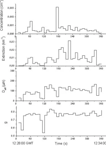
anysis of the PN data, which measured single ice crystals al-though the instrument was designed to probe an ensemble of cloud particles. Therefore, assuming the detection of single particles and knowing the sampling volume (150 cm3with a true airspeed of 70 m s−1at 20 Hz), the ice particle concen-tration can be estimated from the extinction coefficient and the effective diameter. The time series (every 10 s) of these
Fig. 6. Images of the four single ice crystals detected by the CPI in
the thin cloud at about 3 km altitude.
quantities together with the asymmetry parameter g defined as g =<cos θ >= 1 2 1 Z −1
cos θ × P (cos θ ) × d cos θ (5)
are displayed in Fig. 7 with θ being the scattering angle and
P the phase function. If there were several particles in the sampling volume, the effective diameter would be overes-timated and the concentration underesoveres-timated. Integrating the PN data over the 4 min cloud sequence, the mean val-ues of the extinction coefficient and asymmetry parameter are 0.01 km−1and 0.78, respectively, and the concentration of ice particles and mean effective diameter are 0.5 l−1 and
100 µm, respectively. For averaging over the densest part of the cloud (30 s), the extinction coefficient and an asymmetry parameter are 0.02 km−1and 0.77, respectively.
3.3 Radiation measurements
The Spectral Modular Airborne Radiation measurement sysTem (SMART)-Albedometer developed by Wendisch et al. (2001) was configured to measure upwelling and down-welling radiance and irradiance. For airborne applications, the optical inlets are mounted on an active horizontal stabi-lization platform. The six grating spectrometers coupled to the optical inlets provide data both in the visible (VIS, 350– 1000 nm) and near infrared (NIR, 1000–2150 nm) wave-length ranges with a spectral resolution of 2–3 nm and 9– 16 nm respectively, and a temporal resolution of 1 Hz in the VIS, 2 Hz in the NIR. The system is described in detail by Wendisch et al. (2001) and Ehrlich et al. (2008). In the case of the optically thin ice cloud investigated in this study, we analyzed the downwelling nadir radiance Iλ↓, which is most sensitive to the slightly enhanced scattered solar radiation be-low the cloud. The overall uncertainty of Iλ↓was estimated with 6% at the wavelength of 532 nm.
Fig. 7. Time series of the concentration, extinction coefficient,
ef-fective diameter Deff, and asymmetry parameter g retrieved from the polar nephelometer.
Additionally, pyrgeometer measurements (Eppley instru-ments) of upwelling and downwelling thermal infrared ir-radiance were performed. Unfortunately, the pyrgeometer could not be adjusted perfectly due to space limitations (in-clination of around 5◦) and was not temperature stabilized. The data were used qualitatively only to identify if changes in the modeled data in this spectral range were appropriate.
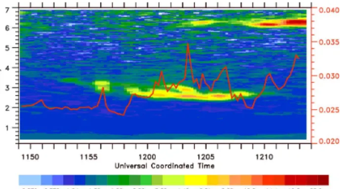
The downwelling radiance Iλ↓ measured during the lidar detection of the cloud showed a clear evidence of optically thin clouds above. Enhanced scattering of solar radiation by the cloud particles increased Iλ↓ as shown by the time se-ries in Fig. 8 (superimposed red line). The clear sky value of 0.025 W m−2sr−1nm−1at 532 nm was measured shortly
before the lidar detected the optically thin cloud. Simulta-neous with the increasing lidar backscatter ratio, also I532 nm↓ increased to a maximum value of 0.030 W m−2sr−1nm−1. From 12:00 UTC the cirrus detected by the lidar at 6– 6.5 km altitude lead to a further increase of I532 nm↓ up to 0.036 W m−2sr−1nm−1.
The response of the downwelling thermal infrared irradi-ance (pyrgeometer measurements) qualitatively had a similar
Fig. 8. Backscatter ratio at 532 nm smoothed vertically about 3
height steps with 15 s resolution as in Fig. 5. Superimposed is the radiance in W sr−1m−2nm−1 at 532 nm (red line). After 12:00 UTC, a cirrus cloud appears at an altitude of about 6 km.
behavior as the solar radiance and lidar optical thickness (not shown). Below the ice cloud the pyrgeometer values in-creased simultaneously with the lidar optical thickness from values of 172 W m−2 to 176 W m−2. After 12:00 UTC, the
additional cirrus cloud above the optically thin ice cloud lead to further increased values measured by the pyrgeometer.
4 Discussion
4.1 Microphysical properties
The inversion method for the PN data is based on a bi-component representation of cloud composition and consti-tutes a non-linear least square fitting of the scattering phase function using smoothness constraints on the desired particle size distributions (PSD). Measurement errors at each angle and PSD’s values for each size, in a sense of probability den-sity function, are assumed to be described by the lognormal law, which is the most natural way to take a priori informa-tion about the non-negativity of these quantities (Tarantola, 1994). Note that no analytical expression for the particle size distribution is assumed for the converging solution in this method. The only constraint in this connection is smooth-ness, needed to avoid an unrealistic jagged structure of the desired size distribution, because the inverse problem is ill posed without constraints. The inversion method is designed for the retrieval of two volume particle size distributions si-multaneously, in our case one for hexagonal ice columns and another for spherical ice crystals. The technique needs, how-ever, to specify a lookup table containing the scattering phase functions of individual ice crystals. Lookup tables contain-ing the angular scattercontain-ing coefficients of spherical ice crys-tals, droxcrys-tals, columns with three aspect ratios (2, 5, 10), plates with 4 aspect ratios (0.1, 0.5, 0.2, 1), hollow columns, 6 branch bullet rosettes, and aggregates were calculated.
Three roughness parameters for ice particles were also considered (smooth, moderately rough, and deeply rough).
The roughness of the surface can be defined as a small scale property similar to surface texture. In the simulation, the rough surface is assumed as composed of a number of small facets which are locally planar and randomly tilted from their positions corresponding to the case of a perfectly plane sur-face. The tilt distribution is supposed to be azimuthally ho-mogeneous. It is specified by a two parametric probabil-ity distribution function including a scale parameter σ and the shape parameter η (which determines the kurtosis). The model of surface roughness used in this paper is based on the Weibull statistics (Dodson, 1994) and was already proposed by Shcherbakov et al. (2006). This approach incorporates the Cox and Munk model used by Yang and Liou (1998). Sur-face roughness can substantially affect the scattering proper-ties of a particle if the geometric scale of the roughness is not much smaller than the incident wavelength. In the case of ra-diation scattered by large ice crystals (i.e. for size parameters within the geometric optics regime), surface roughness can reduce or smooth out the scattering peaks in the phase func-tion that correspond to halos. For the deeply rough case the computed phase function is essentially featureless. The 22◦ and 46◦ halos are smoothed out and the backscattering is substantially reduced because of the spreading of the colli-mated beams. We chose a roughness scale parameter σ =0.25 which is according to the Improved Geometric Optic Model (IGOM) considered as deeply rough.
In this case study, we tested all the possible combinations of the habits listed above.
The best fit of the measurement was achieved using a com-bination of spherical ice particles with diameters ranging from 1 µm to 100 µm and deeply rough hexagonal columns (with an aspect ratio of 2) with maximum dimension ranging from 20 µm to 900 µm. This model gives the smallest root mean square deviation compared with the measured ASC. Accordingly, two particle size distributions were retrieved. Since the inverse problem is ill posed for one specific com-bination of ice crystal geometry, different size distributions can be retrieved. This is accounted for in the estimation of the lidar ratio and the bulk microphysical parameters. The scattering phase function of spherical ice crystals was sim-ulated from Lorentz-Mie theory, and the scattering patterns of rough hexagonal column crystals randomly oriented in 3-D space were computed by an improved geometric-optics model (Yang and Liou, 1996). The bulk microphysical (num-ber concentration, IWC, effective diameter) and optical pa-rameters (volume extinction, extrapolated scattering phase function at 532 nm and lidar ratio) were assessed following the method presented by Jourdan et al. (2003b). On the ba-sis of the two particle size distributions, we calculated the extrapolated ASC in the forward and backward directions at the lidar wavelength (532 nm) as well as the extinction co-efficient. This step was performed using direct modeling of light scattering corresponding to the retrieved PSD. There-fore, we have access to both terms needed for the lidar ratio computation, namely the scattering coefficient at 180◦ and
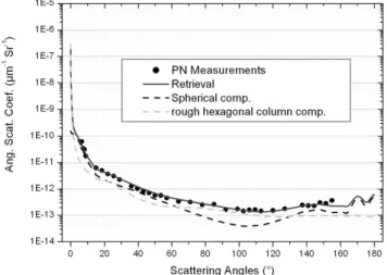
Fig. 9. Retrieved angular scattering coefficients at the Polar
Neph-elometer nominal wavelength (800 nm). Contributions of both com-ponents (ice spheres and ice columns) on the cloud total scattering properties are also displayed.
the extinction coefficient at 532 nm. From this method a LR of 27 sr with 25% error was estimated.
The retrieved ASC from the inversion scheme along with direct PN measurement are displayed in Fig. 9. The mea-sured ASC are flat at the side scattering angles, which is in accordance with most of the observations (Francis et al., 1999; Shcherbakov et al., 2005; Gayet et al., 2006; Jourdan et al., 2003b) or directions in ice cloud remote sensing ap-plication (see among others Labonnote et al., 2001; Baran and Labonnote, 2006, 2008; Baran and Francis, 2004). Scat-tering phase functions of non-spherical ice crystals mostly exhibit enhanced sideward scattering compared to spherical water droplets.
Figure 9 highlights that the retrieved ASC are in good agreement with PN direct measurements. The minimum root mean square deviation (15%) between the measured and the retrieved ASC was achieved for a microphysical model representing a combination of ice spheres and deeply rough hexagonal columns of aspect ratio equal to 2 (with maximum dimension of the crystals ranging from 1 to 100 µm and 20 to 900 µm, respectively). The scattering contribution of each microphysical component (dashed lines in Fig. 9) points out that the hexagonal ice crystal component reproduces the gen-eral flat behaviour of the measured ASC at side scattering angles. Roughness of the ice crystal mantle removed spe-cific optical features (22◦and 46◦halos, bows) linked to the hexagonal geometry of ice crystal. However, a small ice sphere component is needed to model the relatively higher scattering in the angular range [15◦–60◦] and [130◦–155◦] in comparison with hexagonal shape assumption.
The comparison of the model with direct microphysical measurements is limited in this case study, as only 4 sin-gle ice crystals were recorded by the CPI and no
statisti-cally significant measurements were performed by the FSSP-100. However, the CPI images (Fig. 6) suggest the presence of rounded edge column ice crystals with an average length of 100–200 µm. This observation supports the choice of a rough column component in the microphysical model. Ad-ditionally, as shown in Table 1, the retrieved effective diam-eter and number concentration of the hexagonal ice crystal component are acceptable compared to the measurements (effective diameter of 106 µm and very low concentration of 0.002 cm−3). As mentioned above, a small spherical ice component is needed in order to fit the measured ASC. The only information derived from direct measurements that could confirm the presence of small ice crystals is linked to the minimum detection threshold of the CPI and FSSP-100 instruments. The CPI is not able to detect particle with sizes lower than 10 µm (Lawson et al., 2001) and the FSSP-100 minimum measurable concentration is around 0.2 cm−3.
The microphysical retrievals are in agreement with the instru-ments shortcomings, as the estimated total number concen-tration of the ice cloud is 0.2 cm−3and the effective diameter of the small ice crystals is 4.5 µm.
In conclusion, a microphysical model composed of small spherical ice particles and larger deeply rough hexagonal col-umn crystals leads to optical and, to a certain extent, mi-crophysical properties (asymmetry parameter, extinction and ASC), which allows to reproduce the measurements. The low asymmetry parameter (∼0.78) of the PN measurements is consistent with the enhanced depolarization measurements of up to 40% and the CPI images indicating non-spherical ice crystals. It is not possible to distinguish the particle shape from the values of lidar depolarization measurements, not even for clouds composed entirely of one kind of ice par-ticle habits, as was evidenced by Monte Carlo simulations of You et al. (2006). Most of the asymmetry parameter values fall within the range that is typical of cirrus clouds shown by Gayet et al. (2006), i.e., a cloud containing ice particles was sampled. For spherical water droplets the asymmetry parameter is about 0.85, significantly larger than the values reported here.
The extinction coefficients retrieved from the PN range be-tween the lidar values (Sect. 3.1) but could not exhibit the maximum of 0.1 km−1measured by the lidar. This indicates that the aircraft was not within the densest part of the cloud during the in situ measurements, or the cloud generally was in the process of dissolving. The values of RHI around satu-ration and the round edges of the ice crystals confirm that dissolving processes were taking place in the cloud. The extinction coefficients are much below the typical values of midlatitude cirrus clouds as presented in Gayet et al. (2006). This clearly indicates that a subvisible midlevel ice cloud was probed.
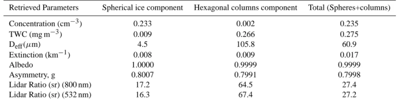
Table 1. Total retrieved bulk microphysical and single scattering properties from PN measurements and contribution of both components.
Retrieved Parameters Spherical ice component Hexagonal columns component Total (Spheres+columns)
Concentration (cm−3) 0.233 0.002 0.235 TWC (mg m−3) 0.009 0.266 0.275 Deff(µm) 4.5 105.8 60.9 Extinction (km−1) 0.008 0.009 0.017 Albedo 1.0000 0.9999 0.9999 Asymmetry, g 0.8007 0.7991 0.7998 Lidar Ratio (sr) (800 nm) 17.2 64.5 27.4 Lidar Ratio (sr) (532 nm) 16.3 67.4 27.2
Fig. 10. Top: Spectral downwelling radiance Iλ↓simulated (dashed lines) and measured (solid lines) by the SMART-Albedometer for clear sky conditions (black lines) and the observed optically thin midlevel ice cloud (blue lines). The measured and simulated data of the thin cloud are averaged over two minutes (indicated by ver-tical lines in the time series of Fig. 11). Bottom: Ratio between simulated and measured downwelling radiance for the clear sky and cloudy case.
4.2 Simulation of the measured radiation
The measured Iλ↓was employed to retrieve the optical thick-ness of the observed cloud. For this purpose, radiative trans-fer simulations were performed with the libRadtran package (Mayer and Kylling, 2005) using the DISORT version 2 ra-diative transfer solver by Stamnes et al. (1988). First the cloud free situation (11:50-11:52 UTC) was simulated, and then the subvisible midlevel ice cloud was included in order to match the observations between 11:53 and 12:00 UTC.
To accurately reproduce the clear sky downwelling radi-ance, measured before the subvisible cloud appeared above the aircraft, a cirrus cloud approaching from the South and later also detected by the lidar had to be considered. During the first part, the cirrus was not directly above the aircraft
but already in front of the sun affecting the diffuse sky radia-tion. The cirrus optical properties, optical depth τ =0.04 and effective radius Reff=60 µm, were estimated as best fit to the
measured clear sky radiance and included in the simulations by using the parameterization of Key et al. (2002) assuming solid column ice crystals. The spectral downwelling radi-ance of clear sky simulations and measurements shown in Fig. 10 (black lines) are in good agreement especially for the wavelength range between 500 nm and 600 nm, including the 532 nm channel (vertical bar) of AMALi.
In a second step, the subvisible cloud was included in the simulations. The scattering phase function and single-scattering albedo were derived from the PN measurements as described in Sect. 4.1. The simulations for a solar zenith angle of 70◦were found to be robust against the chosen
scat-tering phase function. For the scatscat-tering angle of 70◦ the scattering phase function shows almost the same values for all shapes of ice crystals. Therefore the simulations are most sensitive to the cloud optical thickness τ . By variation of
τ, the simulations were modified in order to fit the mea-surements of Iλ↓below the cloud. The spectral downwelling radiance simulated below the subvisible cloud is shown in Fig. 10 as blue line. From this method an optical thickness of 0.048 was obtained for the time interval between 11:53 and 12:00 UTC. The mean spectral downwelling radiance shown as dashed line agrees well with this simulation.
The ratio between simulated and measured downwelling radiance ranges between ±10% for most wavelengths (Fig. 10, lower part). As the simulations were fitted by vary-ing the cloud optical depth, the best agreement was found at 532 nm wavelength. The deviations at other wavelengths result from a) uncertainties of the spectrometer and b) the aerosol optical depth assumed for the radiative transfer sim-ulations. The aerosol optical depth applied to the simulations was scaled by the ˚Angstrom formula with an ˚Angstrom expo-nent of α=1.51 and an aerosol optical thickness at 1µm wave-length of τ =0.03. Both coefficients were obtained from sun photometer measurements at Ny- ˚Alesund on 7 April 2007 using a SP1A sun photometer (Herber et al., 2002). As the airborne measurements were conducted about 370 km away
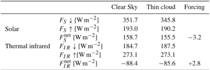
Table 2. Modeled downwelling and upwelling irradiance and net
fluxes in the solar and thermal infrared wavelength range.
Clear Sky Thin cloud Forcing Solar FS↓[W m−2] 351.7 345.8 FS↑[W m−2] 193.0 190.2 FSnet[W m−2] 158.7 155.5 −3.2 Thermal infrared FI R↓[W m−2] 184.7 187.5 FI R↑[W m−2] 273.1 273.1 FI Rnet[W m−2] −88.4 −85.6 +2.8
from Ny- ˚Alesund, a different aerosol optical thickness may have been present in the vicinity of the subvisible cloud. However, as Fig. 10 shows, the ratio between measurements and simulations is similar for the cloud free and cloudy case. This implies that variations in the SMART-Albedometer data (cloud free, cloudy) result only from changes of the cloud properties and not from aerosol properties. The scattering properties of cloud particles in the visible wavelength range are almost independent of the wavelength, whereas aerosol scattering decreases exponentially with a power law with in-creasing wavelength in this wavelength range.
Although the differences between clear sky and cloud cov-ered case were low, the simulations showed that the radiative effects of the optically thin cloud were detectable by the ra-diance measurements.
4.3 Lidar ratio
The lidar ratio is crucial for determining the extinction co-efficient and the cloud optical depth τ from lidar measure-ments (cf. Eqs. 2 and 3). As the extinction coefficient and the cloud optical depth are proportional to the lidar ratio, the two quantities are strongly influenced by the error of the lidar ratio. Therefore, three independent methods of determining the lidar ratio are applied and compared in the following.
4.3.1 PN measurements
On the basis of the microphysical model described in Sect. 4.1, the corresponding ASC for a wavelength of 532 nm was computed in order to derive the ice cloud mean lidar ratio. The extrapolated scattering phase function of the PN delivered relatively high lidar ratios, depending on the as-sumed particle shape. The best agreement of the model and the measured extrapolated scattering phase function was ob-tained with a lidar ratio of 27(±7) sr. This resulted from fit-ting a mixture of small ice spheres, and deeply rough hexag-onal columns with an aspect ratio of 2 to the scattering phase function. The relative error of 25% accounts for instrumental errors and extrapolation technique.
4.3.2 Transmittance method
Another independent approach to determine the effective li-dar ratio is the transmittance method (Chen et al., 2002). From the elastic lidar profiles themselves, the lidar ratio can be estimated: Assuming the same backscattering ratio BSR below and above the cloud, the extinction in the cloud can be calculated by solving the elastic lidar equation
P (z)z2 = Cρ(z)BSR(z) exp (−2
z
Z
0
α(z0)dz0), (6)
with the lidar signal P (z), the density ρ(z), the extinction coefficient α(z), and C representing a system constant. We used the signals at the wavelength λ=532 nm. As the cloud was located at an altitude in the free troposphere on a day without pollution (indicated by the clear sky values of optical depth measured with the lidar directly before the cloud), the assumption of the same backscattering ratio is justified.
Hence, if BSR(zb) ≡BSR(zt)for the height of the cloud
bottom zband top zt, respectively, it follows:
BSR(zb) = P (zb) z2b Cρ(zb) exp(+2 zb Z 0 α(z0)dz0) = (7) BSR(zt) = P (zt) z2t Cρ(zt) exp(+2 zb Z 0 α(z0)dz0)exp(+2 zt Z zb α(z0)dz0)
From Eq. (7), the extinction in the cloud (between zband
zt) can be determined. According to Nicolas et al. (1997),
this value constitutes an upper limit, as diffraction leads to enhanced apparent optical depths. The inspection of the lidar signal led to the estimation that multiple scattering did not decrease the LR by more than 2 sr, which is included in our error bars.
The elastic lidar Eq. (6) is then solved by the standard Klett approach (see Sect. 3.1 for errors). The LR is varied to best fit the cloud extinction resulting from Eq. (7) for each time step. We retrieved 6 single values and their error bars for the LR with a horizontal resolution of 930 m between 11:54 and 12:00 UTC. The mean effective value for the cloud was found to be 15 (±10) sr.
4.3.3 Combination of lidar and radiation measurements
From SMART-Albedometer measurements, a time series of the cloud optical depth was retrieved for the lidar wave-length of 532 nm. For this purpose, the method described in Sect. 4.2 was applied systematically. Lookup tables were cal-culated for the downwelling radiance I532 nm↓ assuming cloud optical thickness in the range of 0–0.5. For each measure-ment of the SMART-Albedometer, an appropriate value of
Fig. 11. Time series of cloud optical thickness determined from
SMART-Albedometer measurements (black line) and from lidar data for different values of the lidar ratio (27, 21 and 15 sr, colored lines). The error bars at exemplary time steps display the uncer-tainty of the albedometer retrieval. The vertical bars indicate the time interval over which the measured and simulated values were averaged for the spectra shown in Fig. 10.
the measured I532 nm↓ . Fig. 11 shows a time series of τ re-trieved from I532 nm↓ . In addition, the cloud optical thick-nesses derived from AMALi assuming three different LR (PN measurements LR=27 sr, mean value LR=21 sr, transmittance method LR=15 sr) are given. In general, the derived τ agree within the uncertainty range of τ retrieved from the SMART-Albedometer until 11:59 UTC. After 12:00 UTC the cirrus cloud was above the aircraft increasing the measured radi-ance. Therefore, τ retrieved from the SMART-Albedometer overestimates the optical thickness of the subvisible cloud.
Assuming that single scattering (at a scattering angle of 70◦) is dominating the radiative transfer through the
subvis-ible cloud, τ is obtained independent of the ice crystal scat-tering phase function (and LR). The retrieved τ are used in combination with the AMALi measurements to derive an in-dependent estimate of the LR. By dividing τ by the corre-sponding integral of the particle backscatter coefficient, the
LR is calculated (see Eq. 3). For the time when the cloud
was detected without cirrus above, and omitting the cloud free section around 11:57 UTC, this method resulted in an effective LR of 20 (±10) sr.
4.3.4 Comparison
In summary, we determined the effective lidar ratio and its er-ror bar by three independent methods (evaluation of PN data, transmittance method applied to lidar data , and combination of cloud optical thickness derived from albedometer and in-tegrated lidar backscatter) in order to estimate the value and the accuracy of this parameter. A LR of 27(±7) sr was
ob-tained from the PN data, 15(±10) sr from the transmittance method, and 20(±10) sr from the combined albedometer and lidar data. The mean lidar ratio calculated from these three values by error propagation amounts to 21 sr. The error bar was estimated according to the following considerations: A lidar ratio in the range of 20 to 25 sr is within the error bars of all measurements. We also included the mean values of the LR obtained by the in situ retrieval and the transmittance method in the range of the LR. As an overall lidar ratio, we propose 21(±6) sr. This value is in reasonable agreement with other LR values for cirrus clouds in the literature (Ans-mann et al., 1992; Chen et al., 2002; Cadet et al., 2005; Gi-annakaki et al., 2007).
4.4 Cloud radiative forcing
Broadband solar and infrared, downwelling and upwelling ir-radiance (FS ↓, FS ↑, FI R ↓, FI R ↑) were calculated at
air-craft altitude for two cases. First, the observed situation in-cluding the subvisible midlevel ice cloud and the cirrus cloud above (case 1) was simulated using the input parameters as described in Sect. 4.2. The net solar irradiance FSnet=FS ↓
−FS ↑was found to be FSnet=155.5 W m
−2, the net thermal
infrared irradiance FI Rnet=FI R ↓ −FI R ↑=−85.6 W m−2. To
estimate the radiative forcing of the subvisible midlevel ice cloud, a second simulation including only the cirrus cloud was evaluated (case 2). Without the midlevel ice cloud, the net solar irradiance increases to FSnet= 158.7 W m−2, while the net thermal infrared irradiance is reduced to
FI Rnet=−88.4 W m−2 (Table 1). The solar radiative forcing of the subvisible midlevel ice cloud (case 1 minus case 2) of −3.2 W m−2indicates enhanced reflection of solar radi-ation due to the subvisible cloud. On the other hand, the surface cooling by emission of infrared radiation from the surface layer was reduced by about 2.8 W m−2(thermal in-frared forcing of the subvisible midlevel ice cloud). There-fore, the net effect of the cloud on the local radiation budget was a slight cooling effect of −0.4 W m−2. On a local scale in which the subvisible cloud was observed, this cooling is almost negligible.
The small net radiative effect estimated from the radiative transfer simulations was detected by the radiation ments only in certain limits. The solar irradiance measure-ments did not show any response to the subvisible midlevel ice cloud. The measurement uncertainty of 4% exceeds the estimated changes in FS↓and FS ↑(2% change).
The increased downwelling thermal infrared radiation re-lated to the presence of the optically thin cloud was ob-served by the pyrgeometer, which showed an increase from 172 W m−2to 176 W m−2. The magnitude of the change is consistent with the simulations, which calculated an increase from 184.7 W m−2 to 187.6 W m−2. The disagreement of the absolute values can be attributed to the reasons given in Sect. 3.3.
5 Conclusions
The atmospheric radiative energy budget in the Arctic cru-cially depends upon cloud cover (Curry et al., 1996). Even optically thin, subvisible ice clouds may contribute to a local warming or cooling, depending on their microphysical prop-erties, the surface albedo and the solar zenith angle. During the ASTAR 2007 campaign, we were able to probe a sub-visible midlevel ice cloud with a lidar, different in situ and radiation sensors. Based on the data obtained by the polar nephelometer, albedometer and backscatter lidar, we simu-lated the cloud’s effect on the solar and thermal infrared ra-diation. Furthermore, the cloud microphysical and optical properties were characterized. A mean cloud optical depth of 0.048 was estimated from the measured downwelling ra-diance. With the measurement uncertainty of the SMART-Albedometer (≤6%), this values agrees well with the cloud optical depth calculated from the AMALi data.
Based on three independent methods, we analyzed the val-ues of the lidar ratio for the optically thin ice cloud. Com-bining all three methods, a LR of 21(±6) sr matches to all measurements in the best way. The lidar ratio is mainly de-termined by the shape of the individual ice crystals. The phase function determined by the polar nephelometer was best fit assuming a mixture of ice spheres with a mean size of 4.5 µm, and deeply rough columns, which were probed by the CPI. The small spheres were not detected directly during our flight. For the in situ detection by FSSP, the particles were too small and the concentration too low. The lidar color ratio indicates the existence of particles smaller than 5 µm.
The radiative forcing of the optically thin midlevel ice cloud was estimated by simulations using the retrieved op-tical properties. For the solar spectrum, the opop-tically thin mi-dlevel ice cloud had a cooling effect of −3.2 W m−2whereas for the thermal infrared spectral range, the cloud exhibited a warming effect of 2.8 W m−2. The net radiative effect was a slight cooling of −0.4 W m−2. Although this small value is generally negligible – especially on a local scale – under night time conditions without solar forcing, the net warming effect of such a cloud is substantial.
Compared to Arctic aerosol layers, the radiative effects of Arctic clouds are often in the same order of magnitude (Blanchet and List, 1983; Rinke et al., 2004), but sometimes with the opposite sign. Arctic haze, often occurring at the same altitudes as the optically thin midlevel ice cloud ana-lyzed here (Scheuer et al., 2003), is generally warming the atmosphere (Blanchet and List, 1983). A further effect of subvisible midlevel ice clouds in the free troposphere might be the interaction with aerosols. Here, the aerosols act as ice condensation nuclei and the cloud as a sink for aerosols. The study of Jiang et al. (2000) shows that the existence of Arctic mixed-phase clouds is very sensitive to the concentration of ice forming nuclei. It is likely that similar interactions take place with midlevel subvisible clouds. More investigations
are necessary to confirm and quantify these possible impli-cations.
Compared to cirrus clouds at higher altitudes with a simi-lar optical depth, the optically thin midlevel ice cloud of this study shows a generally higher IR forcing due to the higher temperatures at lower altitudes. Thus, midlevel Arctic ice clouds tend to cool the surface temperatures less than higher ice clouds with comparable optical properties in the solar wavelength range.
The repeated occurrence of atmospheric conditions favor-able for the formation of optically thin midlevel Arctic ice clouds is suggested by the CALIOP observation of a similar thin cloud in the same region one day later on 11 April. This emphasizes the relevance of this cloud type for the Arctic radiative budget.
For the time period of the ASTAR 2007 campaign (26 March to 16 April 2007), the data of 113 overpasses of the CALIOP lidar were available for the geographical location around Svalbard (0–30◦E, 75–82◦N). In 62 of these cases, clouds were found in the height range of 2.5 to 3.5 km that were optically thin enough that the lidar signal was not com-pletely attenuated but penetrated to the ground. Cases with boundary layer clouds beneath were not considered. Al-though this is only a very rough estimate, it underlines the possible importance of thin midlevel clouds. Even if these clouds have a small effect on the radiation budget as for the case presented here, their existence could be important in the Arctic winter, when the thermal warming effect is not bal-anced by the cooling influence in the solar wavelength range. A detailed analysis of the frequency of occurrence of this cloud type in winter, e.g. using the CALIOP data set, is be-yond the scope of this paper.
Acknowledgements. The CALIPSO data were provided by the
NASA Langley Research Center Atmospheric Science Data Cen-ter. Andreas D¨ornbrack acknowledges the reliable access to the ECMWF forecast and analysis data through the Special Project “In-fluence of non-hydrostatic gravity waves on the stratospheric flow field above Scandinavia”. This research was partly funded by the German Research Foundation (DFG, WE 1900/8-1).
The authors would like to thank the three anonymous reviewers for their suggestions and comments, which helped us to improve the structure and content of the manuscript.
Edited by: T. Garrett
References
Ansmann, A., Wandinger, U., Riebesell, M., Weitkamp, C., and Michaelis, W.: Independent measurement of extinction and backscatter profiles in cirrus clouds by using a combined Raman elastic-backscatter lidar, Appl. Opt., 31, 33, 7113–7131, 1992. Baran, A. J. and Francis, P. N.: On the radiative properties of cirrus
cloud at solar and thermal wavelengths: A test of model consis-tency using high-resolution airborne radiance measurements, Q. J. Roy. Meteor. Soc., 130, 763–778, 2004.
Baran, A.J., and Labonnote L.-C.: On the reflection and polarisation properties of ice cloud, J. Quant. Spectrom. Rad. T., 100, 41–54, 2006.
Baran, A. J. and Labonnote L.-C.: A self-consistent scattering model for cirrus. I: The solar region, Q. J. Roy. Meteor. Soc., 133, 1899–1912, 2008.
Beyerle, G., Gross, M. R., Haner, D. A., Kjome, N. D., McDermid, I. S., McGee, T. J., Rosen, J. M., Sch¨afer, H.-J., and Schrems, O.: A Lidar and Backscatter Sonde Measurement Campaign at Table Mountain during February-March 1997: Observations of Cirrus Clouds, J. Atmos. Sci., 58, 1275–1287, 2001.
Blanchet, J.-P. and List, R.: Estimation of optical properties of Arc-tic haze using a numerical model, Atmos. Ocean, 21, 444–464, 1983.
Cadet B., Goldfarb, L., Faduilhe, D., Baldy, S., Giraud, V., Keck-hut, P., and R´echou, A.: A sub-tropical cirrus clouds climatology from Reunion Island (21◦S, 55◦E) lidar data set, GRL 30, 3, 1130, doi:10.1029/2002GL016342, 2003.
Cadet, B., Giraud, V., Haeffelin, M., Keckhut, P., R´echou, A., and Baldy, S.: Improved retrievals of the optical properties of cir-rus clouds by a combination of lidar methods, Appl. Opt., 44(9), 1726–1734, 2005.
Chen, W. N., Chiang, C. W., and Nee, J. B.: Lidar ratio and de-polarisation ratio for cirrus clouds, Appl. Opt., 31, 6470–6476, 2002.
Cox, C. and Munk, W.: Measurement of the roughness of the sea surface from photographs of the sun’s glitter, J. Opt. Soc. Amer., 44, 838–850, 1954.
Curry, J. A. and Ebert, E. E.: Annual Cycle of Radiation Fluxes over the Arctic Ocean: Sensitivity to Cloud Optical Properties, J. Clim., 5, 1267–1280, 1992.
Curry, J. A., Rossow, W. B., Randall, D., and Schramm, J. L.: Overview of Arctic Cloud and Radiation Characteristics, J. Clim., 9, 1731–1764, 1996.
Dodson, B.: Weibull Analysis, Milwaukee, Wisconsin: ASQC, 256 pp., 1994.
Dye, J. E. and Baumgardner, D.: Evaluation of the Forward Scat-tering Spectrometer Probe. Part I: Electronic and optical studies, J. Atmos. Ocean. Technol., 1, 329–344, 1984.
Ehrlich, A., Bierwirth, E., Wendisch, M., Gayet, J.-F., Mioche, G., Lampert, A., and Heintzenberg, J.: Cloud phase identification of Arctic boundary-layer clouds from airborne spectral reflection measurements: test of three approaches, Atmos. Chem. Phys., 8, 7493–7505, 2008.
Francis, P. N., Foot, J. S., and Baran A. J.: Aircraft measurements of the solar and infrared radiative properties of cirrus and their dependence on ice crystal shape, J. Geophys. Res., 104, 31685– 31696, 1999.
Gayet, J.-F., Cr´epel, O., Fournol, J. F., and Oshchepkov, S.: A new airborne polar Nephelometer for the measurements of optical and microphysical cloud properties. Part I: Theoretical design, Ann. Geophys., 15, 451–459, 1997,
http://www.ann-geophys.net/15/451/1997/.
Gayet, J.-F., Auriol, F., Minikin, A., Str¨om, J., Seifert, M., Kre-jci, R., Petzold, A., Febvre, G., and Schumann, U.: Quan-titative measurement of the microphysical and optical proper-ties of cirrus clouds with four different in situ probes: Evi-dence of small ice crystals, Geophys. Res. Lett., 29, 24, 2230, doi:10.1029/2001GL014342, 2002.
Gayet, J.-F., Shcherbakov, V. N., Mannstein, H., Minikin, A., Schu-mann, U., Str¨om, J., Petzold, A., Ovarlez, J., and Immler, F.: Microphysical and optical properties of midlatitude cirrus clouds observed in the southern hemisphere during INCA, Q. J. Roy. Meteor. Soc., 132, 621, 2719–2748, 2006.
Gayet J.-F., Stachlewska, I. S., Jourdan, O., Shcherbakov, V., Schwarzenboeck, A., and Neuber, R.: Microphysical and opti-cal properties of precipitating drizzle and ice particles obtained from alternated Lidar and in situ measurements, Ann. Geo., 25, 1487–1497, 2007.
Giannakaki, E., Balis, D. S., Amiridis, V., and Kazadzis, S.: Opti-cal and geometriOpti-cal characteristics of cirrus clouds over a mid-latitude lidar station, Atmos. Chem. Phys., 7, 5519–5530, 2007, http://www.atmos-chem-phys.net/7/5519/2007/.
Harrington, J. Y., Reisin, T., Cotton, W. R., and Kreidenweis, S. M.: Cloud resolving simulations of Arctic stratus, Part II: Transition-season clouds, Atmos. Res., 51, 45–75, 1999.
Herber, A., Thomason, L. W., Gernandt, H., Leiterer, U., Nagel, D., Schulz, K.-H., Kaptur, J., Albrecht, T., and Notholt, J.: Continuous day and night aerosol optical depths observations in the Arctic between 1991 and 1999, J. Geophys Res. 107(D10), doi:10.1029/2001JD000536, 2002.
Immler, F. and Schrems, O.: Lidar observations of extremely thin clouds at the tropical tropopause, Reviewed and revised papers presented at the 23rd International Laser Radar conference 24– 28 July 2006, Nara, Japan, edited by: Nagasawa, C. and Nobuo Sugimoto, I., 547–550, 2006.
Immler, F., Kr¨uger, K., Fujiwara, M., Verver, G., Rex, M., and Schrems, O.: Correlation between equatorial Kelvin waves and the occurrence of extremely thin ice clouds at the tropical tropopause, Atmos. Chem. Phys., 8, 4019–4026, 2008,
http://www.atmos-chem-phys.net/8/4019/2008/.
Intrieri, J. M. and Shupe, M. D.: Characteristics and radiative ef-fects of diamond dust over the western Arctic Ocean region, J. Clim., 17(15), 2953–2960, 2004.
Inoue, J., Liu, J., Pinto, J. O., and Curry, J. A.: Intercomparison of Arctic Regional Climate Models: Modeling Clouds and Radia-tion for SHEBA in May 1998, J. Clim., 19, 4167–4178, 2006. Jiang, H., Cotton, W. R., Pinto, J. O., Curry, J. A., and Weissbluth,
M. J: Cloud Resolving Simulations of Mixed-Phase Arctic Stra-tus Observed during BASE: Sensitivity to Concentration of Ice Crystals and Large-Scale Heat and Moisture Advection, J. At-mos. Sci., 57, 2105–2117, 2000.
Jourdan, O., Oshchepkov, S., Gayet, J.-F., Shcherbakov, V. N., and Isaka, H.: Statistical analysis of cloud light scattering and microphysical properties obtained from airborne measurements, J. Geophys. Res., 108(D5), 4155, doi:10.1029/2002JD002723, 2003a.
Jourdan, O., Oshchepkov, S., Shcherbakov, V., Gayet, J.-F., and Isaka, H.: Assessment of cloud optical parameters in the so-lar region: Retrievals from airborne measurements of scat-tering phase functions, J. Geophys. Res., 108(D18), 4572, doi:10.1029/2003JD003493, 2003b.
Key, J. R., Yang, P., Baum, B. A., and Nasiri, S. L.: Param-eterization of shortwave ice cloud optical properties for vari-ous particle habits, J. Geophys. Res.-Atmos., 107(D13), 4181, doi:10.1029/2001JD000742, 2002.
King, M. D., Platnick, S., Yang, P., Arnold, G. T., Gray, M. A., Riedi, J. C., Ackerman, S. A., and Liou, K.-N.: Remote
Sens-ing of Liquid Water and Ice Cloud Optical Thickness and Effec-tive Radius in the Arctic: Application of Airborne Multispectral MAS Data, J. Atmos. Ocean. Technol., 21, 857–875, 2004. Klett, J. D.: Lidar inversions with variable backscatter/extinction
values, Appl. Opt., 24, 1638–1648, 1985.
Labonnote, L.-C., Brogniez, G., Buriez, J.-C., Doutriaux-Boucher, M., Gayet, J.-F., and Macke, A.: Polarized light scatter-ing by inhomogeneous hexagonal monocrystals : Validation with ADEOS-POLDER measurements, J. Geophys. Res., 106, 12139–12154, 2001.
Lawson, P., Heymsfield, A. J., Aulenbach, S. M., and Jensen, T. L.: Shapes, sizes and light scattering properties of ice crystals in cirrus and a persistent contrail during SUCCES, Geophys. Res. Lett., 25, 1331–1334, 1998.
Lawson, R. P., Baker, B. A., Schmitt, C. G., and Jensen, T. L.: An overview of microphysical properties of Arctic clouds ob-served in May and July 1998 during FIRE ACE, J. Geophys. Res., 106(D14), 14989–15014, 2001.
Liu, L. and Mishchenko, M. I.: Constraints on PSC particle micro-physics derived from lidar observations, J. Quant. Spectros. Rad. T., 70, 817–831, 2001.
Masuda, K., Kobayashi, T., Raschke, E., Albers, F., Koch, W., and Maixner, U.: Short-wave radiation flux divergence in Arctic cir-rus: a case study, Atmos. Res., 53, 251–267, 2000.
Mayer, B. and Kylling, A.: Technical note: The libRadtran software package for radiative transfer calculations – description and ex-amples of use, Atmos. Chem. Phys., 5, 1855–1877, 2005, http://www.atmos-chem-phys.net/5/1855/2005/.
McGill, M. J., Vaughan, M. A., Trepte, C. R., Hart, W. D., Hlavka, D. L., Winker, D. M, and Kuehn, R. Airborne validation of spa-tial properties measured by the CALIPSO lidar, J. Geophys. Res., 112, D20201, doi:10.1029/2007JD008768, 2007.
Nicolas, F., Bissonnette, L. R., and Flamant, P. H.: Lidar effec-tive multiple-scattering coefficients in cirrus clouds, Appl. Opt., 36(15), 3458–3468, 1997.
Oshchepkov, S. L., Isaka. H., Gayet, J. F., Sinyuk, A., Auriol, F., and Havemann, S.: Microphysical properties of mixed-phase & ice clouds retrieved from in situ airborne “Polar Nephelometer” measurements, Geophys. Res. Lett., 27, 209–213, 2000. Peter, T., Luo, B. P., Wirth, M., Kiemle, C., Flentje, H., Yushkov,
V. A., Khattatov, V., Rudakov, V., Thomas, A., Borrmann, S., Toci, G., Mazzinghi, P., Beuermann, J., Schiller, C., Cairo, F., Di Donfrancesco, G., Adriani, A., Volk, C. M., Strom, J., Noone, K., Mitev, V., MacKenzie, R. A., Carslaw, K. S., Trautmann, T., San-tacesaria, V. and Stefanutti, L.: Ultrathin Tropical Tropopause Clouds (UTTCs): I. Cloud morphology and occurrence, Atmos. Chem. Phys., 3, 1083–1091, 2003.
Rinke, A., Dethloff, K., and Fortmann, M.: Regional climate effects of Arctic Haze, Geophys. Res. Lett., 31, L16202, doi:10.1029/2004GL020318, 2004.
Sassen, K., Griffin, M. K., and Dodd, G. C.: Optical Scattering and Microphysical Properties of Subvisual Cirrus Clouds, and Climatic Implications, J. Appl. Meteorol., 28, 91–98, 1989. Scheuer, E., Talbot, R. W., Dibb, J. E., Seid, G. K., and DeBell, L.:
Seasonal distributions of fine aerosol sulfate in the North Ameri-can Arctic basin during TOPSE, J. Geophys. Res. 108(D4), 8370, doi:10.1029/2001JD001364, 2003.
Schweiger, A. J., Lindsay, R. W., Key, J. R., and Francis, J. A.: Arctic Clouds in Multiyear Satellite Data Sets, J. Geophys. Res., 26(13), 1845–1848, 1999.
Shcherbakov, V. N., Gayet, J.-F., Jourdan, O., Minikin, A., Str¨om, J., and Petzold, A.: Assessment of Cirrus Cloud Optical and Mi-crophysical Data Reliability by Applying Statistical Procedures, J. Atmos. Ocean. Technol., 22(4), 409–420, 2005.
Shcherbakov, V. N, Gayet, J.-F, Baker, B., and Lawson, P.: Light Scattering by Single Natural Ice crystals, J. Atmos. Sci., 63, 1513–1525, 2006.
Shupe, M. D. and Intrieri, J. M.: Cloud radiative forcing of the Arctic surface: The influence of cloud properties, surface albedo and solar zenith angle, J. Clim., 17, 616–628, 2004.
Spichtinger, P., Gierens, K., and D¨ornbrack, A.: Formation of ice supersaturation by mesoscale gravity waves, Atmos. Chem. Phys., 5, 1243–1255, 2005,
http://www.atmos-chem-phys.net/5/1243/2005/.
Stachlewska, I. S., Wehrle, G., Stein, B., and Neuber, R.: Airborne Mobile Aerosol Lidar for measurements of Arctic aerosols, Proceedings of 22nd International Laser Radar Conference (ILRC2004), ESA SP-561, 1, 87–89, 2004.
Stamnes, K., Tsay, S., Wiscombe, W., and Jayaweera, K.: A nu-merically stable algorithm for discrete-ordinate-method radiative transfer in multiple scattering and emitting layered media, Appl. Opt., 27, 2502–2509, 1988.
Tarantola, A.: Inverse problem theory: Methods for data fitting and model parameter estimation, 2nd imp., Elsevier Sci., Am-sterdam, The Netherlands, 601 pp., 1994.
Thomas, A., Borrmann, S., Kiemle, C., Cairo, F., Volk, M., Beuer-mann, J., Lepuchov, B., Santacesaria, V., Matthey, R., Rudakov, V., Yushkov, V., MacKenzie, A. R., and Stefanutti, L.: In situ measurements of background aerosol and subvisible cirrus in the tropical tropopause region, J. Geophys. Res., 107(D24), 4763, doi:10.1029/2001JD001385, 2002.
Vaughan, M., Young, S., Winker, D., Powell, K., Omar, A., Liu, Z., Hu, Y., and Hostetler, C.: Fully automated analysis of space-based lidar data: An overview of the CALIPSO retrieval algo-rithms and data products, Proc. SPIE Int. Soc. Opt. Eng., 5575, 16–30, 2004.
Wendisch, M., M¨uller, D., Schell, D., and Heintzenberg, J.: An air-borne spectral albedometer with active horizontal stabilization, J. Atmos. Ocean. Technol., 18, 1856–1866, 2001.
Wernli, H. and Davies, H. C.: A Lagrangian-based analysis of ex-tratropical cyclones, I: The method and some applications, Q. J. Roy. Meteor. Soc., 123, 467–489, 1997.
Winker, D. M., Hunt, B. H., and McGill, M. J.: Initial perfor-mance assessment of CALIOP, Geophys. Res. Lett., 34, L19803, doi:10.1029/2007GL030135, 2007.
Yang, P. and Liou, K. N., Geometric-optics-integral-equation method for light scattering by nonspherical ice crystals, Appl. Opt., 35, 6568–6584, 1996.
Yang, P. and Liou, K. N.: Single scattering properties of complex ice crystals in terrestrial atmosphere, Contr. Atmos. Phys., 71, 223–248, 1998
You, Y., Kattawar, G. W., Yang, P., Hu, Y. X., and Baum, B. A.: Sensitivity of depolarized lidar signals to cloud and aerosol par-ticle properties, J. Quant. Spectr. Rad. T., 100, 470–482, 2006.