The memory of fluctuating brownian dipolar chains

(1)

HAL Id: hal-00107356

https://hal.archives-ouvertes.fr/hal-00107356

Submitted on 9 Nov 2018

HAL is a multi-disciplinary open access

archive for the deposit and dissemination of

sci-entific research documents, whether they are

pub-lished or not. The documents may come from

teaching and research institutions in France or

abroad, or from public or private research centers.

L’archive ouverte pluridisciplinaire HAL, est

destinée au dépôt et à la diffusion de documents

scientifiques de niveau recherche, publiés ou non,

émanant des établissements d’enseignement et de

recherche français ou étrangers, des laboratoires

publics ou privés.

Renaud Toussaint, Eirik Grude Flekkøy, Geir Helgesen

To cite this version:

Renaud Toussaint, Eirik Grude Flekkøy, Geir Helgesen. The memory of fluctuating brownian dipolar

chains. Physical Review E : Statistical, Nonlinear, and Soft Matter Physics, American Physical Society,

2006, 74 (5), pp.051405. �10.1103/PhysRevE.74.051405�. �hal-00107356�

(2)

Memory of fluctuating Brownian dipolar chains

Renaud Toussaint,1,*Eirik G. Flekkøy,2 and Geir Helgesen3

1_{Institute of Globe Physics in Strasbourg (IPGS), UMR 7516 CNRS, 5 rue Descartes, F-67084 Strasbourg Cedex, France} 2

Department of Physics, University of Oslo, P.O. Box 1048 Blindern, NO-0316 Oslo, Norway

3

Institute for Energy Technology, NO-2027 Kjeller, Norway 共Received 19 June 2006; published 20 November 2006兲

Nonmagnetic particles in suspension in a ferrofluid act as magnetic holes when an external magnetic field is exerted: They acquire an effective dipolar moment opposing the surrounding one, which induces dipolar magnetic interactions. For a large enough imposed field and particle size, the induced interactions dominate the thermal forces, dipolar chains form. At equilibrium, these chains fluctuate under the effect of brownian noise. When the imposed magnetic field is suddenly decreased, these chains roughen dynamically. We study the time and size scaling of these fluctuations and roughening, and the relationships between the equilibrium and out of equilibrium behavior. We compare the experimental data both to Brownian dynamics simulations, and to a simple theory of semiflexible polymer chains, a generalization of the Rouse model. The scaling behavior of the experiments agree with the predictions of both theory and simulations over 5 orders of magnitudes. The roughening follows three successive regimes: The root mean square width of the chain initially evolves as W⬃t1/2_{, then it enters a subdiffusive regime where W}_⬃t1/4_{and eventually it saturates to a level W}_{⬃N, where}

N is the number of particles in the chain. The exact prefactors as a function of the applied field, particle diameter, and temperature are also derived analytically. We also show that this phenomenon can be described equivalently as a non-Markovian diffusion process for a particle in an environment with memory effects. Within this framework, our system is shown to confirm the predictions of theories for anomalous diffusion in systems with memory.

DOI:10.1103/PhysRevE.74.051405 PACS number共s兲: 82.70.Dd, 75.50.Mm, 05.40.⫺a, 83.10.Pp

I. INTRODUCTION

When micrometer sized nonmagnetic spheres are sus-pended in a magnetized ferrofluid they define magnetic holes that interact very much like magnetic dipoles 关1–3兴. These

dipole interactions may be precisely controlled by the exter-nal field. In 1983, Skjeltorp introduced such a system that allowed direct observation by the use of transparent glass plates and perfectly monodisperse Ugelstad spheres关4兴.

A population of magnetic holes may be brought to orga-nize in a rich variety of structures through their induced di-pole interactions关2兴. One of the simplest equilibrium

struc-tures that can be obtained, is a straight dipolar chain. When the particles are sufficiently small such chains exhibit lateral thermal fluctuations. We have recently described these fluc-tuations and shown that dipolar chains, or Brownian worms, are described by the Rouse model关5,6兴 for polymer

dynam-ics. Since hydrodynamic interactions between different chain segments are suppressed by the boundaries the present sys-tem in fact realizes the Rouse model more closely than any free polymer, and to our knowledge, any comparable experi-mental system.

The external control of the interparticle forces allows us to study the roughening of an initially straight chain. We study this dynamic process experimentally by optical micros-copy, and we compare it to Brownian dynamics simulations as well as analytical results. As a main result we observe growth exponents that agree well with the predictions 关5兴:

Initially the root-mean-square共rms兲 width of the chain grows

with a diffusive exponent of 1 / 2 which subsequently crosses over to an exponent of 1 / 4 before the chain width saturates at an asymptotic value that depends on the chain length. Analytically these exponents are derived from a discrete ver-sion of the Edwards-Wilkinson equation 关7兴—or

equiva-lently, the Rouse model.

Chain fluctuations in equilibrium are closely connected to the dynamic roughening process. We show that the dynamic roughening from an initially straight chain, and the departure from an initially rough state at equilibrium, are two equiva-lent problems, characterized by the same Family-Vicsek scal-ing with same roughness and dynamic exponents. Only the prefactor of the mean square chain width is different.

Having derived the discrete Edwards-Wilkinson equation with the coefficients corresponding to our experiment, we turn to an alternative theoretical description by which we identify the dynamic roughening as a process of anomalous diffusion关8兴. The long memory effects that are a prerequisite

for any process of anomalous diffusion, stem from the propa-gation of perturbations along the chain, and we compute the observed anomalous diffusion exponent of 1 / 4.

In general, the lateral fluctuations of dipolar chains have attracted much attention over the past two decades. The sys-tems in which such chains have been studied include in par-ticular magnetorheological 关9–12兴 and electrorheological

共ER兲 suspensions. In these systems, the dipolar moment is fixed inside the particles, in contrast to the present system where the interactions of the nonmagnetic particles only re-flect the magnetization of the surrounding fluid. Much of the interest in electrorheological and magnetorheological fluids is based on their ability to form chains under application of an external field, thereby changing the rheology. Technologi-cally these effects may allow the development of dampers, *Electronic address: renaud.toussaint@eost.u-strasbg.fr

(3)

hydraulic valves, clutches or brakes 关13–17兴. Over time

chains may aggregate laterally due to their Brownian motion. These effects are analogous to the van der Waals interaction, and have been analyzed by Halsey and Toor as well as Mar-tin et al. 关18–21兴. Therefore, the precise quantification of

Brownian motion of a single isolated dipolar chain is an important compound to understand the larger scale aggrega-tion phenomena, whether this happens in magnetorheological 关22–24兴 or electrorheological 关21,25,26兴 fluids, or in systems

of magnetic holes关27,28兴.

The paper is organized as follows: in Sec. II, we describe the experimental system under study along with some basic theoretical considerations. In Sec. III, we derive discrete Edwards-Wilkinson equation and the dynamical scaling of a dipolar chain. In Sec. IV, we describe the numerical Brown-ian dynamic model designed to simulate the chain motion. In Sec. V, we compare the analytical, numerical, and experi-mental results for the dynamic chain roughening. In the fol-lowing section, we derive analytically the connections be-tween the out-of-equilibrium roughening problem, and the equilibrium fluctuations. Next, in Sec. VII, we derive the linear response function of the chain, and show how the dy-namic scaling may be understood in the theoretical frame-work of diffusion in systems with memory关8兴. The

conclu-sions are eventually summarized in Sec. VIII.

II. THEORETICAL BASIS AND THE EXPERIMENTAL SETUP

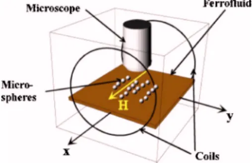
The magnetic properties of a ferrofluid stem from sus-pended magnetite particles which are of nanometer size. Therefore the magnetic properties of the ferrofluid is homo-geneous on the scale of the Ugelstad spheres. These spheres are of nonmagnetic polystyrene designed according to Ugel-stads technique关4兴. They are embedded in a kerosene-based

ferrofluid 关29兴 confined between two parallel glass plates

with a 10␮m separation共see Fig.1兲.

Since the Ugelstad spheres are not magnetized by the ex-ternal field they represent an effective dipole with a moment approximately equal to and opposite of the dipolar moment of the displaced ferrofluid. We are currently working to quantify this effective moment more precisely. However, to first approximation it may be written ␴= −V¯ H where␹ ␹ is the magnetic susceptibility of the ferrofluid, H the magnetic field, V is the holes volume and␹¯ = 3␹/共3+2␹兲 is an effec-tive susceptibility taking into account the demagnetization

factor associated with the spherical shape of the particles 关30兴. In the absence of confining walls the magnetic

interac-tion potential between two holes of diameter a, may be writ-ten关30兴 U =␮f␴ 2 4␲ 1 − 3 cos2␪ r3 , 共1兲

where r is the distance between the centers of the spheres, with a separation vector lying at an angle␪ to the external magnetic field. The ratio of the magnetic interaction energy to the thermal energy kT is denoted␭, and can be estimated from the above equation as关31兴

␭ = ␮f␴2

2␲a3kT=

␮f␹¯2H2␲a3

72kT . 共2兲

When␭ exceeds 1, the dipolar interactions lead the particles to organize in long chains parallel to the imposed field. At ␭Ⰷ1, these chains are essentially straight and rigid, and the particles are in contact. If the external field is suddenly re-duced to values that are still greater than 1, Brownian forces from the embedding fluid leads to a dynamic roughening of the chains共see Fig.2兲.

In the experiments the polystyrene spheres 关4兴, which

were of equal size, had diameters either a = 3.0 or 4.0␮m. They were dispersed in a kerosene-based ferrofluid 关29兴 of

susceptibility␹= 0.8 and viscosity␩= 6⫻10−3 _{Pa s, inside a}

glass cell of size 38 mm⫻8 mm⫻10␮m. A pair of outside coils produced a magnetic field parallel to the long axis of the cell with field strength up to H = 20 Oe. The setup was mounted under an optical microscope using an optical mag-nification of 20⫻ and having an attached video camera that recorded to a digital tape recorder at a speed of 25 frames per second. Low volume fractions 共1%兲 of microspheres were used and chains were grown by applying a constant field of about H = 18 Oe parallel to the thin ferrofluid layer for about 20 minutes关28兴. The cell was then searched for long chains

containing typically 20–120 spheres which were well sepa-rated from neighboring chains in order to avoid interchain interactions. The field was then reduced to a constant value H in the range 2 Oe艋H艋10 Oe while the motion of one long chain was recorded. The recorded video, which had a frame size of 720⫻576 pixels, was analyzed with a sam-pling rate of four frames per second. One pixel of the video image corresponded to 0.5␮m, and the uncertainty in par-ticle position could be reduced to 0.2␮m by utilizing the intensity profile of the pixels showing the particle. The initial roughness of the chains before reducing the field strength was less than the experimental resolution of 0.2␮m, and the time to reduce the magnetic field from the initial to the final value was about 1 s, thus introducing a similar uncertainty in the starting moment of free fluctuations. During an experi-ment the nonmagnetic particles were centered midway be-tween the upper and lower glass plate of the cell due to magnetic repulsion from the nonmagnetic walls 共the mag-netic “mirror image” effect兲关2兴. The experiments illustrated

in Fig. 2 are challenging in part because this accuracy is needed to reveal the scaling behavior of the chains.

(4)

III. ANALYSIS OF LATERAL FLUCTUATIONS

To obtain the dynamic description of the chain we start from the nearest neighbor interactions and consider depar-tures from the minimum energy configuration of the straight chain.

First we estimate the magnitude of next-nearest-neighbor interactions: From Eq.共1兲 we see that U⬀1/r3_{and therefore}

that the ratio of the nearest-neighbor energy to the energy associated with the remaining interactions may be written

U共a兲

兺

n=2 ⬁ U共na兲 ⬇ aU共a兲

冕

2a ⬁ drU共r兲 = 8. 共3兲

This we will take as justification to neglect interactions be-yond nearest neighbor ones.

To identify the equation of motion for the position hiof

particle i in the direction normal to the applied field, we perform a Taylor expansion of the magnetic interaction po-tential in Eq.共1兲 around the rigid chain reference state. This

gives the normal component of the magnetic force acting on sphere i as

Fi M

= k_⬜共hi+1− 2hi+ hi−1兲共4兲

with k_⬜=␲␮f¯␹2H2a/12, 共5兲

where a is the particle diameter, and H the external applied field. Typically a⬇3␮m, and H = 20 Oe, so that k_⬜⬇1.2 ⫻10−6_{kg/ s}2_.

Since the Reynolds number in this system is very small 共using the particle diameter a=1␮m and the thermal particle velocity, Re= 10−4_{兲 the hydrodynamic forces are linear in the}

particle velocity. Neglecting in a first stage the hydrody-namic interactions between the particles, we write then

Fi H

= − f_⬜hi, 共6兲

where f_⬜= 3␲␩a, with the fluid viscosity␩= 6⫻10−3 _{Pa s.}

We will comment further on the influence of the confining cell boundaries on this drag coefficient, and on the influence of the hydrodynamic coupling between the particles in the chain.

Newton’s second law for the ith sphere is then

mh¨共xi兲 = FM共xi兲 + FH共xi兲 + F˜i共t兲, 共7兲

where we have added also the fluctuating force F˜i共t兲, which

is due to the molecular nature of the fluid and gives rise to the Brownian motion of the particle.

The correlation time of F˜i共t兲 cannot exceed the viscous

damping time tm= m / f⬜. This is the time it takes for a

par-ticle velocity to decay. An upper bound for tmin our system

is given by tm= a2␳/ 18␩⬇5⫻10−6s, and above this time

scale we may assume

具F˜i共t兲F˜j共0兲典 = A␦共t兲␦ij, 共8兲

where A is a constant. In passing we note that since a force over a particle in general causes inertial motion in the fluid, that will decay only over a finite viscous damping time, the equation of motion for兵hi其 will also in general have a

non-Markovian nature, i.e., the motion of hiwill depend not only

the instantaneous forces but the entire history of those forces 关32,33兴. However, due to the presence of the confining plates

the damping time for any inertial motion is simply tm, and

above this time it is correct to neglect the non-Markovian corrections to Eq. 共7兲. This argument can also be given a

FIG. 2. Dynamic roughening of dipolar chains of magnetic holes of diameter 4␮m after a decrease of the external magnetic field from␭=866 to ␭=24 at t=0. 共a兲 Region with low density of chains,共b兲 the longest chain 10 s before the field was reduced 共t = −10 s兲, 共c兲 t=0, 共d兲–共h兲 t=3 s, 10 s, 30 s, 60 s, and 150 s, respec-tively.共i兲 Time evolution of the root-mean-square half-width of the chain.

(5)

more rigorous basis by showing that the non-Markovian in-terface equations, as given in Ref. 关32兴, actually reduces to

Eq.共7兲 in the tm→0 limit.

Having established the Markovian nature of our descrip-tion without this rigor we now determine A. The observadescrip-tion that F˜iis independent of FM allows us to determine A from

共7兲 with the FMterm removed. Following standard textbook

关34兴 procedures we multiply the remainder of Eq. 共7兲 by

exp关共f⬜/ m兲t兴 to obtain the explicit solution h˙共xi, t兲

=兰_−⬁t dt

⬘

1

Ⲑ

m F˜i共t

⬘

兲e关−共f⬜/m兲共t−t⬘兲兴. If we average the square of

this equation, use Eq.共8兲 and invoke the equipartition

prin-ciple we obtain kBT =具mh˙共xi兲2典=A/2f_⬜which gives

A = 2f_⬜kBT. 共9兲

Combining the above results, and neglecting the inertial terms due to the smallness of tm, Eq.共7兲 can be written

h˙i= k_⬜ f_⬜共hi+1+ hi−1− 2hi兲 + 1 f_⬜F ˜ i共t兲. 共10兲

This is a discrete form of the Edwards-Wilkinson equation, valid when␭Ⰷ1 where the quadratic approximation of the potential is valid. For spatial scales above a and times above tm, the above reduces to the Edwards-Wilkinson equation关7兴,

⳵h ⳵t = k_⬜a2 f_⬜ ⳵2_h ⳵x2 + 1 f_⬜F ˜ i共t兲, 共11兲

also known in polymer dynamics as the Rouse model关6兴.

A chain of particles may be made arbitrarily straight by applying large external magnetic fields. As an idealization of this situation we shall assume an initially straight chain and ask how it roughens when the external fields are reduced, while␭⬎1, which ensures that the chain does not melt and the Taylor expansion performed above is accurate enough. As a side result we shall also find the equilibrium width of the chain, that results as a balance between the Brownian forces that tends to buckle the chain and the magnetic forces that tend to straighten it out.

For this purpose we will take the discrete Fourier trans-form of Eq.共10兲 as a starting point. The Fourier transforms

are defined as hj= h共xj兲 =

兺

n=0 N−1 eiknxj_h n, hn= hk_n= 1 N

兺

j=0 N hje−iknxj, 共12兲 where xj= ja, j = 0,1, . . . ,N − 1, kn= 2␲ Nan, n = 0, . . . ,共N − 1兲. 共13兲 The Fourier transform of Eq.共10兲 may be written

h˙n= −␻nhn+ 1 f_⬜F ˜_n_, _共14兲 where ␻n= k_⬜ f_⬜2关1 − cos共kna兲兴. 共15兲 Equation共14兲 is easily solved to give

hn共t兲 = 1 f_⬜

冕

_−⬁ t dt

⬘

e−␻n共t−t⬘兲_F˜ n共t

⬘

兲共16兲

and correspondingly Eq.共8兲 takes the form—force:

具F˜n共t兲F˜n⬘

* _{共0兲典 =}2f⬜kBT

N ␦共t兲␦nn⬘. 共17兲 The mean square width W2 _{is defined as the average of} _共h

i

− 1 / N兺jhj兲2, which by Parseval’s identity may be written

W2= 1 N

兺

i

冓

冉

hi− 1 N

兺

j hj

冊

2

冔

=

兺

n⬎0 具兩hn兩2典. 共18兲

An initially straight particle chain is most conveniently described by setting F˜n共t⬍0兲=0. The average of the square

of hn共t兲 then takes the form

具兩hn共t兲兩2典 = 2kBT Nf_⬜

冕

₀ t dt

⬘

e−2␻n共t−t⬘兲共19兲 =2kBT f_⬜ 1 − e−2␻nt 2␻n 共20兲 and W2=2kBT Nf_⬜n

兺

艌1 1 − e−2␻nt 2␻n . 共21兲

When tⰆ1/␻maxwe have关1−exp共−2␻nt兲兴/共␻nt兲⬇2 and

W2⬇2kBT

f_⬜ t. 共22兲

This result arises only because of the existence of a shortest wavelength a in the system. In the continuum limit a→0,

␻max→⬁, and the tⰆ1/␻maxregime does not exist. Equation

共22兲 describes the superposition of N independent random

walks in the h direction, and therefore the t1/2_{dependence of}

W is as expected.

When 1 /␻maxⰆtⰆ1/␻min, then ␻ktⰇ1 for large k and

␻ktⰆ1 for small k. Since 关1−exp共−2␻nt兲兴/共␻nt兲 is of order

1 for the smallest␻kand关1−exp共−2␻nt兲兴/共␻nt兲Ⰶ1 for large

␻kwe see that the sum over wave numbers is dominated by

the small ␻k. We can then write ␻k⬇共ka兲2/␶ where ␶

= f_⬜/ k_⬜⬇0.2共H/20 Oe兲2s. By noting that ␻N−n=␻n, the

mean square width W2 may be cast in the Family-Vicsek scaling form关35兴

W2= LF

冉

t

L2

冊

, 共23兲

(6)

F共x兲 = kBT 2␲2k_⬜a

兺

_n=1

N/2

1 − e−8k⬜a2_␲2n2x/f_⬜

n2 . 共24兲

This equation has the following physical interpretation. Every mode kngrows to its equilibrium value on a time scale

1 /␻n. At that point there is an equilibrium between the

ef-fects of the thermal force F˜i and the restoring force FM_i.

Since at small times W must be independent of L and at large times, when W has reached its asymptotic value, it must be independent of t, we have that

F共x兲 ⬃

再

x

1/2 _{for small x,}

const for large x.

冎

共25兲 From this it follows that

W⬃

再

t

1/4 _{for small t,}

L1/2 for large t.

冎

共26兲 To get the prefactors however, we must evaluate the sums. In the 1 /␻_maxⰆtⰆ1/␻_minregime we can replace the sum by an integral to a good approximation. This yields

n=1 N/2 1 ␻n ⬇ kBT 2␲2k_⬜ L a

兺

n=1 ⬁ 1 n2. 共30兲 Using J = 1 2␲2

兺

n=1 ⬁ 1 n2= 1 12 共31兲

we may summarize the above as

W2= kBT

冦

2 f_⬜t when tⰆ 1 ␻max ,

冑

2 ␲k_⬜f_⬜t 1/2 _when 1 ␻max Ⰶ t Ⰶ 1 ␻min , 1 12k_⬜ L a when tⰇ 1 ␻min .

冧

共32兲

Noting finally from Eqs.共13兲 and 共15兲 that 1/␻max=␶/ 4

and 1 /␻_min= N2_␶_{/ 4}_␲2_{, those separation times can be}

evaluated as 1 /␻max= 0.06共H/20 Oe兲2 s and 1 /␻min

= N2· 0.06共H/20 Oe兲2 s.

IV. BROWNIAN DYNAMIC SIMULATIONS

The dynamic roughening of such dipolar chain can also be studied numerically by performing Brownian dynamics simulations. In this model the interaction forces, which act on each particle of the chain, is composed of the dipole-dipole interaction of Eq.共1兲, a repulsive contact force, and a

thermal, fluctuating force from the surrounding fluid. Such a numerical study allows us to study the effects neglected in the analytical derivation above, namely,共1兲 the finite range of the dipolar interactions beyond nearest neighbor ones.共2兲 The influence of the nonlinearities in the potential for large departures from a straight chain.共3兲 The fact that particles are not constantly in contact but have somewhat fluctuating spacings.

Our hydrodynamic regime is strongly damped, which im-plies that the acceleration term mir¨ is negligible compared to

the viscous friction term Fv= −f_⬜r˙i. The time evolution of

each particle in the chain is then given by the force-balance equation

f_⬜r˙i= −

冉

兺

j

Fm共rj− ri兲

冊

+ Fc共rj− ri兲 + F˜i共t兲, 共33兲

where the magnetic interaction force is derived from the pair potential U in Eq.共1兲, i.e., Fm共r兲=−ⵜU.

The contact forces are modeled as

Fc共r兲 = f0⌰共a − r兲rˆ exp

冉

r − a l −

l

r − a

冊

, 共34兲 where⌰ is a Heavyside function, r−a the overlap distance between neighboring particles, l a characteristic distance of overlap, rˆ the radial unit vector, and f0 the characteristic

force magnitude arising from the elastic properties of the particle material. The shape of this interaction is chosen so that this force and its derivative of any order are continuous—although similar results are obtained with the simpler form Fc共r兲= f0⌰共a−r兲rˆ exp关共r−a兲/共l兲兴. In the

model, we adopt arbitrarily l = 0.01a, and f0= U共r=a,␪

= 0兲/a. By testing several values of these parameters, we have checked that these particular values are irrelevant for the roughening dynamic, as long as l / aⰆ1, which ensures that the interactions approximate those of rigid particles.

The hydrodynamic interactions between the plates and the particles cannot be neglected. They are taken into account in the following way.

Since the magnetic interactions between the particles and the nonmagnetic boundaries keep the particles in the middle between the plates, the hydrodynamic coupling between the particles and the plates amount to increasing the friction co-efficient by a factor

c = 2/共1 − 9a/16d兲 − 1 = 1.40共1.70兲 共35兲 for a = 3␮m共4␮m兲关36兴. Consequently, the viscous friction

(7)

the hydrodynamic interactions between the particles are ne-glected, as will be justified further in Sec. V B.

The magnitude of the fluctuating force in the Langevin equation, Eq. 共33兲, is set up by the fluctuation-dissipation

theorem, as derived in Eqs.共9兲, i.e.,

具F˜i共t兲F˜j共0兲典 = 2f⬜kBT␦共t兲␦ij. 共36兲

The Langevin equation 共33兲 is directly integrated over

time steps⌬t as f_⬜关ri共t + ⌬t兲 − ri共t兲兴共37兲 = −

冉

兺

j Fm关rj共t兲 − ri共t兲兴

冊

⌬t 共38兲 + Fc关rj共t兲 − ri共t兲兴⌬t + ⌬F˜ i共t兲, 共39兲

where according to the central limit theorem and Eq.共36兲,

the integrated random variables ⌬F˜ i=兰tt+⌬tF˜i共t

⬘

兲dt

⬘

are

un-correlated Gaussian variable of zero mean and of variance given by

具⌬F˜

i共t兲⌬F˜ j共t⬘兲典 = 2f⬜kBT⌬t␦tt⬘␦ij. 共40兲

The time step⌬t is chosen so that the average spatial steps do not exceed 0.001 diameters. The simulations are run from an initial state where all particles are in contact and aligned. As in the experiments, under the effect of thermal noise, the chains roughen until they reach a characteristic fluctua-tion size. The equilibrium size of these fluctuafluctua-tions depend on the applied field. Five snapshots of a typical simulation are shown in Fig.3, together with an experiment carried out with similar field parameters. In the experiment, the field was reduced from a strong value corresponding to␭=866, to a lower one corresponding to␭=24. In the simulation, the ini-tial straight state corresponding to ␭Ⰷ1 is let to fluctuate according to the Brownian dynamic scheme carried out with restoring magnetic forces at␭=24. The visual agreement be-tween simulations and experiments seems satisfying, as shown in Fig.3.

V. COMPARISON BETWEEN THEORETICAL MODEL, SIMULATIONS AND EXPERIMENTS

A. Evolution of the chain width

To characterize the roughening dynamic of the dipolar chains, we extract the root-mean-square width of the lateral coordinates as function of time t after a decrease of the ex-ternal field from a strong value. Since this system is excited by thermal noise, this width differs between realizations. We record this width as a function of time for each single ex-periment or numerical realization of Brownian dynamics simulation,

Wsr共t兲 =

1 N

兺

j

hj2 共41兲

The average over realizations of this rms width should correspond to the thermodynamic average W共t兲=具Wsr典

de-rived in Sec. III. In order to check the scaling law dede-rived in Eq.共32兲, for the width as function of time, we plot the scaled

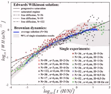
width WH

冑

a / N as function of the scaled time, tc共H/N兲2, in Fig.4. Each symbol represents a different experiment, with a different applied field, particle number or particle diameter, as specified in the figure.

The black continuous lines correspond to the predicted thermodynamic average, evaluated from Eq. 共32兲 with f_⬜

= 3c␲␩a with c given by Eq. 共35兲. The dashed lines

corre-spond to the initial freely diffusive regime for chains of length 36, 59, and 122. The data collapse of the experimental data in these reduced coordinates is consistent with the ana-lytical model, but the scatter around the thermodynamic av-erage is non-negligible for each of these single experiments, as is expected when no averaging is performed.

To characterize further this scatter around the average, we have performed the following analysis on the Brownian

FIG. 3. Typical dynamic roughening of dipolar chains of 52 magnetic holes of diameter 4␮m after a decrease of the external magnetic field from␭=866 to ␭=24 at initial time, experiments 共gray兲 and simulations 共black and white兲.

FIG. 4. 共Color online兲 Collapse of the scaled rms of the dis-placements, as a function of the scaled time: experimental data compared to analytical theory, with average behavior and character-istic variance evaluated from simulations. The units of H, t, and W are, respectively, Oersteds, seconds and␮m.

(8)

dynamics simulation: From 1000 different runs on 36 par-ticles long chains, we have evaluated the average width over these realizations at a given time,具Wn共t兲典. This is plotted in

Figs.4and5for fields of magnitude H = 2, 3, and 4 Oe, and particles of 3␮m. These three average sets indeed collapse in reduce coordinates, and correspond reasonably well to the analytical estimates shown as continuous lines.

Each of these simulations nonetheless exhibits a dynamic width Wn共t兲 departing significantly from the thermodynamic

average. At each time, we have evaluated the standard devia-tion of the width from 1000 simulations, ␴共t兲 =

冑

具W_n2共t兲−具Wn共t兲2典典. In reduced coordinates,␴/ W at a given

scaled time is found to be lowly sensitive to H. The distri-bution of the width at a given time is essentially Gaussian, and at each time t,

冑

2 /␲erfc共2/

冑

2兲=95% of the widths Wn共t兲 of single numerical realizations are within 2␴共t兲 of the

thermodynamic average具W共t兲典.

In Fig.4, we have represented in gray shading the zone corresponding to this probable interval of 95% of the nu-merical realizations, 关具W共t兲典−2␴共t兲;具W共t兲典+2␴共t兲兴. Indeed, most experimental widths evaluated for single experiments are in this range, i.e., the experimental deviation from the average for a given realization is comparable to the one ob-served in the Brownian dynamics simulations. So, the data collapse of the experimental reduced width as function of the reduced time seems satisfactory.

To extract the average behavior from the experiments, we performed a running average of the scaled width over all 16 experiments, with a logarithmic binning procedure so as to have 40 points per time decade, i.e., averages over time win-dows关ti, ti+1兴 with ti+1=␣ti, with␣= 101/40= 1.05. The

result-ing average over experiments, represented in black circular symbols in Fig.5, coincides reasonably well with the Brown-ian dynamics and analytical results. The larger discrepancies are observed for the largest reduced times, where only a few experiments have been carried out共at large times in the

larg-est fields兲, and can be interpreted once again as an insuffi-cient number of independent experimental realizations. Moreover, this happens in the region where the variance of the width of a single realization is the largest, due to the fact that the largest wavelengths modes are developed, and that the number of such wavelengths in the system is limited, so that no spatial average smoothens the effect of the fluctua-tions of these large wavelengths.

The tunability of the characteristic time as function of the applied field in our system allows to effectively sample ex-perimentally more than five decades of reduced times. This allows to distinguish experimentally the three regimes pre-dicted, W⬃t1/2_{, W⬃t}1/4_{and saturation width, each of them}

being observed over a couple of decades.

B. Irrelevance of hydrodynamic interactions between particles in a confined system

The reason for neglecting the hydrodynamic interactions in this setup is the presence of the plates confining the sys-tem dampen such hydrodynamic interactions. Indeed, the corrective force on particle i due to the hydrodynamic inter-action with the particle j, moving at velocityvjwith respect

to the fluid at infinity, can be estimated as f_⬜uij, where uijis

the characteristic fluid velocity at the center of particle i, that the particle j moving at vj would create in a fluid medium

with no other particles 关6兴. At scales larger than the plate

separation, the pressure field between two parallel plates is Laplacian, i.e., ⵜ2P = 0. Indeed, the average fluid velocity between two parallel plates u can be obtained via Darcy’s law, u⬀−ⵜP 关37兴, since the ferrofluid is incompressible,

ⵜ·u=0. A moving particle generates a dipolar pressure source perturbation, decaying as 1 / r and a fluid velocity per-turbation decaying as u⬃−ⵜP⬃1/r2_{. Thus, the flow}

pertur-bation generated by the thermal motion of all particles fur-ther than a distance l behaves as兺j⬎l/avja2/共ja兲2. An upper

bound for this corrective velocity contribution can be set as vTa / l wherevT⬃

冑

kBT / m is the characteristic thermal

veloc-ity magnitude. For large enough l, this correction can be made arbitrarily small, and consequently, the hydrodynamic interactions between particles remain of finite range. Taking into account the hydrodynamic interactions between a few neighboring particles could possibly induce a correction as a prefactor for the rms width of the chain, which, since it only corrects local effects, would not change the exponents.

Indeed, we have observed that the experiments agree well with the theoretically predicted scaling laws W⬃t␣. Further-more, even the prefactor W共t兲/t␣ _{is captured by theory and}

simulations that neglect the hydrodynamic interactions be-tween particles. This shows a posteriori that these interac-tions are indeed irrelevant for our confined system.

On the other hand, for three-dimensional systems where no confining plates dampen such hydrodynamic pertubations, a particle moving at velocity v induces a flow perturbation decaying as v · a / r, as given by the Oseen tensor in an un-bounded medium 关6兴. The sum of these perturbations for

particles beyond a certain distance l,兺j_⬎l/avja /共ja兲, depends

on the precise series of velocitiesvj, and cannot be trivially

bounded. Consequently, hydrodynamic interactions for

dipo-FIG. 5. Scaling of the random mean square width of the trans-verse displacements: theory, experiments and Brownian dynamics result.

(9)

lar chains in unconfined fluids are in general relevant, and their presence leads to a different anomalous diffusion expo-nent, W⬃t1/3_关₆_{兴. This can be described by the Zimm model,}

and experiments carried out on magnetorheological fluids in three-dimensional geometries indeed report W⬃t0.35±0.05

关9–12兴.

VI. EQUILIBRIUM FLUCTUATIONS

So far, we have studied how an initially straight chain roughens dynamically when the external field is suddenly lowered to a finite and constant value. This out-of-equilibrium problem corresponds to following the dynamic roughening of our dipolar chain under the effect of a thermal bath turned on initially.

Once the chain reaches equilibrium it is a different prob-lem to characterize the growth away from an arbitrary state of the equilibrium distribution. This problem is hence an equilibrium one, and we will now characterize the spatial and temporal scaling of the autocorrelation function.

The difference between these equilibrium fluctuations and the out-of-equilibrium dynamic roughening problem lies only in the knowledge of the initial state: The roughening process is nonequilibrium because it starts from a nonequi-librium distribution, that is, a distribution of共flat兲 states that are only a subset of all the equilibrium states. For the equi-librium process we consider the departure from an arbitrary rough state h共xj, t0兲, i.e.,

⌬h共xj,t,t0兲 = h共xj,t + t0兲 − h共xj,t0兲. 共42兲

To evaluate the contribution of each Fourier mode, we integrate once again the Langevin equation, Eq.共14兲, to get

large times, i.e.,具hn共t0兲2典=kBT /␻n. Then the above equation

simplifies to

具⌬hn共t,t0兲2典 = 2kBT共1 − e−␻nt兲/␻n. 共51兲

The dynamics of this fluctuating mode is independent of the initial time t0, reflecting the fact that equilibrium averages

are time translational invariant. We note that the time depen-dence of 具⌬hn共t,t0兲2典 is closely related to the time

depen-dence of the roughening states in Eq.共19兲: The behavior is in

fact identical, only with a doubled prefactor, and a doubled characteristic time. This is linked to the fact that the chain may on the average displace further from an arbitrary state than a straight one.

The above scaling law for the dynamic departure from a given equilibrium configuration was directly checked in two series of experiments, Eq.共51兲 predicts that

具关⌬hn共t,t0兲兴2典/At = f共u兲, 共52兲

where u =␻nt, f共u兲=共1−e−u兲/u and A=2kBT.

The two experiments were performed at fields such that ␭=18 and ␭=113, and we recorded 20 minutes of chain mo-tion, for which we performed the spatial Fourier transform of ⌬h共x,t,t0兲. A Hamming window was used to avoid

fre-quency leakage due to the finite chain sizes关38兴.

We subsequently evaluated the power spectrum⌬hn共t,t0兲2

which was averaged over t0 with a fixed time lapse t. The

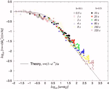
result is plotted in the scaled form 具关⌬hn共t,t0兲2兴典t₀/ At as a

function of u =␻nt in Fig. 6. Note that each curve actually

corresponds to fixed t and variable n. The fact that t varies by more than two orders of magnitude thus gives a five order of magnitude variation in u.

FIG. 6. 共Color online兲 Power spectrum of the fluctuations: scal-ing of the autocorrelation function in time and space.

(10)

Both experiments at all probed times show a fluctuation spectrum consistent with the theoretical prediction of Eq. 共52兲, which is shown as a continuous line. The initial flat

plateau corresponds first to the normal diffusion regime where f共u兲⬃1, and then the progressive saturation of the modes is seen as the straight line of slope −1 on the right-hand side, i.e., a power-law decay with f共u兲⬃1/u.

Note that the knowledge of the spatial power spectrum 具⌬˜hn

2_{典 and the equilibrium average 具h} n

2_{典 given in Eq. 共}

19兲

allows us also to evaluate the two-point correlation function in space and time. This function is defined as

G共x,t兲 = 具h共0,0兲h共x,t兲典, 共53兲 which has the spatial Fourier transform

Gn共t兲 = 具hn共0兲hn共t兲典. 共54兲

By definition of⌬hn共t兲 with t0= 0 we can write

具⌬hn共t兲2典 = 具hn共t兲2典 − 2具hn共t兲hn共0兲典 + 具hn共0兲2典, 共55兲

where the first and last right-hand-side terms are the same equilibrium averages.

Solving for Gn共t兲 above we immediately get

Gn共t兲 = 具hn2典 − 具⌬hn共t兲2典 2 = kBT

冉

1 ␻nt −1 − e −2␻nt ␻n

冊

=e −2␻nt ␻n kBT, 共56兲

where we have used Eq. 共51兲 with t0= 0 to substitute for

具⌬hn共t兲2典.

VII. THE MEMORY OF THE BROWNIAN WORM

In this section, we will show that the W⬃t1/4_{regime can}

also be understood in terms of anomalous diffusion in a sys-tem with memory. We will show how the Markovian tion for the entire chain becomes a non-Markovian descrip-tion when it is formulated for a single particle in the chain.

For such a particle linked to a background constituted of both the solvent and the rest of the chain, the motion is governed by an exterior with long-time memory in the fluc-tuating force as well as the response function.

The single particle description takes the form of a gener-alized Langevin equation of the Mori-Lee form关8兴:

mh¨0共t兲 = − m

冕

−⬁

t

dt1⌫共t − t1兲h˙0共t1兲 + F共t兲, 共57兲

with⌫共t兲 a linear response function, and F共t兲 a fluctuating function satisfying the fluctuation dissipation theorem,

具F共t兲F共0兲典 = mkBT⌫共t兲. 共58兲

From the theory of anomalous diffusion in such systems with memory, the anomalous diffusion exponent is related to the asymptotic behavior of the linear response function关8兴.

When the Laplace transform of the response function be-haves as ⌫ˆ共␻兲⬃␻−␣ when ␻→0, this theory predicts an

anomalous diffusion W2_⬃t1−␣_{. We will show that this}

sys-tem indeed follows this theoretical prediction, i.e., that it can be described by an Eq. 共57兲 with the asymptotic behavior

⌫ˆ共␻兲⬃␻−1/2_{. In other words, this alternative description also}

produces the prediction W⬃t1/4, in agreement with the direct treatment above.

A. Generalized Langevin equation for a particle in a Brownian worm

We consider a set of N particles in an immobile solvent. The inertial terms are neglected for every particle. However, for technical purposes we shall take the particle in focus to have a mass initially. This is done to exhibit a known struc-ture of the Langevin equation: eventually, the mass of this particle will also be send to zero.

Thus, we write for every particle j,

␦j0mh¨j= −␬h˙j+␣共hj+1− 2hj+ hj−1兲 +␨j, 共59兲

where␬= 3␲␩a and ␣ is the curvature of the magnetic en-ergy with respect to lateral bending, and ␨j is the

uncorre-lated Brownian force with a magnitude which is given by dissipation fluctuation theorem

具␨i共0兲␨j共t兲典 = 2␬kBT␦ij␦共t兲. 共60兲

We Fourier transform this in space fn

⬘

=

兺

j=1 N fje−2␲jn/N, fj= 1 N

兺

_n=0 N−1 fn

⬘

e2␲jn/N. 共61兲

From here on primes refer to Fourier modes in space, and tildes to Fourier modes in time to simplify notation. We then obtain − mh¨₀=␬共h˙n

⬘

+␻nhn

⬘兲 −

␨n

⬘

=␬e−␻n td dt关hn

⬘共t兲e

␻nt兴 −␨ n

⬘

, 共62兲 where ␻n= 2␣ ␬

冋

1 − cos

冉

2␲n N

冊

册

, 共63兲 i.e., when nⰆ N, ␻n⯝␻1n2, 共64兲 where ␻1= ␣ ␬ 共2␲兲2 N2 . 共65兲 Equation共62兲 is integrated as − hn

⬘共t兲 =

−⬁ ⬁ dt1mh¨0共t1兲

兺

n ␦共t − t1兲 − ⌰共t − t1兲␻ne−␻n共t−t1兲 ␬N = − h˙0共t兲 +

␻兲G˜ n共␻兲/deG共␻兲. 共73兲

An inverse Fourier transform, then leads to mh¨0共t兲 = − m

冕

−⬁ t

dt1⌫共t − t1兲h˙0共t1兲 + F共t兲共74兲

which is exactly the Mori-Lee generalized Langevin equa-tion关8兴. To replace the +⬁ upper bound of the integral by t,

we have used that the response function is causal, i.e., that ⌫共t兲=0 when t⬍0: This is shown explicitly in Appendix A. The fact that the generalized fluctuation dissipation theorem is satisfied, i.e., that

具F共t兲F共0兲典 = mkBT⌫共t兲 共75兲

is verified in Appendix B.

B. Derivation of long time behavior of the linear response function

From Eq.共68兲 and Bracewell 关39兴 we get immediately G ˜ n共␻兲 = 1 ␬N

冉

1 − ␻n ␻n+ i␻

冊

= i␻ ␬N共␻n+ i␻兲共76兲 and we need to evaluate the discrete sum

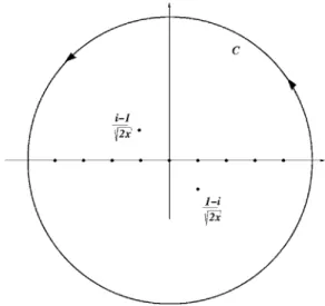
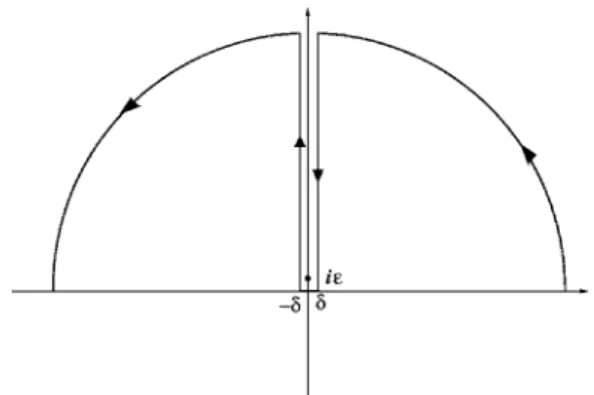
. 共81兲

To proceed, note that兰Ccotan共␲z兲f共z兲=0 for a contour C

corresponding to Rei␪ _{with R a constant that will be sent to}

infinity and␪苸关0,2␲关共cf. Fig.7兲, then by the residue

theo-rem

FIG. 7. Contour for integration of the G function in the complex plane.

(12)

_␻_/_␻ 1兲共84兲 with g共z兲 = 1 + z cotan共z兲. 共85兲 The function g共z兲 is monotonously growing, with limits g共z兲→1 when z→0, and g共z兲→␲z / 2 when z→⬁.

Consequently, for finite chains, the long time limit is given by G˜ 共␻→0兲⬃1/共2␬N兲, if␻1is fixed and finite. This

corresponds to a normal diffusive behavior.

However, for very long chains, the transient time to reach this saturaton is extremely long, and corresponds to the re-gime physically probed by the system. This is seen by taking first the N→⬁ limit in the above, so that using ␻2=␻1N1

=共2␲兲2_␣_/_␬_, G ˜ 共␻兲 =␲2i3/2 4␬N

冑

␻/␻1= ␲2_i3/2 4␬

冑

␻/␻2= ␲i3/2 8

冑

␻/共␣␬兲共86兲 for any␻.

Thus, the Fourier transform of the response function is from Eq.共72兲, ⌫˜共␻兲 = 2␬ ␲m

冑

␻2 i␻= 4 m

冑

␣␬ i␻, 共87兲

and from Ref.关8兴, since the Laplace transform ⌫ˆ of ⌫ in the

limit of small␻共long times兲 behaves as

⌫ˆ共␻兲 ⬃ ⌫˜共− i␻兲 ⬃␻−1/2_, _共88兲

we have for the rms displacement of the observed particle, 具x2_{共t兲典 ⬀ t}1−1/2_{= t}1/2 _共89兲

which is nothing but the subdiffusive regime we observe up until saturation. Thus, our system experimentally, analyti-cally, and numerically verifies the theory for anomalous dif-fusion in systems with memory derived in Ref.关8兴, and thus

provides an experimental realization of this theory.

VIII. CONCLUSION

Chains of dipoles suspended between two plates, roughen dynamically under the effect of thermal disorder when the dipolar interaction is decreased. This dynamic roughening is intimately related to the scaling of the equilibrium

fluctua-tion of these chains. We have studied the dynamic roughen-ing experimentally and theoretically and the equilibrium fluctuations of such chains composed of magnetic holes in a ferrofluid. Their dynamic roughening and fluctuations are shown to behave according to a discrete Rouse model. The rms width of these chains behaves initially as normal diffu-sion, W2_{⬀t, then it grows with an anomalous exponent, i.e.,}

W2⬀t1/2 as Fourier modes progressively saturate from the small scales to the large ones. Eventually W reaches an am-plitude W2_{⬃N at large times. We have derived this behavior}

analytically, including the prefactors, and verified that the experimental data coincide with the theoretical predictions over five decades in the case of the equilibrium fluctuations. The analytic predictions and experiments also coincide with Brownian dynamic simulations taking into account the non-linearities of the interaction potential, and the interactions beyond nearest neighbors.

Eventually, we have shown that the Markovian descrip-tion of the entire Brownian worm can be reduced to a non-Markovian one for a single particle. This description con-tains a linear response function, with a long time tail decaying as t−␣with␣= 1 / 2. Thus, since these chains experi-mentally exhibit the anomalous diffusion exponent 1 / 2 = 1 −␣, predicted by the theory of diffusion in systems with memory, they constitute a first experimental realization of this theory.

APPENDIX A: DERIVATION OF THE REAL-TIME EXPRESSION OF THE RESPONSE FUNCTION

We will now perform the inverse time Fourier transform 共TFT兲 from Eq. 共87兲: for that purpose, we introduce a small

i +␦=1+i_冑

2, and lim␦→0+

冑

i −␦= −1−i

冑₂ .

For t⬍0, we close the contour in complex plane by a half-circle in the lower half-plane, and since no singularity is enclosed,⌫共t兲=0 in that case: the response function is causal as desired.

冑

␻2

m

冑

␲3t=⌰共t兲 4

冑

␬␣

(13)

APPENDIX B: AUTOCORRELATION FUNCTION OF THE FLUCTUATING FORCE

We will here check directly the validity generalized fluc-tuation dissipation theorem for our specific system with memory, i.e., derive Eq.共75兲.

We will first use the fluctuation dissipation theorem on the basic set of equations, that led to Eq.共60兲 for the

autocorre-lation function of the fluctuating force from the fluid on ev-ery particle. Performing a space Fourier transform, Eq.共60兲

translates for the correlations between the Fourier modes of the fluctuating force, to

具␨m

⬘

共t兲␨n

⬘

*共0兲典 = 2NkBT␦mn␦共t兲. 共B1兲

We now perform a TFT of␨_n

⬘共t兲 to obtain from the above and

Eq.共70兲, 具˜␨ m

⬘

共␻兲˜␨ n

⬘

*_共_␻

_{⬘兲典 =}

冊

1/2 共B5兲共see Fig.9for the contour adopted in application of the resi-due theorem兲. Thus, introducing the notation

具F共t兲F*_{共0兲典 = g共t兲} _共B6兲

we obtain from Eqs.共87兲 and 共B4兲–共B6兲, g

˜共␻兲 =8␬kBT ␲

冑

2

冑

␻1

␻ = 2mkBT关⌫˜共␻兲 + ⌫˜*共␻兲兴共B7兲

which means that

具F共t兲F*_{共0兲典 = 2mk}

BT⌫共兩t兩兲, 共B8兲

where we have used the fact that since the response function is real, ⌫˜*_共_␻_{兲 =} 1 2␲

冕

−⬁ ⬁ ⌫共t兲ei␻t dt = 1 2␲

冕

−⬁ ⬁ ⌫共− t兲e−i␻t_dt _共B9兲

and since it is causal,⌫共t兲+⌫共−t兲=⌫共兩t兩兲. Equation 共B8兲

cor-responds to the fluctuation dissipation theorem for a system with memory, as presented in Ref.关8兴.

FIG. 8. Contour for the obtention of the linear response func-tion, in the complex plane.

FIG. 9. Contour in the complex plane for the integration of the time autocorrelation of the fluctuating force.

(14)

关1兴 A. T. Skjeltorp, Phys. Rev. Lett. 51, 2306 共1983兲.

关2兴 R. Toussaint, J. Akselvoll, G. Helgesen, A. T. Skjeltorp, and E. G. Flekkøy, Phys. Rev. E 69, 011407共2004兲.

关3兴 A. Skjeltorp and G. Helgesen, Physica A 176, 37 共1991兲. 关4兴 J. Ugelstad and P. Mork, Adv. Colloid Interface Sci. 13, 101

共1980兲.

关5兴 R. Toussaint, G. Helgesen, and E. G. Flekkøy, Phys. Rev. Lett.

93, 108304共2004兲.

关6兴 A. Y. Grosberg and A. R. Khokhlov, Statistical Physics of Macromolecules共AIP Press, New York, 1994兲.

关7兴 S. F. Edwards and D. R. Wilkinson, Proc. R. Soc. London, Ser. A 381, 17共1982兲.

关8兴 R. Morgado, F. A. Oliveira, G. G. Batrouni, and A. Hansen, Phys. Rev. Lett. 89, 100601共2002兲.

关9兴 E. M. Furst and A. P. Gast, Phys. Rev. E 62, 6916 共2000兲. 关10兴 E. M. Furst and A. P. Gast, Phys. Rev. E 58, 3372 共1998兲. 关11兴 S. Cutillas and J. Liu, Phys. Rev. E 64, 011506 共2001兲. 关12兴 A. S. Silva, R. Bond, F. Plouraboué, and D. Wirtz, Phys. Rev.

E 54, 5502共1996兲.

关13兴 M. R. Jolly, J. W. Bender, and J. D. Carlson, J. Intell. Mater. Syst. Struct. 10, 5共1999兲.

关14兴 S. F. Dyke, B. F. Spencer, M. K. Sain, and J. D. Carlson, Smart Mater. Struct. 7, 693共1998兲.

关15兴 Proceedings of the 5th International Conference on Electro-rheological Fluids, Magneto-Electro-rheological Suspensions and Associated Technology, edited by W. A. Bullough共World Sci-entific, Singapore, 1996兲.

关16兴 O. Ashour, C. Rogers, and W. Kordonsky, J. Intell. Mater. Syst. Struct. 7, 123共1996兲.

关17兴 J. A. Stangroom, Phys. Technol. 14, 290 共1983兲.

关18兴 T. C. Halsey and W. Toor, J. Stat. Phys. 61, 1257 共1990兲. 关19兴 T. C. Halsey and W. Toor, Phys. Rev. Lett. 65, 2820 共1990兲. 关20兴 T. C. Halsey, J. Colloid Interface Sci. 156, 335 共1993兲. 关21兴 J. E. Martin, J. Odinek, and T. C. Halsey, Phys. Rev. Lett. 69,

1524共1992兲.

关22兴 J. E. Martin, K. M. Hill, and C. P. Tigges, Phys. Rev. E 59,

5676共1999兲.

关23兴 M. Fermigier and A. P. Gast, J. Colloid Interface Sci. 154, 522 共1992兲.

关24兴 G. Helgesen, A. T. Skjeltorp, P. M. Mors, R. Botet, and R. Jullien, Phys. Rev. Lett. 61, 1736共1988兲.

关25兴 S. Fraden, A. J. Hurd, and R. B. Meyer, Phys. Rev. Lett. 63, 2373共1989兲.

关26兴 J. E. Martin, J. Odinek, T. C. Halsey, and R. Kamien, Phys. Rev. E 57, 756共1998兲.

关27兴 J. Liu, E. M. Lawrence, A. Wu, M. L. Ivey, G. A. Flores, K. Javier, J. Bibette, and J. Richard, Phys. Rev. Lett. 74, 2828 共1995兲.

关28兴 J. Cernak, G. Helgesen, and A. T. Skjeltorp, Phys. Rev. E 70, 031504共2004兲.

关29兴 Type EMG 909, produced by Ferrofluidics Corporation, 40 Simon St., Nashua, NH 03061.

关30兴 B. Bleaney and B. Bleaney, Electricity and Magnetism 共Ox-ford University Press, Ox共Ox-ford, 1978兲.

关31兴 P. G. De Gennes and P. Pincus, Phys. Kondens. Mater. 11, 1970共1970兲.

关32兴 E. G. Flekkøy and D. H. Rothman, Phys. Rev. E 53, 1622 共1996兲.

关33兴 E. G. Flekkøy and D. H. Rothman, Phys. Rev. Lett. 75, 260 共1995兲.

关34兴 F. Reif, Fundamentals of Statistical and Thermal Physics 共McGraw-Hill, Singapore, 1965兲.

关35兴 F. Family and T. Vicsek, J. Phys. A 18, L75 共1985兲.

关36兴 L. P. Faucheux and A. J. Libchaber, Phys. Rev. E 49, 5158 共1994兲.

关37兴 M. Sahimi, Flow and Transport in Porous Media and Frac-tured Rocks共Wiley-VCH, New York, 1995兲.

关38兴 W. H. Press et al., Numerical Recipes 共Cambridge University Press, New York, 1992兲.

关39兴 R. N. Bracewell, The Fourier Tranform and its Applications, 3rd ed.共McGraw-Hill, Singapore, 2000兲.