Heat flow density estimates in the Upper
Rhine Graben using laboratory measurements
of thermal conductivity on sedimentary rocks
Pauline Harlé
1*, Alexandra R. L. Kushnir
2, Coralie Aichholzer
1, Michael J. Heap
2, Régis Hehn
3, Vincent Maurer
3,
Patrick Baud
2, Alexandre Richard
3, Albert Genter
3and Philippe Duringer
1Abstract
The Upper Rhine Graben (URG) has been extensively studied for geothermal exploita-tion over the past decades. Yet, the thermal conductivity of the sedimentary cover is still poorly constrained, limiting our ability to provide robust heat flow density esti-mates. To improve our understanding of heat flow density in the URG, we present a new large thermal conductivity database for sedimentary rocks collected at outcrops in the area including measurements on (1) dry rocks at ambient temperature (dry); (2) dry rocks at high temperature (hot) and (3) water-saturated rocks at ambient tem-perature (wet). These measurements, covering the various lithologies composing the sedimentary sequence, are associated with equilibrium-temperature profiles measured in the Soultz-sous-Forêts wells and in the GRT-1 borehole (Rittershoffen) (all in France). Heat flow density values considering the various experimental thermal conductivity conditions were obtained for different depth intervals in the wells along with average values for the whole boreholes. The results agree with the previous heat flow density estimates based on dry rocks but more importantly highlight that accounting for the effect of temperature and water saturation of the formations is crucial to providing accurate heat flow density estimates in a sedimentary basin. For Soultz-sous-Forêts, we calculate average conductive heat flow density to be 127 mW/m2 when considering hot rocks and 184 mW/m2 for wet rocks. Heat flow density in the GRT-1 well is esti-mated at 109 and 164 mW/m2 for hot and wet rocks, respectively. Results from the Rit-tershoffen well suggest that heat flow density is nearly constant with depth, contrary to the observations for the Soultz-sous-Forêts site. Our results show a positive heat flow density anomaly in the Jurassic formations, which could be explained by a combined effect of a higher radiogenic heat production in the Jurassic sediments and thermal disturbance caused by the presence of the major faults close to the Soultz-sous-Forêts geothermal site. Although additional data are required to improve these estimates and our understanding of the thermal processes, we consider the heat flow densities estimated herein as the most reliable currently available for the URG.
Keywords: Heat flow density, Upper Rhine Graben, Thermal conductivity, Saturation,
Temperature, Sedimentary rocks, Geothermal energy, Soultz-sous-Forêts, Rittershoffen
Open Access
© The Author(s) 2019. This article is licensed under a Creative Commons Attribution 4.0 International License, which permits use, sharing, adaptation, distribution and reproduction in any medium or format, as long as you give appropriate credit to the original author(s) and the source, provide a link to the Creative Commons licence, and indicate if changes were made.The images or other third party material in this article are included in the article’s Creative Commons licence, unless indicated otherwise in a credit line to the material. If material is not included in the article’s Creative Commons licence and your intended use is not permitted by statutory regulation or exceeds the permit-ted use, you will need to obtain permission directly from the copyright holder.To view a copy of this licence, visit http://creativecommons. org/licenses/by/4.0/.
RESEARCH
*Correspondence: [email protected] 1 Institut de Physique du Globe de Strasbourg (IPGS), UMR 7516, CNRS-Université de Strasbourg EOST, 1 Rue Blessig, 67084 Strasbourg Cedex, France
Full list of author information is available at the end of the article
Background
The Upper Rhine Graben (URG) has been known to be a region of high heat flow density for more than 40 years (Cermák and Rybach 2012; Gable 1986; Lucazeau and Vasseur 1989; Rybach 2007; Vasseur 1980, 1982). This regional conductive heat flow density anomaly is due to crustal thinning caused by extension during the Cenozoic and facilitated by the basin-wide deep-rooted groundwater circulation that locally enhances the surface heat flow density (Clauser and Villinger 1990; Schellschmidt and Schulz 1992). Due to the heat flow density anomaly, the URG represents an ideal region for geothermal exploitation. Located in the northeastern part of France and southwestern part of Germany (Fig. 1), this continental rift is already home to several operational (e.g., Soultz-sous-Forêts and Rittershoffen, both France, and Bruchsal, Insheim and Landau, all in Germany) and planned (e.g., Illkirch, Vendenheim, and Wissembourg, all France) geothermal sites (Aichholzer et al. 2016; Vidal and Gen-ter 2018), but accurate estimates of heat flow density remain crucial for temperature estimations prior to drilling operations and thermodynamic models that inform our understanding of measured temperature profiles for continued geothermal explora-tion (Beardsmore et al. 2001; Flores Marquez 1992; Frone et al. 2015; Schütz et al. 2014).
Thermal profiles of operational wells have revealed conductive heat flow density in the upper 1–1.5 km, as opposed to convective heat flow density common to the geo-thermal reservoir (Bächler et al. 2003; Baillieux et al. 2013; Clauser and Villinger 1990; Guillou-Frottier et al. 2013; Kohl et al. 2000; Le Carlier et al. 1994; Magnenet et al. 2014; Pribnow and Schellschmidt 2000). When conductive regime dominates in the Earth’s crust, conductive heat flow density (also called surface or terrestrial heat flow density) is estimated using Fourier’s law of heat conduction q = × T
z , where q is the conductive heat flow density (W/m2), λ is thermal conductivity (W/mK) and
T z is the temperature gradient (°C/m) (Beardsmore et al. 2001). Conductive heat flow density can thus be defined as the product of the thermal gradient and the mean ther-mal conductivity of the medium. Therther-mal conductivity describes the capacity of a material to transfer heat in the presence of a thermal gradient and is a major parame-ter controlling the conductive heat flow density. The thermal conductivity of the rocks depends not only on mineralogical composition and microstructure (porosity, frac-ture density, texfrac-ture), but also on pressure, rock temperafrac-ture and degree of saturation and nature of the fluid. The effect of those parameters on thermal conductivity have been largely investigated by previous studies, which showed that the thermal conduc-tivity of rocks generally decreases with increasing porosity (Woodside and Messmer 1961; Popov et al. 2003; Nagaraju and Roy 2014; Guo et al. 2017; Mielke et al. 2017), whereas pressure tends to reduce porosity, close (micro)cracks and improve heat transport at grain–grain contacts and, thus, increase thermal conductivity (Walsh and Decker 1966; Abdulagatova et al. 2009; Schön and Dasgupta 2015). On the con-trary, high temperature tends to decrease the thermal conductivity of rocks due to differential thermal expansion of the minerals, which may increase contact resist-ances between the grains and result in thermal cracking creating porosity (Vosteen
and Schellschmidt 2003; Abdulagatov et al. 2006; Abdulagatova et al. 2009; Guo et al. 2017). Finally, thermal conductivity increases with water saturation compared to dry conditions as water conducts heat much better than air (Zimmerman 1989; Popov et al. 2003; Schütz et al. 2012; Nagaraju and Roy 2014; Guo et al. 2017; Albert et al. 2017).
Thus, at prospective geothermal sites where conduction dominates heat transfer in the upper few kilometers of the crust, a combined understanding of the geology and the thermal conductivity of the rocks (preferably at the in situ temperature and fluid satura-tion condisatura-tions) can be used to provide useful conductive heat flow density estimates.
Studies have defined a mean conductive heat flow density between 100 and 120 mW/ m2 in the URG, with a maximum value of 150 mW/m2 at Soultz-sous-Forêts (Baillieux et al. 2013; Kohl et al. 2000), much higher than the mean value of 60 mW/m2 in Europe (Majorowicz and Wybraniec 2011). Unfortunately, the absence of a large database for thermal conductivities of sedimentary rocks from the region implies that these heat flow density estimates are based on a limited number of thermal conductivity values, often determined for general lithologies that may not be fully representative of the formations within the graben (Flores Marquez 1992). This lack of data for the upper part of the sedi-mentary cover can lead to unreliable estimations of the local heat flow density (Fuchs and Balling 2016). Moreover, the thermal conductivity values considered for these early heat flow density estimations are for rocks in the dry state at ambient temperature and the absence of URG-specific models makes them difficult to port to in situ conditions. Indeed, while mixing models (Abdulagatova et al. 2009; Fuchs et al. 2013; Vosteen and Schellschmidt 2003) are valuable when no or very few samples from the study area are available, it is always preferable to gather a regional database when possible. Thus, new thermal conductivity measurements under various temperature and saturation condi-tions for a wide range of sedimentary formacondi-tions from the URG are required to provide robust heat flow density estimates.
Although geothermal exploitation is well-developed in the URG, the thermal conduc-tivity of the sedimentary cover is still poorly known, mostly due to the lack of core mate-rial, in particular in the upper strata (above the Muschelkalk series) where conduction predominates.
Here, we analyze the behavior of thermal conductivity of sedimentary rocks sampled in the URG as a function of different parameters including porosity, fluid saturation and temperature, with the aim of providing a new thermal conductivity database for the URG. This large database is used to provide more accurate heat flow density estimates for sites where an equilibrium-temperature profile is known. The influence of the vari-ous thermal conductivity measurement conditions on the calculated heat flow density is also investigated. Using these laboratory data, we estimate the heat flow density for the Soultz-sous-Forêts and Rittershoffen operational industrial wells.
The geology of the Upper Rhine Graben (URG)
To perform this study, we collected analogue rock samples that best represent the geo-logical formations of the Upper Rhine Graben.
In this study, “facies” refers to the lithology (rock type), sedimentary structures and depositional environments characterizing the rock. “Sedimentary formation” refers to a set of homogenous sedimentary strata with the same facies and paleontological content and characterized by obvious lower and upper boundaries. A “series” of formations, like the Muschelkalk or the Buntsandstein series, refers to a group of sedimentary formations deposited within the same geodynamic context, for example in fluvial systems for the
Buntsandstein.
In the URG, the deep Paleozoic basement is covered by Permian clastic forma-tions. Above these Permian sedimentary rocks are the fluvial to fluvio-deltaic sand-stones and conglomerates of the lower Triassic Buntsandstein (B) series, overlain by
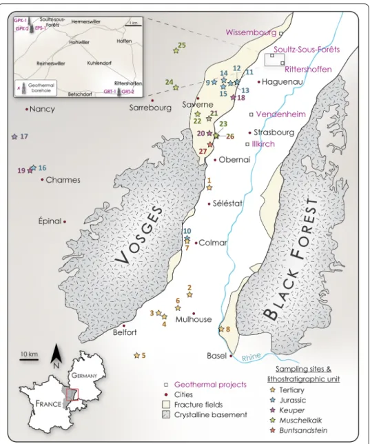
Fig. 1 Map of the Upper Rhine Graben showing the sampling sites and the existing and prospective
geothermal projects. Numbered stars refer to sampling locations, given in Figs. 2 and 3. The color of the stars indicates the lithostratigraphic unit. More than one lithostratigraphic unit was sampled in locations 17, 21 and 26 (modified after Aichholzer et al. (2016))
marine-to-lagoonal sediments of the middle Triassic Muschelkalk (M) series (Aichholzer et al. 2016). The Muschelkalk formations are mainly composed of interbedded marly-calcareous rocks, shelly sandstones, evaporitic deposits, and dolostones (Duringer et al. 2019; Ménillet 2015). The carbonate-shelf environment that formed the upper
Muschel-kalk series was followed by the evaporitic episode of the Keuper (K), upper Triassic. The Keuper is characterized by massive clays, marly clays and dolomites that contain
evapor-itic deposits (gypsum and anhydrite). Some sandstone marker beds are also encountered in the lower, middle and upper Keuper formations (Aichholzer et al. 2016; Duringer et al. 2019; Ménillet 2015). The depositional environment became fully marine from the Juras-sic, with marls/limestones alternations during Hettangian, followed by clays and clayey marls alternations with occasional calcareous banks up to the base of Bajocian. Bajocian was characterized by carbonate-shelf episodes (Duringer et al. 2019; Ménillet 2015). The sedimentary formations described above were deposited before the rift episode of the graben and can be found beyond the borders of the URG.
The Tertiary rocks were unconformingly deposited on top of the eroded upper Juras-sic sediments (Berger et al. 2005; Duringer et al. 2019; Hinsken et al. 2007, 2011; Roussé 2006; Sittler 1965, 1992). Eocene and lower Oligocene formations are composed, from base to top, by lacustrine and evaporitic clays, marls, limestones and a few sandstones in the central part of the graben and conglomerates on the borders (Zone Dolomitique,
Couche Rouge and Couches de Pechelbronn in the North and Zone Salifère inférieure, moyenne and supérieure in the South (see Duringer et al. 2019). Middle and upper Oligocene deposits are formed by marine clays and marls intercepted by some poorly cemented sandstones (Série Grise). The retreat of the sea in the graben at the end of the Rupelian (upper Oligocene) led to the deposition of the thick formation of the Couches
de Niederroedern also called Série Bariolée. This formation is a lacustrine-to-fluvial
var-iegated marly formation attributed to the Chattian (Berger et al. 2005; Hinsken et al. 2007, 2011; Roussé 2006; Sittler 1965). The upper Oligocene is eroded in some parts of the rift and the Miocene does not exist in the whole graben due to erosion (Aichholzer et al. 2016; Berger et al. 2005; Roussé 2006). The uppermost part of the sedimentary cover is characterized by a continental episode made of fluvial to ephemeral lake depos-its that were formed during the Pliocene. Loess deposited during the Quaternary ends the sedimentary cover (Duringer et al. 2019; Ménillet 2015).
Case study: the Soultz‑sous‑Forêts geothermal site
Started in the 1980s, the Soultz-sous-Forêts (northern Alsace, France) (Fig. 1) project was the first Enhanced Geothermal System (EGS) developed in the world (Baria et al. 1999; Genter et al. 2010; Gérard et al. 2006; Kappelmeyer 1991). The geology at the Soultz-sous-Forêts site is well known thanks to an old exploratory oil borehole, EPS-1, that was deepened for the needs of geothermal exploration and fully cored from 933 (middle Muschelkalk) to 2227 m (Paleozoic basement) (Aichholzer et al. 2019; Dezayes et al. 2005) e.g., in the zone where convection predominates (Genter and Traineau 1992). The Permian and Triassic sedimentary rocks of the Buntsandstein are described in Aich-holzer et al. (2016, 2019) and Vidal et al. (2015) and physical properties of the EPS-1 cores studied by Géraud et al. (2010), Griffiths et al. (2016), Haffen (2012), Haffen et al. (2013, 2017), Heap et al. (2017, 2018, 2019), Kushnir et al. (2018), Surma and Geraud
(2003), Schellschmidt and Clauser (1996), Flores Marquez 1992 and Schellschmidt and Schulz (1992).
In total, four boreholes have been drilled at the Soultz-sous-Forêts site: GPK-1, GPK-2, GPK-3, and GPK-4, the last three of which extend to a depth of 5 km. The stratigraphy of the GPK-1 and 2 boreholes was described in detail by Aichholzer et al. (2016) and is composed of 1400 m (measured depth, MD) of sedimentary cover. These boreholes have provided precious data including temperature profiles that inform on regional heat transfer mechanisms (conduction and convection). At Soultz-sous-Forêts, the typical equilibrium-temperature profiles measured in the 5-km-deep wells revealed a tempera-ture of 200 °C at a depth of 5 km. Importantly, the temperatempera-ture profile can be divided into three parts (Genter et al. 2010, 2015; Vidal et al. 2015). First, the uppermost part of the well (between 0 and 1 km-depth, down to the top of the Muschelkalk series), composed of sedimentary formations (Tertiary, Jurassic, and Upper Triassic), features a geothermal gradient of 110 °C/km, which, in the URG, indicates a conductive regime (Pribnow and Schellschmidt 2000). The section between a depth of 1 and 3.5 km, com-prising the sedimentary rocks of the Buntsandstein series (down to a depth of about 1400 m) and fractured granitic basement, is characterized by a very low thermal gradient of 5 °C/km, interpreted as convective regime in the URG. Finally, the deepest part of the thermal profile, below a depth of 3.5 km, is composed exclusively of crystalline basement and features a thermal gradient of 30 °C/km, indicating another conduction zone. At the Soultz-sous-Forêts site, the previously estimated heat flow densities range between 140 and 150 mW/m2 (Baillieux et al. 2013; Flores Marquez 1992; Pribnow and Clauser 2000; Le Carlier et al. 1994; Schellschmidt and Clauser 1996).
Case study: the Rittershoffen geothermal site (France)
The Rittershoffen geothermal site, located 6 km southeast of Soultz-sous-Forêts (Fig. 1), is the second EGS project developed in northern Alsace (Baujard et al. 2017). To date, no heat flow density has been calculated for the Rittershoffen geothermal site. However, a heat flow density of 121 mW/m2 has been calculated for a nearby borehole (SAN 1 (SANDMUHLE 1) borehole, about 3.5 km from the GRT-1 well) (Lucazeau 2019). The drilled GRT-1 and GRT-2 boreholes extend to a depth of 2580 and 3196 m MD, respec-tively, and target the geothermal reservoir located at the sediment–basement inter-face. Temperature measurements in the wells indicate a constant thermal gradient of 87 °C/km (conduction) in the sedimentary cover between the surface and the top of the
Muschelkalk (1661 m depth MD), and an average temperature of 160 °C at the top of
the Muschelkalk cap rock (Baujard et al. 2017). The very low gradient (3° C/km) below this depth threshold indicates a convective regime in the Muschelkalk and Buntsandstein sedimentary formations, and in the fractured granitic basement.
Stratigraphy of the 2200-m-thick sedimentary cover in GRT-1 has been recently updated by Duringer et al. (2019) and correlated with stratigraphy in GPK-1 and GPK-2 in Aichholzer et al. (2016), which revealed several variations in the sedimentary cover between the two sites and even between the two wells at Soultz-sous-Forêts. Differences include missing layers due to erosion, lateral thickness variations in sedimentary forma-tions and thinning or absence of some formaforma-tions due to faulting.
Methods
Selecting representative rock samples
We collected 45 samples (typically 15 × 15 × 15 cm) from 27 different locations in the east of France (Alsace, Lorraine and Franche-Comté) and in Southwest Germany (Baden-Württemberg) (Figs. 1, 2, 3) that we consider provide a representative suite of rocks for the sedimentary cover of the URG. The choice of samples collected was guided by the formations encountered in the wells at Rittershoffen (Duringer et al. 2019) and the wells at Soultz-sous-Forêts (Aichholzer et al. 2016). But for completeness, we sam-pled additional formations that are widespread in the region including, for instance, the
Grande Oolithe [J-GO (Fig. 2)] formation, which is absent in the northern part of the URG due to erosion, but encountered to the south of Haguenau. We did not only sample the thickest formations, but also formations that represent outliers, in terms of lithology and texture, that may be characterized by very different thermal conductivities. Most samples were collected from rock outcrops, those not available at outcrops were col-lected at the potash mines in Wittelsheim (France) (O-ZSS samples) or sourced from drill cores from the DP202 borehole in Pulversheim (France) (O-CN and O-CM sam-ples). We note that poorly consolidated formations were not sampled because it was not possible to prepare a sample suitable for measurement in the laboratory. The sampled
Fig. 2 List of Tertiary and Jurassic samples classed in stratigraphic order. Lithostratigraphic unit, number
of the sampling site (see Fig. 1 for location on the map), nature of the sampled rock and location of the sampling site are indicated
formations that most closely represent those that could not be sampled were used as proxies.
Our method to estimate heat flow density is designed to be used at prospective geo-thermal sites for which there are no boreholes, therefore, in the absence of site-specific rock samples. Although measurements on analogue samples should be used with care (Bauer et al. 2017), we have chosen to measure samples taken from rock outcrops for several reasons. First, when boreholes do exist (such as at Soultz-sous-Forêts and Rit-tershoffen), the recovered rock cuttings are often too small to make reliable laboratory measurements. Further, despite having cores from exploration well EPS-1 (at the Soultz-sous-Forêts site), these cores are only available from a depth of 933 m and therefore do not sample the conduction zone. Finally, not all regionally significant formations are encountered in the boreholes at Rittershoffen and Soultz-sous-Forêts (e.g., such as the
Grande Oolithe, J-GO). Therefore, the accurate estimation of heat flow density is reliant
on the establishment of a comprehensive thermal conductivity database developed using analogue geological materials that are representative of the local and regional geology, including outcrop material.
Sample preparation
Each rock sample was cut and polished to obtain two planer and parallel surfaces (Fig. 4a). When possible, two pieces of sample for each studied formation were prepared. The thickness of the prepared samples was typically between 2.5 and 4 cm to allow a probing depth sufficient for the measurement and so that the samples could fit in the experimental jig (Fig. 4b, c). As a precaution, samples considered sensitive to water, such as the potash and marls, were cut and polished without using water to minimize water– mineral reactions that could affect the physical state of the samples.
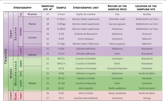
Fig. 3 List of Keuper, Muschelkalk and Buntsandstein samples classed in stratigraphic order. Lithostratigraphic
unit, number of the sampling site (see Fig. 1 for location on the map), nature of the sampled rock and location of the sampling site are indicated
Before characterization, all samples were vacuum-dried at 40 °C overnight.
Porosity measurements
The connected porosity of the samples was measured to inform on the relationship between thermal conductivity and porosity. We used the triple-weight water satura-tion method (Guéguen and Palciauskas 1992). The dry samples were vacuum-satu-rated with water and the satuvacuum-satu-rated mass (mw) and the immersed saturated mass (mi) of the samples were measured. The samples were then vacuum-dried again and the dry mass (md) of each sample was measured. The connected water porosity, φ , was calculated using the following equation (units: unitless, value given as %):
The porosities of the gypsum and the marl samples were not assessed for the sam-ples on which thermal conductivity measurements were made; a separate sample set was dedicated to porosity measurements for these rocks. Although the thermal con-ductivities of these samples were measured in the wet condition (explained below), we wanted to avoid wet–dry cycles that may have influenced the physical state of these samples prior to measuring their thermal conductivity. The porosity of the pot-ash samples could not be measured due to their dissolution upon exposure to water.
(1) φ = mw−md
mw−mi .
Fig. 4 a Example of a sample prepared for thermal conductivity measurements (sample J-CE; Calcaire
d’Ettendorf). The samples were cut and polished to produce at least two planar and parallel surfaces. b Double-sided thermal conductivity measurement on J-CE sample in the dry state at ambient temperature. The two pieces of sample are placed either side of the sensor. The pieces are clamped together, to ensure a good contact between the pieces of sample and the sensor, using a metal screw at the top of the jig. c Schematic showing the setup and the volume around the sensor (probing depth) investigated during the measurement
Thermal conductivity measurements
The thermal conductivity measurements were conducted in the laboratory using a ther-mal analyzer (model TPS 500 by Hot Disk) based on the Transient Plane Source (TPS) method with a Kapton-plastic coated sensor (Gustafsson 1991; Gustavsson and Gustafs-son 2005).
All the measurements were carried out at ambient pressure. The measurements were first conducted on oven-dry samples at room temperature (“dry”), then on water-sat-urated samples at room temperature (“wet”) and, finally, on oven-dry samples at high temperature (“hot”; up to 160 °C). Samples could not be measured in the saturated state at high temperature nor at higher pressure conditions due to equipment constraints. The dry, wet, and hot measurements were all carried out on the same suite of rock samples. Whenever bedding was visible, the measurements were conducted such that the bed-ding was parallel to the sensor. Anisotropy of the samples could not be studied since the thermal analyzer used for the measurements averages the thermal properties of the investigated volume of rock.
Dry measurements
The dry measurements were carried out first because they are quick to perform and there is no risk of damaging the rock samples. To perform a measurement, the prepared, planer surfaces of two pieces of rock sample were placed either side of the sensor and the sam-ples clamped together using a metal screw at the top of the jig, ensuring that the sample surfaces were flush with the sensor (Fig. 4b, c). During the measurement, an electrical current was passed through the sensor for a specified duration to increase sample tem-perature; the sensor recorded the temperature increase of the sample as a function of time. The Hot Disk software used these data to determine the thermal conductivity and thermal diffusivity (the specific heat capacity was calculated using these measured data). The temperature of the sample before the measurement (monitored using a hand-held thermometer) was also used in the calculation performed by the software. The measure-ment parameters (output power and measuremeasure-ment duration) depended on the thermal properties of the sample. For our measurements, we used output powers between 35 and 440 mW and measurement durations between 2.5 and 40 s. We performed four meas-urements on each set of samples using the four permutations of sample configuration (since each sample has two plane parallel faces). The measurements were performed at least 5 min apart and once the sample had cooled back to room temperature following each measurement. For some formations, only one piece of sample could be prepared. To measure these samples, we used a piece of insulating foam of known thermal properties in place of the second piece of sample; the foam has a thermal conductivity, measured using the Hot Disk Analyzer, at least 10 times lower than that of the measured sample.
Wet measurements
We performed wet measurements on at least two samples per lithology (limestone, sandstone, dolostone, gypsum, and marl). The first sample was the sample closest to the mean dry thermal conductivity for that lithology. The second was the sample with either the lowest or highest dry thermal conductivity for a given lithology, depending on the
distribution of dry conductivity for that lithology. Wet measurements on the marls could only be conducted on the K-MISm marls from the Marnes Irisées supérieures (K-MIS;
Keuper) formation (Fig. 3), which remained coherent following saturation with water. The wet measurements were performed on samples vacuum-saturated with water using the same Hot Disk method described above. To ensure the samples remained water-sat-urated during the measurement, the entire sample jig was submerged in a water-filled container. Once the measurements were complete, the samples were air-dried and then vacuum-dried in an oven at 40 °C, as described above.
Hot measurements
The hot measurements were performed last in case exposure to high temperature resulted in any changes to the rock microstructure (such as thermal microcracking) or mineral assemblage (e.g., the dehydroxylation of clays). Although the marls and gyp-sums may have been affected by exposure to water during the wet measurements, we decided to perform the measurements in the same order for consistency. Hot measure-ments were performed on the same samples as used for the wet measuremeasure-ments. Addi-tionally, the thermal conductivities of the O-ZSSpo potash and the J-MO (Fig. 2) marls, which could not be measured wet, were measured at high temperature. The hot meas-urements were performed at temperatures between 50 and 160 °C (Additional file 1). The hot measurements were performed on oven-dry samples using the same Hot Disk method described above (using a sensor designed to withstand high temperatures). To perform the measurements, the entire sample jig was placed inside an oven. The tem-perature was then increased at a heating rate of 5 °C/min until the target temtem-perature was reached. After the oven had reached the programmed temperature, the stability of the sample temperature was monitored using the dedicated function of the Hot Disk and the measurements were only performed once the sample was at thermal equilibrium with temperature in the oven. A waiting time of at least 30 min between two consecutive measurements was used for the hot measurements.
The chosen target temperatures for each lithology depended on the temperature expected for that lithology in the subsurface and based on temperatures measured in the GPK-2 (Soultz-sous-Forêts) (Genter et al. 2010) and GRT-1 (Rittershoffen) wells (Bau-jard et al. 2017). For the formations not encountered in these wells, such as the Grande
Oolithe (J-GO), the target temperatures were chosen based on the likely temperatures at
the expected depths for these formations.
Thermal conductivity results
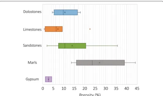
The measured thermal conductivities (“dry” for all samples and “wet” and “hot” for select samples) and connected porosities are given in Additional file 1. The connected porosity of our samples varies between 5 and 18% for the dolostones, between 0.5 and 22% for the limestones, between 2 and 36% for the sandstones, between 14 and 44% for the marls, and between 1 and 4% for the gypsum (Additional file 1; Fig. 5).
Thermal diffusivity and heat capacity of the samples are given in Additional file 1, but will not be discussed in this study.
Dry‑state samples at ambient temperature
Dry thermal conductivity is plotted as a function of porosity in Fig. 6. This figure shows that dry thermal conductivity decreases as porosity is increased. In our dataset, the range of thermal conductivity for a given porosity increased as porosity decreased. Despite the trend of decreasing thermal conductivity with increasing porosity, thermal conductivity also varies as a function of lithology. For example, the thermal conductivi-ties of sandstone, limestone, and gypsum of similar porosiconductivi-ties (ɸ ~ 2%) are ~ 4, ~ 2.5 to 3, and ~ 1.5 W/mK, respectively. For the low-porosity samples (< 20%), our results suggest
Fig. 5 Box and whisker plots of porosity ranges measured for the various lithologies
Fig. 6 Box and whisker plots of thermal conductivity ranges for the various lithologies, measurements on
samples in the dry state at ambient temperature. Thermal conductivity of samples in the dry state at ambient temperature as a function of porosity. Error bars are the standard deviations of thermal conductivities. The yellow polygon indicates the general trend of evolution of conductivity as a function of porosity
that the dolostones show the highest thermal conductivities, followed by the sandstones, the limestones and marls, and finally the gypsums. The dry thermal conductivity of the potash from the O-ZSS formation (not shown in Fig. 6) is 5.25 W/mK (Additional file 1), the highest dry thermal conductivity of the entire sample suite.
Wet‑state samples at ambient temperature
The wet thermal conductivities of the samples are compared with their correspond-ing dry thermal conductivities in Fig. 7a. The latter shows that the wet thermal con-ductivities of our sample suite are higher than their dry thermal concon-ductivities for all but four of the samples. Only four samples (the M-GC shelly sandstone, the J-FSg calcareous sandstone, the limestone from the J-CE formation and the K-MISgy gyp-sum), which have low (ɸ < 10%) porosities, have thermal conductivities higher in the dry state than in the saturated state (Fig. 7a). We examine the variation in thermal
Fig. 7 a Thermal conductivity of the samples in the dry state at ambient temperature (empty circles) and
in the saturated state at ambient temperature (filled circles) as a function of porosity. Lines join the dry and saturated conductivity values for the same sample and arrows indicate the direction of variation from dry to saturated. Colors indicate the lithology. b Effect of water saturation on thermal conductivity as a function of porosity of individual samples. Trendline and corresponding equation and coefficient of determination, R2, are given. c Comparison of thermal conductivities measured under dry state (λdry) and water-saturated state (λwet). Trendline and corresponding equation and coefficient of determination, R2, are given. The equation of the trendline is used for wet thermal conductivity estimates for samples measured only in the dry state
conductivity between the dry, λdry, and saturated, λwet, state by defining an “effect of water saturation”, wet− dry / dry×100 . The effect of water saturation is plotted as a function of porosity in Fig. 7b. This figure shows that the influence of water satura-tion on the thermal conductivity increases as porosity increases and that the data can be well described by a linear trend. Increases in thermal conductivity are small for low-porosity samples (less than 5%), high for high-porosity samples (up to 90%) and appear independent of lithology (Fig. 7b). We further note that, regardless of lithol-ogy, the thermal conductivity of the saturated samples is linearly related to their dry thermal conductivities (Fig. 7c, samples with thermal conductivity higher in the dry state than in the wet state are not included).
Dry‑state samples at high temperature
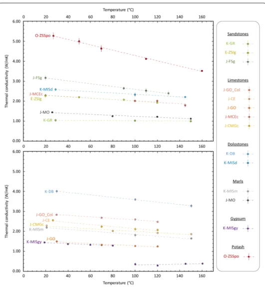
Thermal conductivity is plotted as a function of temperature in Fig. 8, which shows that, for all lithologies, thermal conductivity decreases with increasing temperature.
Fig. 8 Evolution of thermal conductivity of samples in the dry state as a function of temperature. Error bars
indicate standard deviation of thermal conductivity. Colors correspond to lithologies. Names of the samples and trendlines (see Additional file 2 for equations) are indicated. The data are represented in two separate graphs for clarity
Thermal conductivity as a function of temperature is well described by a linear trend (with coefficients of determination, R2, above 0.91; see Additional file 2), apart from gypsum sample K-MISgy above 80 °C (R2 = 0.34; see Additional file 2). Indeed, the K-MISgy gypsum sample shows a decrease similar to that of the other samples below 80 °C but reveals a sharp decrease in thermal conductivity above that limit, from 1.30 W/mK at 80 °C to 0.36 W/mK at 100 °C. Thermal conductivity of the sample slightly increases above 100 °C.
The thermal conductivities of the samples with the lowest thermal conductivities at ambient temperature appear to be influenced less by an increase in temperature. For example, the high-conductivity O-ZSSpo potash sample is more affected (12% conductivity decrease) by a 43 °C temperature increase than the low-thermal-conduc-tivity K-GR sandstone sample is by a 121 °C temperature increase (4% conduclow-thermal-conduc-tivity decrease).
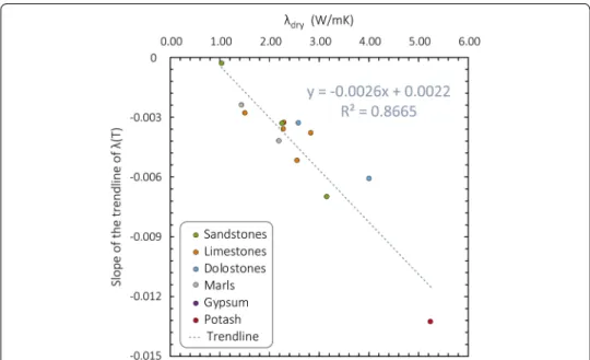
To emphasize the influence of the dry thermal conductivity, the slopes of the linear trends of thermal conductivity as a function of temperature (see Additional file 2 for equations) are plotted as a function of thermal conductivity at ambient temperature in Fig. 9. The K-MISgy gypsum sample is not represented in this graph due to its atyp-ical temperature dependence. This figure shows that the influence of temperature on the thermal conductivity of our sample suite depends on the dry thermal conductivity and that the data can be well described by a linear trend.
Fig. 9 Slope of the trendlines of dry thermal conductivity as a function of temperature (see Fig. 8, equations in Additional file 2) as a function of thermal conductivity of the corresponding sample in the dry state at ambient temperature (λdry). Trendline and corresponding coefficient of determination, R2, are represented. Colors correspond to lithologies. Equation of the trendline is used to estimate thermal conductivity at a given temperature from dry conductivity of the sample
Discussion
The large thermal conductivity and porosity ranges measured in this study suggest that these values are the result of interaction between several parameters. The varia-bility in measured porosities, from near-zero to 44% depending on lithology, indicates that no characteristic value exists for a given lithology. Therefore, a precise measure-ment of the porosity of all rocks is required to properly quantify the influence of this property on thermal conductivity of rocks.
Thermal conductivity
Dry‑state samples at ambient temperature
Thermal conductivity ranges are large for each rock type, highlighting that thermal con-ductivity does not only depend on lithology and there is no characteristic concon-ductivity for a given lithology.
The measurements allowed us to observe a first-order relation between the thermal conductivities of the samples and their porosities for all lithologies: thermal conductiv-ity decreases with increasing porosconductiv-ity as observed in previous studies (Popov et al. 2003; Nagaraju and Roy 2014; Guo et al. 2017; Mielke et al. 2017).
As shown by Fig. 5, the range of thermal conductivity values is small for porous rocks (φ > 25%), regardless of lithology and, thus, composition, which indicates that porosity is a predominant factor controlling thermal conductivity of porous rocks. On the contrary, for less porous rocks (φ < 14%), conductivity values show more variability and depend more on the lithology, which suggests a higher effect of mineralogical composition of the sample.
Saturated‑state samples at ambient temperature
Many studies have shown that measurements on samples in the dry state often under-estimate thermal conductivity of porous rocks due to the low conductivity of air in the pores (Nagaraju and Roy 2014). Furthermore, measurements on saturated samples are often more representative of the in situ conditions since the pore volume is gener-ally filled with water or other liquids that have higher thermal conductivities than air (λwater = 0.6 W/mK) (Nagaraju and Roy 2014; Vosteen and Schellschmidt 2003). The results show an influence of saturation for all the investigated samples. Thermal con-ductivity in the saturated state is generally higher than in the dry state (Fig. 7a). For water-saturated samples, the contrast in thermal conductivity between the rock matrix and the fluid in the pores is smaller than for dry rocks, hence the observed trend for the sedimentary rock samples of this study. However, this trend does not apply to the M-GC shelly sandstone (Grès Coquillier, Muschelkalk), the J-FSg calcareous sandstone
(Forma-tion de Schalkendorf, Jurassic), the J-CE limestone (Calcaire d’Ettendorf, Jurassic) and to
the K-MISgy gypsum (Marnes Irisées supérieures, Keuper). These samples show a low porosity (φ < 10%) and thermal conductivity higher in the dry state than in the saturated state as observed in previous studies by Nagaraju and Roy (2014) and Albert et al. (2017) for sedimentary rocks with porosity smaller than 3%. According to Albert et al. (2017), some rocks react to the fluid used for saturation, resulting in dissolution of some min-eral and/or modification of the structure of the rock matrix of the sample and thus of its thermal conductivity. It is plausible that this phenomenon could have impacted our
samples. The very low porosity of these rocks, and therefore its very low influence of the pore space on conductivity, would have allowed us to observe the decrease in thermal conductivity of the rock matrix due to saturation. For more porous samples, the effect of porosity on conductivity is more significant and could have masked the impact of inter-action between water and the rock matrix.
As shown by Fig. 7b, the effect of water saturation strongly depends on the porosity of the sample and very little on the sample’s mineralogy. This relationship has already been observed in sedimentary rocks by Popov et al. (2003) and Nagaraju and Roy (2014).
However, thermal conductivity measured on saturated samples could not be cor-related with the porosity of the samples. According to Popov et al. (2003), this can be explained by the variability of thermal conductivity of the rock matrix of the studied samples and in particular by the influence of the clay content. In the saturated state, the contrast between thermal conductivity of the matrix and that of the fluid filling the pores is smaller than for dry rocks. It is thus possible that the influence of composition of the rock matrix on thermal conductivity in the saturated state is more important than that of porosity.
Finally, thermal conductivity of the saturated samples is linearly proportional to ther-mal conductivity of the dry samples (Fig. 7c): thermal conductivity in the saturated state increases with increasing conductivity in the dry state, as observed by Guo et al. (2017) for sandstones. This relationship allows us to estimate conductivity of a sample in the water-saturated state at ambient temperature using the dry-state measurement at room temperature (Eq. 8).
Dry‑state samples at high temperature
Many studies have shown that thermal conductivity of dry rocks tends to decrease with increasing temperature (between − 80 and 100 °C by Guo et al. 2017; in the tempera-ture range from 25 to 500 °C by Kant et al. 2017 and between 0 and 300 °C by Vosteen and Schellschmidt 2003). According to Guo et al. (2017), temperature is one of the fac-tors which has the most impact on thermal conductivity of a solid. These studies also showed that the decrease in thermal conductivity with increasing temperature is non-linear. Therefore, performing measurements at relevant in situ temperatures is essential and the experimental conditions should be as close as possible to in situ conditions. This choice is even more important since, in this study, we cannot perform measurements on water-saturated samples at high temperature nor can we study the effect of pressure (closer to in situ conditions) due to equipmental constraints.
The results of high-temperature measurements show an approximate negative linear correlation between thermal conductivity and increasing temperature (Fig. 8 and Addi-tional file 2). It should, however, be emphasized that the temperature ranges chosen for this study (between 18 and 160 °C) are less extensive than the ones considered for the studies previously mentioned. These trends can be used to interpolate/extrapolate ther-mal conductivity at a given temperature for these dry samples and those for which they are used as proxies.
We find that thermal conductivity of dry rocks decreases with increasing tempera-ture, as shown previously by Kant et al (2017), Guo et al. (2017), Vosteen and Schells-chmidt (2003) and Clauser and Huenges (1995). Since, at ambient pressure, the thermal
conductivity of air only increases from 0.025 to 0.036 W/mK as temperature is increased from 20 to 150 °C (Kadoya et al. 1985), we attribute this decrease to changes in the ther-mal conductivity of the rock matrix with increasing temperature. We also cannot rule out decreases in thermal conductivity as a result of increases in porosity due to thermal microcracking (Chaki et al. 2008; Griffiths et al. 2018; Kant et al. 2017) and/or chemical reactions such as the dehydroxylation of clays (Earnest 1991a, b; Mollo et al. 2011), espe-cially at temperatures in excess of 100 °C. The sharp decrease in thermal conductivity of the K-MISgy gypsum above 80 °C can be easily explained by the progressive transfor-mation of gypsum (CaSO4 2H2O) to bassanite (hemihydrate CaSO4 ½H2O) (i.e., par-tial dehydration of gypsum) (Sadeghiamirshahidi and Vitton 2019). The slight increase in thermal conductivity with increasing temperature above this limit can be caused by transformation of the small amount of gypsum that had been left un-transformed in the sample into bassanite.
Yet we observe that some samples are more affected by temperature increase. Ther-mal conductivity of the high-conductivity O-ZSSpo potash decreases more than that of the K-GR sandstone despite a greater temperature increase for the latter. We propose that the higher the initial thermal conductivity measured on a dry sample at room tem-perature, the more it is affected by temperature increase (Figs. 8 and 9) as observed by Vosteen and Schellschmidt (2003). This relationship, which can be satisfactorily charac-terized by a linear trendline (R2 = 0.87), could be used to calculate an estimated thermal conductivity at a given temperature using the dry-state measurements at room tempera-ture (Eq. 5).
Heat flow density estimations
Methods for heat flow density estimations
Based on the various thermal conductivity measurement conditions, three types of heat flow density were calculated for each site: (1) dry rocks at ambient temperature (“dry” heat flow density); (2) dry rocks at in situ temperature (“hot” heat flow density), and (3) saturated rocks at ambient temperature (“wet” heat flow density).
For the dry heat flow density estimates, the thermal conductivities measured on the samples in the laboratory were considered without corrections for in situ temperature or water saturation.
For the hot heat flow density estimates, the thermal conductivities of the samples were either taken directly from the data (if the sample was measured at the in situ tempera-ture) or the thermal conductivity at ambient temperature was corrected for the in situ temperature. To perform this correction, we interpolate/extrapolate the existing data using the empirical relationships defined in this study. For samples measured under dry, hot conditions, the decrease in thermal conductivity with temperature can be described by the following linear equation:
where (T) is the thermal conductivity (in W/mK) at temperature T (in °C), and empiri-cal constants a and b are given by the best-fit linear regression of the data provided in Fig. 8 (equations provided in Additional file 2). The a coefficient of each of the linear trendlines is plotted in Fig. 9 as a function of the dry thermal conductivity at ambient (2) (T ) = aT + b,
temperature, dry , of the associated sample. The best-fit linear regression of this plot pro-vides the following equation:
Thus giving:
The mean measuring temperature of the dry measurements is applied as a correc-tion coefficient for T to average b as measured dry . The thermal conductivity hot at the in situ temperature Tin situ , can therefore be approximated from the dry thermal conductivity at ambient temperature, using the following relation:
For the gypsum-bearing formations, two equations (corresponding to equations of the best-fit linear regressions, Fig. 8 and Additional file 2) were considered to estimate hot thermal conductivity of the gypsum:
Below 80 °C:
Above 80 °C:
For the wet heat flow density estimates, the thermal conductivities of the samples were either taken directly from the data (if the sample was measured in the saturated state) or the thermal conductivity at ambient temperature was corrected for water saturation using the relationship defined by all our wet data (Fig. 7c). The wet thermal conductivity, wet (in W/mK), can be estimated from the dry thermal conductivity at ambient temperature using the following empirical relationship (Fig. 7c):
Samples with a thermal conductivity higher in the dry state than in the water-sat-urated state are not included since thermal conductivity is expected to increase with water saturation.
For the three types of heat flow density, a mean thermal conductivity was calculated for each sedimentary formation observed in the borehole. The composition of the for-mations (proportions of sandstone, marls, dolostone, etc.) was estimated based on the GRT-1 masterlog (Duringer and Orciani (2015), internal report). The mean thermal conductivity of the formation, form , was calculated as the weighted harmonic mean of the thermal conductivities of the samples composing the formation (Beardsmore et al. 2001).
For the formations that were not sampled, the mean thermal conductivity of a forma-tion with similar geological characteristics was used.
(3) a = −0.0026 × dry+0.0022. (4) (T ) = −0.0026 × dry+0.0022 ×T + b. (5) hot= −0.0026 × dry +0.0022 ×(Tin situ−25) + dry. (6) hot= −0.0024 × Tin situ+1.4852. (7) hot=0.001 × Tin situ+0.2337. (8) wet= 0.8496 × dry +0.7524.
The three types of heat flow density were calculated using the equilibrated thermal profiles measured in the wells (Baujard et al. (2017) for Rittershoffen and Genter et al. (2010) for Soultz-sous-Forêts) and the mean thermal conductivities of the formations form . The depths of the limits (top ztop form and bottom zbot form ) of the formations were taken from Duringer et al. (2019) for the Rittershoffen site and from Aichholzer et al. (2016) for the Soultz-sous-Forêts site. The heat flow densities were calculated for each formation between the surface and the top of the Muschelkalk using Fourier’s law:
where qform is the heat flow density of the formation (in W/m2), form is the mean ther-mal conductivity of the sedimentary formation (in W/mK), and Ttop form and Tbot form are the temperatures measured in the well at the top and bottom of the formation, respectively.
For all sites, we define mean heat flow densities for four intervals (1) the whole sedi-mentary cover in the conduction zone (between the surface and the top of the
Muschel-kalk, “global” heat flow density), considered as the “equilibrium” heat flow density and
for the (2) Tertiary, (3) Jurassic and (4) the Keuper intervals to study the evolution of heat flow density with depth.
For each interval, a mean thermal conductivity interval (in W/mK) was calculated as the harmonic mean of the thermal conductivities of the formations within the interval weighted by the thickness of the formations. This mean thermal conductivity was used to calculate qinterval the mean heat flow density (in W/m2) of the considered interval, such as:
where Tbot interval and Ttop interval are the temperatures (in °C) at the top and bottom of the interval, respectively, and zbot interval and ztop interval are the depths (in m) of the top and bottom limits of the considered interval, respectively. A detailed description of the equations and error calculation are provided in Additional file 3.
The first meters of the boreholes were filled with air when the equilibrium-temper-ature profiles were assessed in the geothermal wells. Therefore, the temperequilibrium-temper-ature was considered only where measurements were performed in brine, from depths of 50 and 40.3 meters in GPK-1 and GPK-2, respectively. For GRT-1, the first 149.8 m were not included in the heat flow density calculations.
Estimated heat flow densities
Conductive heat flow density was calculated for each geothermal well (GPK-1 and GPK-2 in Soultz-sous-Forêts and GRT-1 in Rittershoffen) from the equilibrium-tem-perature profiles measured in the wells and from the thermal conductivities measured on (1) dry rocks at ambient temperature (“dry”), (2) dry rock at in situ tempera-ture (“hot”) and (3) saturated rocks at ambient temperatempera-ture (“wet”). The results are
(9) qform= form×Tbot form
−Ttop form zbot form−ztop form
,
(10) qinterval= interval×
Tbot interval−Ttop interval zbot interval−ztop interval ,
presented in Figs. 10, 11 and 12 for GPK-1, GPK-2 and GRT-1, respectively. All the mean values are compiled in Table 1.
The temperature gradient is higher (3–23%) than the global gradient (mean tem-perature gradient of the whole sedimentary column, between the surface and the top
Fig. 10 Stratigraphic log and gamma ray (GR) (after Aichholzer et al. 2016), measured temperature profile T and derived temperature gradient ∆T/∆z (same scale as temperature profile), thermal conductivities λ for dry, hot and wet formations and associated calculated heat flow densities q for the Soultz-sous-Forêts GPK-1 well. Vertical lines indicate mean values for ∆T/∆z (left), λ (middle) and q (right) for a given interval (global (from surface to top of the Muschelkalk), Tertiary, Jurassic and Keuper). Dots indicate average value for a given formation. Stratigraphy is shown in the background for each graph
of the Muschelkalk) in the Tertiary in GRT-1 and in the Jurassic in all the wells. Gra-dients in the other intervals are lower (3–17%) than the global graGra-dients.
For all the wells and all conditions considered, thermal conductivity in the Tertiary interval is always inferior (by 8%) or equal to the global thermal conductivity. The
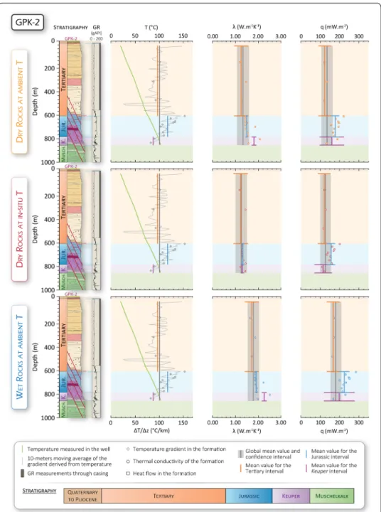
Fig. 11 Stratigraphic log and gamma ray (GR) (after Aichholzer et al. 2016), measured temperature profile T and derived temperature gradient ∆T/∆z (same scale as temperature profile), thermal conductivities λ for dry, hot and wet formations and associated calculated heat flow densities q for the Soultz-sous-Forêts GPK-2 well. Vertical lines indicate mean values for ∆T/∆z (left), λ (middle) and q (right) for a given interval (global (from surface to top of the Muschelkalk), Tertiary, Jurassic and Keuper). Dots indicate average value for a given formation. Stratigraphy is shown in the background for each graph
hot thermal conductivities of the Keuper interval in GRT-1 and GPK-1 are also lower (2–4%) than the global thermal conductivity. Values for the other intervals are higher (4–37%) than the global thermal conductivity.
Fig. 12 Stratigraphic log and gamma ray (GR) (after Duringer et al. 2019), measured temperature profile T and derived temperature gradient ∆T/∆z (same scale as temperature profile), thermal conductivities λ for dry, hot and wet formations and associated calculated heat flow densities q for the Rittershoffen GRT-1 well. Vertical lines indicate mean values for ∆T/∆z (left), λ (middle) and q (right) for a given interval (global (from surface to top of the Muschelkalk), Tertiary, Jurassic and Keuper). Dots indicate average value for a given formation. Stratigraphy is shown in the background for each graph
In the GRT-1 well, the calculated mean global heat flow densities are 122 mW/m2 (± 16%), 109 mW/m2 (± 16%) and 164 mW/m2 (± 12%) for dry, hot and wet rocks, respectively. In GPK-1, the global heat flow densities are 141 mW/m2 (± 18%), 126 mW/m2 (± 18%) and 188 mW/m2 (± 14%) for dry, hot and wet rocks, respectively. In GPK-2, the global heat flow densities are 135 mW/m2 (± 21%), 127 mW/m2 (± 21%) and 181 mW/m2 (± 16%), for dry, hot and wet rocks, respectively.
Heat flow density calculated for the Jurassic in all the wells and for all conditions is higher (9–32%) than the global heat flow density. The same is observed for the hot heat flow density in the Tertiary (3%) and dry heat flow density in the Keuper at Rit-tershoffen (2% higher than global heat flow density) and for the dry and wet heat flow densities in the Keuper for the GPK-1 and GPK-2 wells (3–10% higher). Heat flow densities calculated for all the other intervals are lower (2–26%) than global heat flow density.
In summary, at both sites and under all measurement conditions considered, the mean heat flow densities calculated for the Tertiary always fall within the range of variability of the mean global heat flow densities. The same applies for the Keuper in GRT-1 in the dry and wet conditions and for the mean hot and wet heat flow densi-ties in the Jurassic. The mean value calculated for the Jurassic at Rittershoffen for dry rocks is too high to be in the range of variability of the global dry heat flow density. Hot heat flow density in the Keuper is too low to be in the range of variability of the hot mean value.
At Soultz-sous-Forêts, the mean heat flow densities calculated in the Jurassic are sys-tematically out of the interval of the global heat flow densities in GPK-1 and GPK-2. The hot heat flow density calculated in the Keuper in GPK-1 is also too low to be within the
Table 1 Mean calculated thermal conductivities λ and heat flow densities q for the various intervals in the GRT-1, GPK-1 and GPK-2 geothermal wells
Mean measured temperatures and temperature gradients are given for the various intervals [global (from surface to top of the Muschelkalk), Tertiary, Jurassic and Keuper]. Data for dry rocks at ambient temperature (dry), dry rocks at in situ temperature (hot) and saturated rocks at ambient temperature (wet)
Well Interval Mean T
(°C) ∆T/∆z (°C/100 m) Dry Hot Wet
Mean λ (W/
mK) Mean q (mW/m2) Mean λ (W/mK) Mean q (mW/m2) Mean λ (W/mK) Mean q (mW/ m2) GRT-1 Global 92.54 9.07 1.35 ± 0.20 122 ± 19 1.20 ± 0.18 109 ± 18 1.81 ± 0.19 164 ± 20 Tertiary 71.59 9.32 1.25 ± 0.24 117 ± 24 1.20 ± 0.24 112 ± 24 1.71 ± 0.23 159 ± 24 Jurassic 132.30 9.69 1.49 ± 0.04 144 ± 18 1.22 ± 0.05 118 ± 16 1.90 ± 0.05 184 ± 22 Keuper 153.25 7.03 1.77 ± 0.07 125 ± 31 1.15 ± 0.07 81 ± 22 2.27 ± 0.08 160 ± 39 GPK-1 Global 64.49 10.13 1.40 ± 0.24 141 ± 26 1.25 ± 0.21 126 ± 23 1.85 ± 0.23 188 ± 26 Tertiary 46.02 10.08 1.25 ± 0.30 126 ± 32 1.23 ± 0.30 124 ± 32 1.71 ± 0.29 172 ± 32 Jurassic 83.07 12.46 1.50 ± 0.05 187 ± 22 1.32 ± 0.06 165 ± 21 1.91 ± 0.05 238 ± 25 Keuper 101.54 8.37 1.85 ± 0.06 155 ± 24 1.22 ± 0.06 102 ± 17 2.32 ± 0.09 194 ± 31 GPK-2 Global 62.34 10.14 1.33 ± 0.26 135 ± 29 1.26 ± 0.25 127 ± 27 1.78 ± 0.25 181 ± 28 Tertiary 49.00 9.78 1.25 ± 0.31 123 ± 33 1.23 ± 0.32 120 ± 33 1.71 ± 0.31 167 ± 33 Jurassic 87.60 11.82 1.50 ± 0.05 177 ± 21 1.32 ± 0.06 157 ± 20 1.90 ± 0.05 225 ± 25 Keuper 100.95 8.81 1.82 ± 0.10 160 ± 63 1.31 ± 0.07 115 ± 45 2.26 ± 0.12 199 ± 77
range of variability of the hot global value. The other values are within the interval of confidence of the global heat flows.
Influence of the thermal‑conductivity‑measurement conditions
The dry heat flow densities calculated using the new thermal conductivities values measured in this study on samples from the URG are similar to the previously pub-lished heat flow densities for the Soultz-sous-Forêts site and close to Rittershoffen. The heat flow at Soultz-sous-Forêts was estimated in previous studies to be between 140 and 150 mW/m2 (Flores Marquez 1992; Le Carlier et al. 1994; Schellschmidt and Clauser 1996; Pribnow and Clauser 2000; Baillieux et al. 2013) and we estimate here heat flow densities of 141 ± 18 mW/m2 for GPK-1 (Fig. 10 and Table 1) and 135 ± 21 mW/m2 for GPK-2 (Fig. 11 and Table 1). The heat flow density estimated near the Rittershoffen site, 121 mW/m2, compares well with our estimated value of 122 ± 16 mW/m2 for GRT-1 (Fig. 12 and Table 1).
Our results also show that heat flow density depends strongly on thermal conduc-tivity measurement conditions. Heat flow densities calculated using the thermal con-ductivities of water-saturated rocks at ambient temperature can be up to 43% higher than heat flow densities calculated for dry rocks (dry rocks at ambient temperature) (Table 1), and heat flow densities calculated using values measured on hot rocks (dry rocks at in situ temperature) can be up to 11% lower than “dry” heat flow densities (Table 1). Since the “dry” rock scenario is likely the least realistic, these results proba-bly do not represent the true heat flow density values. Further, dry heat flow densities were already discussed for Soultz-sous-Forêts in previous studies, henceforth we only discuss the hot and wet heat flow density models determined by our study.
It is still unclear whether the in situ rocks are saturated or not; verifying the rock satu-ration at depth in the geothermal wells is particularly complicated. We therefore cannot conclude on the validity of the wet heat flow densities but, as stated, the effect of satura-tion of the rocks on the calculated heat flow density should not be ignored. The effect of temperature increase down the borehole, however, is undeniable. Temperature increases with depth, and as shown before, thermal conductivity of rocks decreases with increas-ing temperature. Consequently, we cannot assert that considerincreas-ing hot rocks is more rep-resentative than considering wet rocks since it is very plausible that some formations are both hot and saturated while some others are still effectively dry at the in situ tempera-ture conditions. Although the effect of pressure could not be accounted for, we conclude that the hot and wet heat flow densities calculated for the URG using the thermal con-ductivity data presented herein are more representative of the in situ conditions than the dry heat flow densities previously calculated.
Evolution of the heat flow density with depth
In a sedimentary basin in which heat transfer is mostly driven by conduction, heat flow density should remain approximately constant with depth (Andrews-Speed et al. 1984; Schütz et al. 2014). Therefore, examining the vertical heat flow density variations with depth at Soultz-sous-Forêts and Rittershoffen should enable us to investigate conductive equilibrium down the geothermal wells. Heat flow density is considered constant if the intervals of confidence of the heat flow density values in the various intervals (Tertiary,
Jurassic and Keuper) overlap those of the global heat flow densities (over the whole conduction zone). Variations for the dry heat flow densities will not be discussed here, because, as stated earlier, dry conditions were already investigated by previous studies (Baillieux et al. 2013; Flores Marquez 1992; Pribnow and Clauser 2000; Le Carlier et al. 1994; Schellschmidt and Clauser 1996; Pribnow and Schellschmidt 2000).
In the GRT-1 well, the error bars of the hot or wet heat flow densities over the Ter-tiary, Jurassic and Keuper intervals all overlap the interval of confidence of the calcu-lated global hot or wet heat flow densities (Table 1 and Fig. 12). Thus, we consider the conductive heat flow density in GRT-1 to be constant for the whole sedimentary cover between the surface and the top of the Muschelkalk; equilibrium thermal conduction of heat controls the evolution of temperature with depth over this interval. At Soultz-sous-Forêts, with the exception of the wet value for the Jurassic in GPK-2, the error bars of the hot or wet heat flow densities over the Tertiary, the Jurassic and the Keuper intervals all overlap the confidence interval of the global hot or wet heat flow densities (Table 1 and Figs. 10, 11). However, the calculated absolute values of the Jurassic interval in the hot and wet conditions are systematically higher (2–11%) than the upper boundary of the global heat flow densities. This anomaly is only observed for the Soultz-sous-Forêts site, in both GPK-1 and GPK-2. Even though errors on the calculated heat flow densities values are large (about 12% in the Jurassic), the difference between the heat flow densi-ties in the Jurassic and the global heat flow densidensi-ties are probably significant.
It is necessary here to understand if this recurrent heat flow density anomaly in the Jurassic intersected by the Soultz-sous-Forêts wells is real or the result of a systematic error. The method used in this study is the victim of many sources of errors. First, it is possible that when temperature logs were performed in the wells, the systems were not at thermal equilibrium with the surrounding geological formations (Bullard 1947). The temperature log from GPK-1 used to calculate the heat flow density was measured in June 1997, more than 7 months after hydraulic circulation tests in the wells. In GPK-2, temperature was assessed in July 1999, 3 months after the end of the deepening drilling operations in the granitic basement, the sedimentary cover was already fully cased at that time. These periods without perturbations in the wells should have allowed tem-perature in the boreholes to equilibrate with the host rocks. Temtem-perature logs in Soultz-sous-Forêts are thus considered to be as close as possible to equilibrium (Genter et al. 2010).
Second, the local anomaly in the Jurassic could be induced by the rock sampling method. The temperature logs in Soultz-sous-Forêts indeed reveal a higher gradient in the Jurassic than in the Tertiary or in the Keuper intervals (Table 1 and Figs. 10, 11) (Pribnow and Schellschmidt 2000). Maintaining a constant heat flow density over the three intervals would require lower thermal conductivity values than those measured in the laboratory on the Jurassic samples. There are several possible sources of error due to sampling method. (1) Some formations cannot be cored in a way that allows ther-mal conductivity measurements, especially in the Jurassic, due to friability of the mate-rial. We therefore chose to sample analogue rocks from accessible outcrops, which can feature (thermal) properties different from that of the in situ rocks (Bauer et al. 2017). (2) Not all samples could be measured saturated or at in situ temperature; instead, the hot and wet thermal conductivities are interpolated/extrapolated using the here-defined
empirical relationship (Figs. 7c, 9 respectively). These empirical relationships may intro-duce significant errors when estimating hot or wet thermal conductivities and more measurements are required to further refine these equations. Further, the effect of pres-sure could not be studied on our samples. Based on previous studies (Walsh and Decker 1966; Abdulagatova et al. 2009; Schön and Dasgupta 2015), we would expect pressure to reduce porosity and close microcracks and thus increase thermal conductivity, but the extent of that effect coupled to that of temperature and saturation remain to be quanti-fied for the rocks of the URG. (3) For formations that could not be sampled, the sam-pled formations were used as proxies. For example, the J-MO sample was sourced from a quarry and was used as an analogue for almost all the marls from the Jurassic; this choice to use an analogue rock may induce errors in thermal conductivity estimates. Yet, we note that the thermal conductivity of the marls at the base of the Jurassic (J-CMGm,
Calcaires et Marnes à Gryphées) is not very different from that of the J-MO marls
(Addi-tional file 1). We thus consider that the use of these analogues materials as a proxy for all the marls of the Jurassic can be justified.
Third, the composition of the formations (proportions of lithology) was estimated from the GRT-1 masterlog (Duringer and Orciani (2015), internal report). The masterlog itself can bear errors if part of the material in the rock cuttings was lost during clean-ing (for example, a greater proportion of marls in the in situ formation than observed in the washed cuttings). Also, the masterlog from the Rittershoffen well might not be completely applicable to the Soultz-sous-Forêts geology due to lateral variation of facies in the formations (Fuchs 2018). However, it is very unlikely that facies of the Triassic and Jurassic formations drastically change over 6 km of horizontal distance (between Ritter-shoffen and Soultz-sous-Forêts) as shown by Aichholzer et al. (2016).
While direct downhole measurements of thermal conductivity under in situ condi-tions are the most applicable and would allow us to verify the reliability of the values measured on outcrop samples, such measurements are rare and more expensive than laboratory measurements (Garibaldi 2010; Harcouët 2005).
Further, paleoclimatic and/or topographic corrections are usually required for heat flow density estimates (Beck 1977; Blackwell et al. 1980; Guillou-Frottier et al. 1998; Jae-ger and Sass 1963; Lucazeau and Vasseur 1989; Luijendijk et al. 2011; Majorowicz and Wybraniec 2011; Mareschal et al. 2000; Vasseur 1980) and uncorrected data can yield errors in estimated heat flow densities.
Nevertheless, the gradient in the Jurassic interval of the Soultz-sous-Forêts wells is noticeably higher than in the Rittershoffen well, which leads us to believe that this anomaly cannot only be induced by variations in rock thermal conductivities between the two sites. If the methods are not a source of error, then the heat flow density anomaly observed in the Jurassic interval at Soultz-sous-Forêts could be explained by at least four processes: radiogenic heat production, non-equilibrium conduction of heat, heat flow density refraction or transfer of heat by nonconductive processes.
Radiogenic heat production can contribute significantly to surface heat flow density in sedimentary basins (Frone et al. 2015; Guillou-Frottier et al. 2010; Schütz et al. 2012; Waples 2002). In sediments, radiogenic heat production can be high in some shales especially in those rich in organic matter, like in the black shales of the Toarcian (Juras-sic) encountered in the URG (Böcker et al. 2017; Böcker and Littke 2016; Waples 2002).