On the changing seasonal cycles and trends of ozone at Mace Head, Ireland

(1)

HAL Id: hal-00301698

https://hal.archives-ouvertes.fr/hal-00301698

Submitted on 15 Aug 2005

HAL is a multi-disciplinary open access

archive for the deposit and dissemination of sci-entific research documents, whether they are pub-lished or not. The documents may come from teaching and research institutions in France or abroad, or from public or private research centers.

L’archive ouverte pluridisciplinaire HAL, est destinée au dépôt et à la diffusion de documents scientifiques de niveau recherche, publiés ou non, émanant des établissements d’enseignement et de recherche français ou étrangers, des laboratoires publics ou privés.

On the changing seasonal cycles and trends of ozone at

Mace Head, Ireland

D. C. Carslaw

To cite this version:

D. C. Carslaw. On the changing seasonal cycles and trends of ozone at Mace Head, Ireland. Atmo-spheric Chemistry and Physics Discussions, European Geosciences Union, 2005, 5 (4), pp.5987-6011. �hal-00301698�

(2)

ACPD

5, 5987–6011, 2005

Changing seasonal ozone cycles at Mace

Head D. C. Carslaw Title Page Abstract Introduction Conclusions References Tables Figures J I J I Back Close

Full Screen / Esc

Print Version Interactive Discussion

EGU Atmos. Chem. Phys. Discuss., 5, 5987–6011, 2005

www.atmos-chem-phys.org/acpd/5/5987/ SRef-ID: 1680-7375/acpd/2005-5-5987 European Geosciences Union

Atmospheric Chemistry and Physics Discussions

On the changing seasonal cycles and

trends of ozone at Mace Head, Ireland

D. C. Carslaw

Institute for Transport Studies, University of Leeds, Leeds LS2 9JT, UK

Received: 3 June 2005 – Accepted: 26 July 2005 – Published: 15 August 2005 Correspondence to: D. C. Carslaw (d.c.carslaw@its.leeds.ac.uk)

(3)

ACPD

5, 5987–6011, 2005

Full Screen / Esc

EGU

Abstract

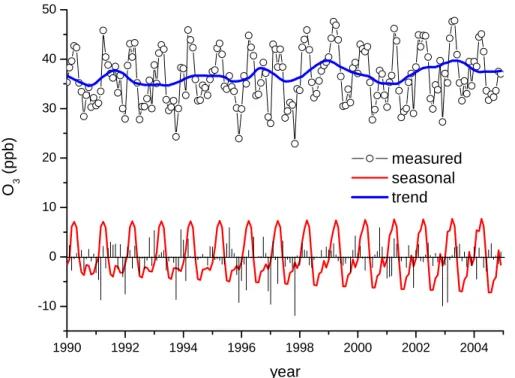
A seasonal-trend decomposition technique based on a locally-weighted regression smoothing (Loess) approach has been used to decompose monthly ozone concen-trations at Mace Head (Ireland) into trend, seasonal and irregular components. The trend component shows a steady increase from 1990–2004, which is confirmed by

5

statistical testing that shows that ozone concentrations at Mace Head have increased at the p=0.06 level by 0.18±0.04 ppb yr−1. By considering different air mass origins using a trajectory analysis, it has been possible to separate air masses into “polluted” and “unpolluted” origins. The seasonal-trend decomposition technique confirms the different seasonal cycles of these air mass origins with unpolluted air mass maxima

10

in April and polluted air mass maxima in July/August. A detailed consideration of the seasonal component reveals different behaviour depending on the air mass origin. For baseline unpolluted air arriving at Mace Head there has been a gradual increase in the seasonal amplitude, driven by a declining summertime component. The amplitude of the seasonal component of baseline air is controlled by a maximum in April and a

mini-15

mum in July. For polluted air mass trajectories, there was a substantial reduction in the amplitude of the seasonal component from 1990–1997. However, post-1997 results indicate that the seasonal amplitude in polluted air masses arriving at Mace Head is increasing. Furthermore, there has been a shift in the months controlling the size of the seasonal amplitude in polluted air from a maximum in May and minimum in January in

20

1990 to a maximum in April and a minimum in July by 2001. These results indicate that the characteristics of baseline air are becoming more important in polluted air masses arriving at this location.

1. Introduction

There is considerable interest in tropospheric ozone for many reasons. On a local to

25

(4)

ACPD

5, 5987–6011, 2005

Full Screen / Esc

EGU parts of the world. Additionally, ozone is damaging to agricultural crops, forests and

materials (Fowler et al., 1999). Ozone is also the third most important greenhouse gas and is the principal source of the hydroxyl radical (Houghton et al., 2001). The seasonal cycle of ozone in the troposphere is controlled by a wide range of chemical and dynamical processes (Scheel et al., 1997; Monks, 2000). One of the most

dis-5

tinctive characteristics of the ozone seasonal cycle in the Northern Hemisphere is the springtime maximum, which has been extensively investigated (Derwent et al., 1998b; Monks, 2000; Wang et al., 2003). Recently, global models and measurement cam-paigns have highlighted the extent to which ozone is a trans-continental problem. Li et al. (2002) using the GEOS-CHEM model found that North American anthropogenic

10

emissions contribute 5 ppb ozone on average at Mace Head on the west coast of Ire-land. Derwent et al. (2004) using the STOCHEM model suggest that about 12 ppb ozone at Mace Head is North American in origin and about 7 ppb is Asian, compared with a total modelled concentration of 41 ppb for annual mean daily maximum ozone concentrations. In Europe there has been a reduction in ozone precursors leading to

15

a reduction in peak summertime ozone concentrations (Derwent et al., 2003). Ozone concentrations have also been shown to increase as a result of biomass burning events (Honrath et al., 2004; Simmonds et al., 2005). At remote locations such as Mace Head, it has been observed that ozone concentrations are increasing in tropospheric baseline air masses (Simmonds et al., 2004).

20

These influences would be expected to affect the seasonal cycle of ozone concen-tration in different ways. For example, the reduction in precursor emissions in Europe would be expected to reduce peak summertime ozone concentrations. Conversely, reduced concentrations of NO_X in Europe would tend to result in less ozone titration through the O₃+NO reaction, particularly during the winter, thus leading to increased

25

wintertime ozone concentrations. On the other hand, transport of ozone from North America tends to be most important during the spring and autumn, coinciding with pe-riods of efficient ozone production, long ozone lifetime and fast transport (Wang et al., 1998; Li et al., 2002). These factors all potentially affect the ozone seasonal cycle in

(5)

ACPD

5, 5987–6011, 2005

Full Screen / Esc

EGU terms of the timing of peaks or troughs, the amplitude and the seasonal trend. For

these reasons it can be useful to focus specifically on the seasonal aspects of ozone concentration as a method of recording and understanding the factors controlling ozone concentrations.

There are many approaches available to extract the seasonal and trend components

5

from time series. Traditional approaches decompose a time series into a long term component and an additive seasonal component and assume that seasons differ only in magnitude. The additive assumption is often inappropriate for air pollution data be-cause seasonal effects can have a different forcing over time. Given the importance of the seasonal cycle to ozone concentrations, discerning systematic changes to the

sea-10

sonal pattern is essential to developing an understanding of the processes controlling ozone concentrations and changes in concentration over time. For this reason a more flexible approach is required.

Much of the motivation for time series decomposition derives from the analysis of economic data where information, such as unemployment rates, is expressed as

sea-15

sonally adjusted (Franses, 1996). An extensively used empirical method, known as X-11, has been applied for several decades to produce official statistics by various governments and institutions. The method was introduced in 1965 by the US Cen-sus Bureau and has undergone many developments (Shiskin et al., 1967). Latterly, the method has been developed to include Autoregressive Integrated Moving Average

20

(ARIMA) modelling to improve “end-effect” problems and extensive statistical diagnos-tic tools (Dagum, 1980; Findlay et al., 1998). The X-11 method decomposes a time series into a trend, seasonal and irregular component through the use of trend and seasonal moving average filters. Recently, the X-11 approach has been used to high-light the seasonal variability sea surface temperatures (Pezzulli et al., 2005).

Model-25

based approaches have also been used to examine changes in ozone seasonality at Jungfraujoch in Switzerland, where a state-space method was applied (Schuepbach et al., 2001). The state-space approach showed that there had been a statistically significant negative trend in May ozone from 1988–1997, which was not statistically

(6)

ACPD

5, 5987–6011, 2005

Full Screen / Esc

EGU significant when ordinary linear regression was used.

In the current work, a seasonal-trend decomposition technique is used to extract the seasonal and trend components of ozone for different air mass origins at Mace Head, Ireland. A locally weighted regression (Loess) method of seasonal trend decomposition (STL) is used that provides a nonparametric means of describing nonlinear trends and

5

seasonal cycles. STL was used in preference to X-11 because of the ease with which STL can be modified for specific applications. By employing methods that aim to extract different components of the ozone time series, attention can be focussed on different aspects of the ozone seasonal cycle and trends.

2. Data and methods

10

2.1. Measurement data and site description

Mace Head is situated at a coastal location on the west coast of Ireland at 53◦N, 10◦W, with a sampling height 25 m above sea level (Cvitas and Kley, 1994). The station is part of the Advanced Global Atmospheric Gases Experiment (AGAGE), as well as being a EUROTRAC/TOR (Tropospheric Ozone Research) station (Simmonds et al., 1996).

15

The location of Mace Head is ideally suited for the analysis of different air mass origins. For the majority of the time Mace Head is influenced by air masses that have travelled across the North Atlantic with a fetch of several thousand kilometres. The analysis of trace gas data at Mace Head can therefore provide an insight into global background concentrations (e.g. Derwent et al., 1998a, b; Simmonds et al., 2004). Mace Head is

20

also affected less frequently by more polluted air masses that derive from European sources. An important aspect of this location therefore is the potential to investigate tropospheric background air and air that has been strongly influenced by anthropogenic sources.

Ozone measurements at Mace Head were made with a commercial Monitor Labs

25

(7)

ACPD

5, 5987–6011, 2005

Full Screen / Esc

EGU calibrated every three months against a primary UV photometer. Ozone measurements

are recorded as hourly means, from which monthly means were calculated. The data set used covered a period from January 1990 to December 2004.

2.2. Seasonal-trend decomposition using Loess

A time series can be considered to comprise three components: a trend component

5

T (m), a seasonal component S(m) and a remainder R(m), sometimes referred to as

the irregular component:

Y (m)= T (m) + S(m) + R(m) (1)

Where Y (m) is the time series of interest.

The locally weighted regression smoothing technique (Loess) developed by

Cleve-10

land (1979) has been widely used in data analysis. The Loess technique has also been developed as a tool for seasonal-trend decomposition (STL – seasonal-trend decom-position using Loess) (Cleveland et al., 1990). The STL method consists of a series of applications of a Loess smoother with different moving window widths chosen to extract different frequencies within a time series. The nonparametric nature of STL makes it

15

suitable for dealing with non linear trends. Furthermore, the STL approach provides an effective graphical analysis of the different time series components, which is useful for diagnostic checking. The technique is also able to deal with missing data.

The STL method involves an iterative algorithm to progressively refine and improve estimates of the trend and seasonal components. STL consists of two recursive

pro-20

cedures, one nested within the other, called the inner loop and the outer loop. Each pass of the inner loop applies seasonal smoothing that updates the seasonal compo-nent, followed by trend smoothing that updates the trend component. An iteration of the outer loop consists of one or two iterations of the inner loop followed by an identifi-cation of extreme values. Further iterations of the inner loop down-weight the extreme

25

values that were identified in the previous iteration of the outer loop. Typically, less than 10 iterations of the outer loop are carried out to ensure convergence. Because each

(8)

ACPD

5, 5987–6011, 2005

Full Screen / Esc

EGU month is a sub-series in the Loess fitted model, changes in the seasonal effects are

captured. This attribute makes STL an effective tool for investigating seasonal ozone trends where there are likely to be different influences affecting the seasonal ozone cycle over time. The statistical robustness of the STL method is also a useful attribute when applied to concentrations of atmospheric species that are often influenced by

5

events such as pollution episodes leading to outliers, which could adversely affect the clean extraction of an underlying trend or seasonal component.

There are several important parameter choices that must be made in STL. Many depend on the individual data sets being processed (e.g. whether daily or monthly data are used). Probably the most important choice is the value for the seasonal

10

smoothing parameter, n(s). As n(s) increases, each cycle sub-series (e.g. the series of all January values in a monthly data set) become smoother. The choice of parameters should also ensure that the seasonal and trend components do not compete for the same variation in the data. Furthermore, parameters are chosen such that long-term oscillations are represented in the trend component and not the remainder. Cleveland

15

et al. (1990) recommend a series of graphical diagnostic methods to determine the choice of parameters in STL, which have been followed in this study.

3. Results and Discussion

3.1. Analysis of Mace Head ozone data

Figure 1 shows the results of applying the technique to monthly ozone data from Mace

20

Head. Figure 1 shows that the trend component has been slowly increasing from 1990–2004, while also highlighting other long-term features. The peak in the trend component in 1998/99 is likely to relate to biomass burning for example (Simmonds et al., 2004). The seasonal component shows a peak around April and a minimum around July each year. The amplitude of the seasonal component is also shown to increase

25

(9)

ACPD

5, 5987–6011, 2005

Full Screen / Esc

EGU of data for each month that is not described by either the trend or seasonal

compo-nents. The remainder component contains, for example, periods that are affected by short-term air pollution episodes, such as those shown by the negative values in Jan-uary and November 1997. An analysis of the components in Fig. 1 shows that most of the variance is in the seasonal component and the least in the trend. As the time

5

scale reduces, for example, to a weekly time series, the variance in the remainder term increases to be approximately equal to that of the seasonal component. For monthly data therefore, the seasonal component is the most important characteristic controlling the variation in ozone concentrations.

The non-parametric seasonal Mann-Kendall analysis was applied to the measured

10

monthly mean ozone concentrations from 1990–2004 to determine whether there was a significant change in the trend (Hirsch et al., 1982). These results showed that there has been a statistically significant upward trend in ozone concentrations over this pe-riod at the p=0.06 level. An analysis of the extracted trend component suggests an in-crease of 0.18±0.04 ppb yr−1. The most significant increases (p<0.10) were observed

15

for March–May and November. Non-significant decreases in ozone were predicted for July, August and September. Overall, increases in ozone for different months were more statistically significant than any decreases.

Ozone data at Mace Head have previously been filtered depending on air mass ori-gin (Derwent et al., 1998b; Prinn et al., 2000; Simmonds et al., 2004). Simmonds et

20

al. (2004) presented three techniques: pollution filtering based on the concentrations of different trace gases, trajectory analysis and the use of a Lagrangian model. The method adopted presently is filtering based on an analysis of EMEP (Co-operative pro-gramme for monitoring and evaluation of the long range transmission of air pollutants in Europe) back trajectories. With this method, back trajectories are followed for 96 h at

25

a pressure height of 925 hPa. The area around the arrival point is divided into 8 equal sectors of 45◦. North (N) is defined as being centred on 0◦, north-east (NE) centred on 45◦etc. Days are allocated to a particular sector if at least 50% of the trajectory posi-tions are found within that sector. If trajectories cannot be assigned in this way they are

(10)

ACPD

5, 5987–6011, 2005

Full Screen / Esc

EGU classified as unattributable. Derwent et al. (1998a) defined “unpolluted” or baseline air

as deriving from N, NW, W and SW, which is also the assumption made here. Polluted air masses from Europe were assumed to derive from wind sectors NE, E, SE and S. Data were available from 1990–2001. Over the period 1990–2001, 54% of conditions were classified as baseline, 14% polluted and 32% were unattributable. A

disadvan-5

tage of the trajectory allocation approach is the large proportion of unattributable tra-jectories. However, these are considered further in Sect.3.3, where the characteristics of these air masses are compared with baseline and polluted air masses.

Figure 2a–c shows the seasonal component extracted for three different air mass types using the STL technique. For baseline air arriving at Mace Head (Fig. 2a) there

10

is some evidence that the amplitude of the seasonal cycle is increasing. Furthermore, the ozone maximum in April each year broadens into February. The summertime min-imum observed in baseline air at Mace Head is believed to be partly explained by long-range transport from more southerly latitudes and the photochemical destruction of ozone in a low-NO_X environment (Scheel et al., 1997). For air masses from a

pol-15

luted origin (Fig. 2b), the seasonal cycle is less smooth. There also appears to be a reduction in the amplitude of the seasonal component, caused primarily by an increas-ing wintertime ozone component. The peak in May remains approximately constant but there is some suggestion in Fig. 2b that this peak increases towards the end of the time series. Air masses from the polluted sectors also incorporate an important contribution

20

from baseline air. Therefore, the difference (polluted minus baseline) seasonal compo-nent is considered. Fig. 2c shows this difference and highlights a clear reduction in the seasonal component amplitude from 1990–2001. The variations in these amplitudes and seasonal components are considered more in Sect. 3.3.

The seasonal time series presented in Fig. 2 have been analysed to derive the mean

25

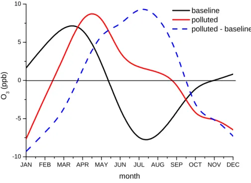
monthly variation in the seasonal components of the different air mass origins. Figure 3 shows the monthly variation averaged over 1990–2001. For baseline air trajectories, there is a clear peak in the seasonal component in March/April and a minimum in July/August. The polluted air mass trajectories peak later in April/May and have their

(11)

ACPD

5, 5987–6011, 2005

Full Screen / Esc

EGU minimum in December/January. The polluted minus baseline seasonal component has

a very different variation, with a clear peak in July/August and a minimum in Decem-ber/January. The latter plot appears to highlight summertime ozone production that would be expected in polluted air masses from Europe. These results also provide some evidence that the allocation into baseline and polluted air mass origins using the

5

EMEP daily sector methodology adequately distinguishes between air masses with different characteristics.

The slope of the extracted trend component for each of the time series by air mass origin was calculated using a linear regression. For baseline air a 0.25±0.06 ppb yr−1 (at a 95% confidence interval) increase in ozone was calculated from 1990–2001.

10

For polluted air masses no change in the slope was calculated from 1990–2001 (0.01±0.10 ppb yr−1). For air mass trajectories from a polluted direction it appears that increases in the baseline ozone over 12 years have been offset by decreases in ozone from polluted i.e. European air masses. The increase in baseline ozone of 0.25±0.06 ppb yr−1 using the STL approach is in good agreement with that calculated

15

by Simmonds et al. (2004) of 0.30±0.25 ppb yr−1using the EMEP daily allocation tech-nique, for data from April 1987 to March 2003. Although not shown, the slope of the trend in the unallocated air mass trajectories was 0.20±0.07 ppb yr−1, which is closer to the slope for baseline air than polluted air. Given that baseline air trajectories account for 54% of the air masses arriving at Mace Head and polluted 14%, it seems

reason-20

able to expect the unallocated trajectories to be dominated by baseline air. These slopes for the different air mass components (baseline, polluted and unallocated) are consistent with an overall trend of 0.18±0.04 ppb yr−1. The preferred pollution filtering technique used by Simmonds et al. (2004) did, however, yield greater rates of growth for both baseline and polluted air masses (0.49±0.19 ppb yr−1and 0.40±0.32 ppb yr−1,

25

respectively). In the context of the current work, these growth rates appear to be too high.

(12)

ACPD

5, 5987–6011, 2005

Full Screen / Esc

EGU 3.2. Changes to the seasonal component

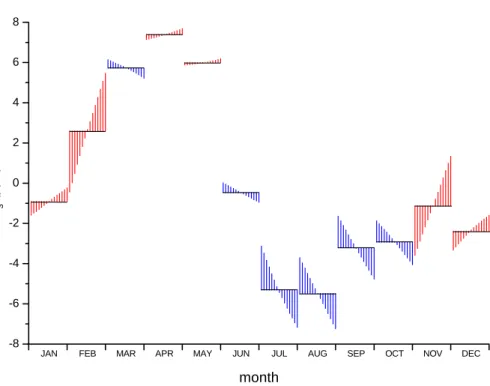
Even though the seasonal plots shown in Fig. 2 portray useful information, it is di ffi-cult to assess the behaviour of each cycle sub-series. A better interpretation of the seasonal component can be gained by plotting the cycle sub-series to highlight the characteristics of the seasonal component (Cleveland et al., 1990). Figure 4 shows the

5

cycle sub-series of the monthly Mace Head data. First, the January values are plotted for successive years, then the February values, and so on. The individual values of a sub-series are shown as a series of vertical lines about the mean of the sub-series. The sub-series plot allows for an assessment of the magnitude of the seasonal component (as shown by the horizontal line for each month) and the behaviour of each monthly

10

sub-series. Figure 4 shows for example, that April represents the month of the highest seasonal component and August the smallest. It also shows that the wintertime sea-sonal component is tending to increase, whereas for most summertime months there is a decrease with time. The increase in the seasonal component is most apparent for February and November. Conversely, the greatest decreases are most apparent in

15

July and August. In addition, because all values shown in Fig. 4 are on the same scale, it is possible to determine whether the changes to any monthly sub-series are small or large compared with the month to month variation in the seasonal component. On this basis the changes shown for February and November appear to be large compared with the variation from month to month.

20

3.3. Estimation of the uncertainties to changes in the seasonal component

Section 3.2 highlighted how changes in the seasonal cycle of ozone at Mace Head have changed over the past 15 years, characterised by an increasing wintertime and decreasing summertime component. The changes shown in Fig. 4 for the seasonal ozone cycle are, however, subject to uncertainty. Monte Carlo simulations were carried

25

out to estimate the errors in the change in the seasonal component as shown by Fig. 4 and changes in the amplitude in the seasonal cycle shown in Fig. 1. The remainder

(13)

ACPD

5, 5987–6011, 2005

Full Screen / Esc

EGU component, R(m), was used to describe the noise in the time series. An analysis of

R(m) in Fig. 1 by considering the correlegram showed that the series appeared to be

random, with no obvious lag-effects. The R(m) was also close to a normal distribution, with a mean close to zero. The R(m) was, however, found to have a larger variance dur-ing the winter months for each time series, probably as a result of wintertime pollution

5

episodes. Therefore, σ2 was used to describe the seasonal variance of the residual term (shown in Table 1), and σ2(m) the time series of the residual term over the entire length of the data set. Table 1 shows that the error term σ tends to be higher for the autumn and winter periods compared with the spring and summer periods for most air mass types. Table 1 also shows that for baseline air there is little variation in the error

10

term throughout the year, probably as a result of the reduced number of regional pol-lution episodes affecting these air mass trajectories. In general, the polluted air mass trajectories show increased value in the noise term. A large number of time series,

Y (m)∗, were constructed:

Y (m)∗= T (m) + S(m) + W (m)∗ (2)

15

where T (m) and S(m) are the trend and seasonal components for the same series, derived from the decomposition of the original series, and W (m)∗ is described as a Gaussian white noise series with a mean of zero and a variance σ2(m), derived from a Gaussian random number generator.

Simulations were undertaken to estimate the error terms in the seasonal amplitude

20

and seasonal change as follows. First, a series of 500 synthetic ozone datasets were generated using Eq. (2) for 180 months of Mace Head ozone data shown in Fig. 1 (the length of the dataset). This process yielded 500 new time series, which were then de-composed using the STL method. This approach was also applied to the shorter time series (144 months) for the Mace Head baseline, polluted and unallocated air mass

tra-25

jectories. For each of the new time series, the amplitudes of the seasonal component were calculated as the maximum S(m) subtracted from the minimum S(m) for each calendar year. The standard error of the amplitude for each year was calculated from the 500 amplitude predictions. The change in the seasonal component was expressed

(14)

ACPD

5, 5987–6011, 2005

Full Screen / Esc

EGU as the last monthly value in each time series minus the first e.g. January 2004 minus

January 1990 for the full Mace Head time series. The standard error associated with the seasonal change was also calculated.

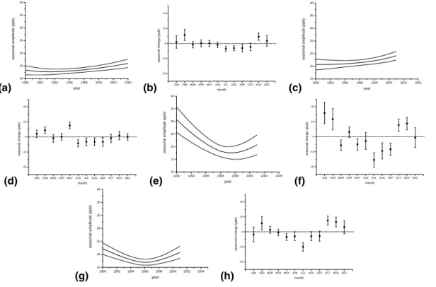
Figure 5 shows the results for the changes in the seasonal amplitude and the sea-sonal change trend with associated errors for the different air mass types. Figure 5a

5

shows that for the full Mace Head ozone dataset the seasonal amplitude increases with time. From 1990 to 1993 the amplitude decreases slightly (with a minima in 1993), but then shows a steady increase until 2004. Overall the increase in the seasonal ampli-tude is approximately 3 ppb ozone. The change in the seasonal ampliampli-tude of about 3 ppb is similar in magnitude to the uncertainty in the change, which suggests that

10

the change is not highly statistically significant. The seasonal change trend is consid-ered in Fig. 5b and can be compared with Fig. 4, where changes in the monthly cycle sub-series are considered. For example, the comparatively large increases shown for February and November in the cycle sub-series plot are also clearly shown in Fig. 5b. For the unfiltered data, increases in S(m) are shown for most winter months and

de-15

creases in most summer months. The unfiltered data also show that the uncertainties are greater during the winter months compared with the summer months.

The trend in the seasonal amplitude shown for baseline air trajectories (Fig. 5c) also shows an increase in amplitude with time and no indication of a decrease from 1990– 1993. The seasonal amplitude for the baseline air trajectories is also greater than

20

the unfiltered data set. Figure 5d for baseline air mass trajectories shows a similar pattern to the unfiltered data, although the increase in baseline May values appears to be anomalous. The uncertainties in the trend in seasonal change for baseline air are more uniform throughout the year compared with the unfiltered dataset, probably reflecting the reduced influence of summer or winter pollution episodes in baseline air.

25

Figure 5e shows that a very different trend is predicted for air mass trajectories from the polluted direction. At the beginning of the time series the amplitude of the seasonal component is approximately twice that for baseline air. This plot is characterised by a steep downward trend in the seasonal amplitude from 1990–1998, followed by an

(15)

ACPD

5, 5987–6011, 2005

Full Screen / Esc

EGU increase after 1998. This pattern of change reflects the diminishing influence of

re-gional ozone through NO_X and VOC controls in Europe through the 1990s, followed by the increasing importance of rising baseline ozone concentrations. The reduction in the size of the May peak from 1990–2001 is driven by the reducing trend observed for all summer months. For the polluted air mass trajectories (Fig. 5f), increases are

5

also apparent for most winter months and decreases during the summer months. The uncertainties in Fig. 5e and f are much larger than those for either baseline air or the unfiltered dataset, which probably reflects the increased influence of summer or winter pollution episodes on these data. The amplitude shown in Fig. 5c for baseline air is controlled by a maximum in April and a minimum in July each year. By contrast, the

10

amplitude shown in Fig. 5e for polluted air masses is controlled by a maximum in May and a minimum in January at the beginning of the time series, and a maximum in April and a minimum in July at the end of the time series. The seasonal component of the polluted time series has therefore become increasingly like the baseline air component in terms of the months that control the size of the seasonal amplitude.

15

Also shown (Fig. 5g) is the trend in the seasonal amplitude for unallocated air masses. These air masses would be expected to comprise of air that is both base-line in origin and influenced by polluted European sources. Figure 5g shows that the change in the amplitude with time does indeed reflect a combination of the increasing baseline amplitude and the decreasing amplitude for polluted air masses. The minima

20

in amplitude occurs in 1996 i.e. 2 years before the polluted air masses. These results suggest that the baseline air begins to have a dominant influence on the unallocated air mass trajectories before that of the polluted air mass trajectories. This pattern of change is consistent with the increased influence of baseline air in the unallocated air mass trajectories and suggests that the unallocated trajectories are mostly influenced

25

by baseline air characteristics. The trend in the seasonal component shown in Fig. 5h shows again an increasing wintertime trend and a decreasing summertime trend.

(16)

ACPD

5, 5987–6011, 2005

Full Screen / Esc

EGU

4. Conclusions

The seasonal trend decomposition technique (STL) applied to monthly ozone data at Mace Head has provided some insight into the factors controlling the seasonal ozone cycle and ozone trends. The application of the approach to different air mass origins from an analysis of trajectories has shown that there is a clear difference in the

sea-5

sonal component of ozone between baseline and polluted air mass trajectories arriving at Mace Head. In baseline air masses, the seasonal component peaks in April and has a minimum in July, reflecting characteristic behaviour of northern hemisphere back-ground air (Scheel et al., 1997; Monks, 2000). Conversely, it has been shown that the ozone seasonal cycle for polluted air mass trajectories arriving from Europe follow a

10

pattern determined by photochemical ozone production which peaks in summer. The difference between these two air mass types suggests that the trajectory allocation of air masses into polluted and unpolluted categories is satisfactory.

By considering the amplitude of the extracted seasonal component it has been shown that baseline and polluted air masses have different characteristics. For

base-15

line air from 1990–2001 there is a consistent maximum in April and minimum in July each year, which define the seasonal amplitude, and is shown to increase over the length of the time series. This increase in amplitude is likely to be influenced by sev-eral factors, such as increasing ozone concentrations in air advected across the North Atlantic as a result of increasing NO_Xemissions in North America and Asia (Derwent

20

et al., 2004). Over the same period, polluted air masses arriving from Europe have shown a decreasing seasonal amplitude up to 1998, then increasing amplitude from 1998–2001. An interesting outcome from this analysis is that the seasonal compo-nent of polluted air masses arriving at Mace Head has changed markedly, such that by 2001 it shows a seasonal minimum and maximum that is the same as baseline air. This

25

finding suggests that for polluted air masses arriving at Mace Head, there has been a steadily increasing influence of baseline air.

(17)

ACPD

5, 5987–6011, 2005

Full Screen / Esc

EGU the method used to isolate the seasonal component. The focus in this study has

been on the application of an empirical nonparametric approach. It would, however, be worth considering methods based on time series modelling to extract the different components. One such approach would be the application of autoregressive time se-ries models based on ARIMA models. A potential advantage of such approaches is

5

that they allow for statistical inference e.g. the estimation of the uncertainties in the extracted components. The applications of model-based approaches could potentially therefore provide a statistically more robust way of quantifying changes to the seasonal component.

An analysis of ozone data from other remote or rural monitoring sites in Europe using

10

this technique has not been carried out, but could also reveal the relative importance of different air masses on the seasonal ozone cycle. The approach offers an alternative method to commonly used techniques of trend detection, which might reveal more detailed information concerning changes in the seasonal and trend components of ozone concentrations. The decomposition approach also offers an alternative method

15

of detecting large-scale atmospheric anomalies that affect northern hemisphere ozone concentrations over periods of several months. For example, the biomass burning ozone anomaly reported by Simmonds et al. (2005) during 1998/1999 measured at Mace Head is clearly detected in the extracted trend component.

Acknowledgements. Thanks are due to G. Broughton of AEA Technology plc for providing the

20

2004 Mace Head ozone data and to A.-G. Hjellbrekke of the Norwegian Institute for Air Re-search for providing the 2003 ozone data.

References

Cleveland, R. B., Cleveland, W. S., McRae, J. E., and Terpenning, I.: STL: A Seasonal-trend

decomposition procedure based on Loess, Journal of Official Statistics, 6(1), 3–73, 1990.

25

Cleveland, W. S.: Robust Locally Weighted Regression And Smoothing Scatterplots, Journal Of The American Statistical Association, 74(368), 829–836, 1979.

(18)

ACPD

5, 5987–6011, 2005

Full Screen / Esc

EGU

Cvitas, T. and Kley, D.: The TOR Network. A Description of TOR Measurement Stations, EU-ROTRAC spec. publ., ISS, Garmisch-Partenkirchen, Germany, 1994.

Dagum, E. B.: The X11 Arima seasonal adjustment method, Statistics Canada, Catalogue 12–564E, 1980.

Derwent, R. G., Jenkin, M. E., Saunders, S. M., Pilling, M. J., Simmonds, P. G., Passant, N. 5

R., Dollard, G. J., Dumitrean, P., and Kent, A.: Photochemical ozone formation in north west Europe and its control, Atmos. Environ., 37(14), 1983–1991, 2003.

Derwent, R. G., Simmonds, P. G., O’Doherty, S., and Ryall, D. B.: The impact of the Montreal Protocol on halocarbon concentrations in northern hemisphere baseline and European air masses at Mace Head, Ireland over a ten year period from 1987–1996, Atmos. Environ., 10

32(21), 3689–3702, 1998a.

Derwent, R. G., Simmonds, P. G., Seuring, S., and Dimmer, C.: Observation and interpretation of the seasonal cycles in the surface concentrations of ozone and carbon monoxide at Mace Head, Ireland from 1990 to 1994, Atmos. Environ., 32(2), 145–157, 1998b.

Derwent, R. G., Stevenson, D. S., Collins, W. J., and Johnson, C. E.: Intercontinental transport 15

and the origins of the ozone observed at surface sites in Europe, Atmos. Environ., 38(13), 1891–1901, 2004.

Findlay, D. F., Monsell, B. C., Bell, W. R., Otto, M. C., and Chen, S.: New capabilities and meth-ods of the X12ARIMA seasonal adjustment program (with discussion), Journal of Business and Ecomomics Statistics, 16, 127–177, 1998.

20

Fowler, D., Cape, J. N., Coyle, M., Flechard, C., Kuylenstierna, J., Hicks, K., Derwent, D., Johnson, C., and Stevenson, D.: The global exposure of forests to air pollutants, Water Air And Soil Pollution, 116(1–2), 5–32, 1999.

Franses, P. H.: Periodicity and stocastic trends in economic time series, Oxford University Press, 1996.

25

Hirsch, R. M., Slack, J. R., and Smith, R. A.: Techniques Of Trend Analysis For Monthly Water-Quality Data, Water Resour. Res., 18(1), 107–121, 1982.

Honrath, R. E., Owen, R. C., Val Martin, M., Reid, J. S., Lapina, K. Fialho,, P., Dziobak, M. P., Kleissl, J., and Westphal, D. L.: Regional and hemispheric impacts of anthropogenic and biomass burning emissions on summertime CO and O3 in the North Atlantic lower free 30

troposphere, J. Geophys. Res.-A, 109(D24), art. no.-D24310, 2004.

Houghton, J. T., Ding, Y., Griggs, D. J., Noguer, M., van der Linden, P. J., X. Dai, Maskell, K.: and Johnson, C. A.: Climate Change 2001: The Scientific Basis – Contribution of Working

(19)

ACPD

5, 5987–6011, 2005

Full Screen / Esc

EGU

Group I to the Third Assessement Report of the Intergovernmental on Climate Change. New York, Cambridge University Press, 2001.

Li, Q. B., Jacob, D. J., Bey, I., Palmer, P. I., Duncan, B. N., Field, B. D., Martin, R. V., Fiore, A. M., Yantosca, R. M., Parrish, D. D., Simmonds, P. G., and Oltmans, S. J.: Transatlantic transport

of pollution and its effects on surface ozone in Europe and North America, J. Geophys.

Res.-5

A, 107(D13), art. no.-4166, 2002.

Monks, P. S.: A review of the observations and origins of the spring ozone maximum, Atmos. Environ., 34(21), 3545–3561, 2000.

Pezzulli, S., Stephenson, D. B., and Hannachi, A.: The variability of seasonality, J. Climate, 18(1), 71–88, 2005.

10

Prinn, R. G., Weiss, R. F., Fraser, P. J., Simmonds, P. G., Cunnold, D. M., Alyea, F. N., O’Doherty, S., Salameh, P., Miller, B. R., Huang, J., Wang, R. H. J., Hartley, D. E., Harth, C., Steele, L. P., Sturrock, G., Midgley, P. M., and McCulloch, A.: A history of chemically and radiatively important gases in air deduced from ALE/GAGE/AGAGE, J. Geophys. Res.-A, 105(D14), 17 751–17 792, 2000.

15

Scheel, H. E., Areskoug, H., Geiss, H., Gomiscek, B., Granby, K., Haszpra, L., Klasinc, L., Kley, D., Laurila, T., Lindskog, A., Roemer, M., Schmitt, R., Simmonds, P., Solberg, S., and Toupance, G.: On the spatial distribution and seasonal variation of lower- troposphere ozone over Europe, J. Atmos. Chem., 28(1–3), 11–28, 1997.

Schuepbach, E., Friedli, T. K., Zanis, P., Monks, P. S., and Penkett, S. A.: State space analysis 20

of changing seasonal ozone cycles (1988–1997) at Jungfraujoch (3580 m above sea level) in Switzerland, J. Geophys. Res.-A., 106(D17), 20 413–20 427, 2001.

Shiskin, J., Young, A. H., and Musgrave, J. C.: The X-11 variant of the census method II seasonal adjustment program, Technical paper 15, Washington D.C., Bureau of the Census, 1967.

25

Simmonds, P. G., Derwent, R. G., Manning, A. L., and Spain, G.: Significant growth in surface ozone at Mace Head, Ireland, 1987–2003, Atmos. Environ., 38(28), 4769–4778, 2004. Simmonds, P. G., Derwent, R. G., McCulloch, A., Odoherty, S., and Gaudry, A.: Long-term

trends in concentrations of halocarbons and radiatively active trace gases in Atlantic and European air masses monitored at Mace Head, Ireland from 1987–1994, Atmos. Environ., 30

30(23), 4041–4063, 1996.

Simmonds, P. G., Manning, A. J., Derwent, R. G., Ciais, P., Ramonet, M., Kazan, V., and Ryall, D.: A burning question. Can recent growth rate anomalies in the greenhouse gases be

(20)

ACPD

5, 5987–6011, 2005

Full Screen / Esc

EGU

attributed to large-scale biomass burning events?, Atmos. Environ., 39(14), 2513, 2005. Wang, Y. H., Jacob, D. J., and Logan, J. A.: Global simulation of tropospheric

O-3-NOx-hydrocarbon chemistry 3. Origin of tropospheric ozone and effects of nonmethane

hydro-carbons, J. Geophys. Res.-A., 103(D9), 10 757–10 767, 1998.

Wang, Y. H., Ridley, B., Fried, A., Cantrell, C., Davis, D., Chen, G., Snow, J., Heikes, B., Talbot, 5

R., Dibb, J., Flocke, F., Weinheimer, A., Blake, N., Blake, D., Shetter, R., Lefer, B., Atlas, E.,

Coffey, M., Walega, J., and Wert, B.: Springtime photochemistry at northern mid and high

(21)

ACPD

5, 5987–6011, 2005

Full Screen / Esc

EGU

Table 1. White noise σ values by season for different air mass origins at Mace Head (ppb).

Season All data Baseline Polluted Baseline-Polluted Unallocated

trajectories trajectories trajectories trajectories

Period 1990–2004 1990–2001 1990–2001 1990–2001 1990–2001

Winter (Jan., Feb., Dec.) 4.1 2.6 6.9 6.9 4.2

Spring (March, Apr., May) 2.5 2.8 3.9 3.1 2.5

Summer (June, July, Aug.) 2.0 2.7 5.6 6.0 3.1

(22)

ACPD

5, 5987–6011, 2005

Full Screen / Esc

EGU

19 Table 1 White noise

σ

values by season for different air mass origins at Mace Head (ppb).

Season

All data Baseline

trajectories

Polluted

trajectories

Baseline-Polluted

trajectories

Unallocated

trajectories

Period

1990-2004 1990-2001 1990-2001 1990-2001

1990-2001

Winter (Jan, Feb,

Dec)

4.1 2.6

6.9

4.2 Spring (Mar, Apr,

May)

2.5 2.8

3.9

3.1

2.5 Summer (Jun, Jul,

Aug)

2.0 2.7

5.6

6.0

3.1 Autumn (Sep,

Oct, Nov)

2.9 3.0

4.7

5.0

3.4

1990 1992 1994 1996 1998 2000 2002 2004 -10 0 10 20 30 40 50 O 3 (ppb) year measured seasonal trend

Figure 1 Seasonal decomposition using STL applied to monthly ozone data measured at Mace

Head (January 1990 – December 2004). The circles show the original time series. The blue

line is the trend component T(m), the red line shows the seasonal component S(m), and the

remainder R(m) are shown by the black bars.

Fig. 1. Seasonal decomposition using STL applied to monthly ozone data measured at Mace

Head (January 1990–December 2004). The circles show the original time series. The blue line is the trend component T (m), the red line shows the seasonal component S(m), and the remainder R(m) are shown by the black bars.

(23)

ACPD

5, 5987–6011, 2005

Full Screen / Esc

Print Version Interactive Discussion EGU 1990 1991 1992 1993 1994 1995 1996 1997 1998 1999 2000 2001 -10 0 10 O3 ( p pb) a) 1990 1991 1992 1993 1994 1995 1996 1997 1998 1999 2000 2001 -10 0 10 O3 (ppb) b) 1990 1991 1992 1993 1994 1995 1996 1997 1998 1999 2000 2001 -10 0 10 O3 ( p pb) c)

Figure 2 a) Seasonal cycle in Mace Head baseline air, b) polluted air mass trajectories, c) polluted air mass minus baseline air. Data shows the years from 1990-2001.

Fig. 2. (a) Seasonal cycle in Mace Head baseline air, (b) polluted air mass trajectories, (c)

polluted air mass minus baseline air. Data shows the years from 1990–2001.

(24)

ACPD

5, 5987–6011, 2005

Full Screen / Esc

EGU

21

JAN FEB MAR APR MAY JUN JUL AUG SEP OCT NOV DEC

-10 -5 0 5 10 O3 (p pb) month baseline polluted polluted - baseline

Figure 3 Mean monthly variation in the ozone seasonal component for baseline, polluted and

polluted minus baseline air mass trajectories. Data are for Mace Head from 1990-2001.

-8 -6 -4 -2 0 2 4 6 8 O3 (pp b ) month

Figure 4 Seasonal cycle sub-series plot for Mace Head ozone data (1990-2004). The red and

blue lines show months where the seasonal component is increasing and decreasing,

respectively.

Fig. 3. Mean monthly variation in the ozone seasonal component for baseline, polluted and

polluted minus baseline air mass trajectories. Data are for Mace Head from 1990–2001.

(25)

ACPD

5, 5987–6011, 2005

Full Screen / Esc

EGU

21

-10 -5 0 5 10 O 3 (p pb) month baseline polluted polluted - baseline

Figure 3 Mean monthly variation in the ozone seasonal component for baseline, polluted and

polluted minus baseline air mass trajectories. Data are for Mace Head from 1990-2001.

-8 -6 -4 -2 0 2 4 6 8 O 3 (pp b ) month

Figure 4 Seasonal cycle sub-series plot for Mace Head ozone data (1990-2004). The red and

blue lines show months where the seasonal component is increasing and decreasing,

respectively.

Fig. 4. Seasonal cycle sub-series plot for Mace Head ozone data (1990–2004). The red

and blue lines show months where the seasonal component is increasing and decreasing, respectively.

(26)

ACPD

5, 5987–6011, 2005

Full Screen / Esc

Print Version Interactive Discussion EGU (a) 22 1990 1992 1994 1996 1998 2000 2002 2004 10 15 20 25 30 35 40 season al am pl it ude ( ppb ) year a)

JANFEBMAR APRMAYJUNJULAUGSEPOCT NOV DEC -20 -10 0 10 20 s e asonal change (ppb ) month b) 1990 1992 1994 1996 1998 2000 2002 2004 10 15 20 25 30 35 40 season al am pl it ude ( ppb ) year c)

JANFEBMAR APRMAYJUNJULAUGSEPOCT NOV DEC -20 -10 0 10 20 s e asonal change (ppb ) month d) 1990 1992 1994 1996 1998 2000 2002 2004 10 15 20 25 30 35 40 season al am pl it ude ( ppb ) year e)

JANFEBMAR APRMAYJUNJULAUGSEPOCT NOV DEC -20 -10 0 10 20 s e asonal change (ppb ) month f) (b) 22 1990 1992 1994 1996 1998 2000 2002 2004 10 15 20 25 30 35 40 season al am pl it ude ( ppb ) year a)

JANFEBMAR APRMAYJUNJULAUGSEPOCT NOV DEC -20 -10 0 10 20 s e asonal change (ppb ) month f) (c) 22 1990 1992 1994 1996 1998 2000 2002 2004 10 15 20 25 30 35 40 season al am pl it ude ( ppb ) year a)

JANFEBMAR APRMAYJUNJULAUGSEPOCT NOV DEC -20 -10 0 10 20 s e asonal change (ppb ) month f) (d) 22 1990 1992 1994 1996 1998 2000 2002 2004 10 15 20 25 30 35 40 season al am pl it ude ( ppb ) year a)

JANFEBMAR APRMAYJUNJULAUGSEPOCT NOV DEC -20 -10 0 10 20 s e asonal change (ppb ) month f) (e) 22 1990 1992 1994 1996 1998 2000 2002 2004 10 15 20 25 30 35 40 season al am pl it ude ( ppb ) year a)

JANFEBMAR APRMAYJUNJULAUGSEPOCT NOV DEC -20 -10 0 10 20 s e asonal change (ppb ) month f) (f) 22 1990 1992 1994 1996 1998 2000 2002 2004 10 15 20 25 30 35 40 season al am pl it ude ( ppb ) year a)

JANFEBMAR APRMAYJUN JULAUGSEPOCT NOV DEC -20 -10 0 10 20 s e asonal change (ppb ) month d) 1990 1992 1994 1996 1998 2000 2002 2004 10 15 20 25 30 35 40 season al am pl it ude ( ppb ) year e)

JANFEBMAR APRMAYJUN JULAUGSEPOCT NOV DEC -20 -10 0 10 20 s e asonal change (ppb ) month f) (g) 1990 1992 1994 1996 1998 2000 2002 2004 10 15 20 25 30 35 40 season al am pl it ude ( ppb ) year g)

JANFEBMAR APRMAYJUNJULAUGSEPOCT NOV DEC

-20 -10 0 10 20 seas ona l c hange (p pb) month h)

Figure 5 a) Trend in the amplitude of the seasonal ozone component S(m) at Mace Head for all data 1990-2004, b) Seasonal change by month defined as the last monthly value in a time series minus the first monthly value for Mace Head ozone for all data 1990-2004, c) trend in seasonal amplitude for filtered baseline trajectory data 1990-2001, d) trend in seasonal change by month for filtered baseline trajectory data 1990-2001, e) trend in seasonal amplitude for filtered polluted trajectory data 1990-2001, f) trend in seasonal change by month for filtered polluted trajectory data 1990-2001, g) trend in seasonal amplitude for unallocated trajectory data 2001, h) trend in seasonal change by month for unallocated trajectory data 1990-2001. All errors shown are at the 1 σ level.

(h) 23 1990 1992 1994 1996 1998 2000 2002 2004 10 15 20 25 30 35 40 season al am pl it ude ( ppb ) year g)

JANFEBMAR APRMAYJUNJULAUGSEPOCT NOV DEC -20 -10 0 10 20 seas ona l c hange (p pb) month h)

Figure 5 a) Trend in the amplitude of the seasonal ozone component S(m) at Mace Head for all data 1990-2004, b) Seasonal change by month defined as the last monthly value in a time series minus the first monthly value for Mace Head ozone for all data 1990-2004, c) trend in seasonal amplitude for filtered baseline trajectory data 1990-2001, d) trend in seasonal change by month for filtered baseline trajectory data 1990-2001, e) trend in seasonal amplitude for filtered polluted trajectory data 1990-2001, f) trend in seasonal change by month for filtered polluted trajectory data 1990-2001, g) trend in seasonal amplitude for unallocated trajectory data 2001, h) trend in seasonal change by month for unallocated trajectory data 1990-2001. All errors shown are at the 1 σ level.

Fig. 5. (a) Trend in the amplitude of the seasonal ozone component S(m) at Mace Head for

all data 1990–2004,(b) Seasonal change by month defined as the last monthly value in a time

series minus the first monthly value for Mace Head ozone for all data 1990–2004,(c) trend

in seasonal amplitude for filtered baseline trajectory data 1990–2001, (d) trend in seasonal

change by month for filtered baseline trajectory data 1990–2001,(e) trend in seasonal

ampli-tude for filtered polluted trajectory data 1990–2001,(f) trend in seasonal change by month for

filtered polluted trajectory data 1990–2001,(g) trend in seasonal amplitude for unallocated

tra-jectory data 1990–2001,(h) trend in seasonal change by month for unallocated trajectory data

1990–2001. All errors shown are at the 1σ level.