HAL Id: hal-02908744
https://hal.archives-ouvertes.fr/hal-02908744
Submitted on 9 Nov 2020
HAL is a multi-disciplinary open access
archive for the deposit and dissemination of
sci-entific research documents, whether they are
pub-lished or not. The documents may come from
teaching and research institutions in France or
abroad, or from public or private research centers.
L’archive ouverte pluridisciplinaire HAL, est
destinée au dépôt et à la diffusion de documents
scientifiques de niveau recherche, publiés ou non,
émanant des établissements d’enseignement et de
recherche français ou étrangers, des laboratoires
publics ou privés.
Models
Margot Bador, Julien Boe, Laurent Terray, Lisa V. Alexander, Alexander
Baker, Alessio Bellucci, Rein Haarsma, Torben Koenigk, Marie-Pierre Moine,
Katja Lohmann, et al.
To cite this version:
Margot Bador, Julien Boe, Laurent Terray, Lisa V. Alexander, Alexander Baker, et al.. Impact
of Higher Spatial Atmospheric Resolution on Precipitation Extremes Over Land in Global Climate
Models. Journal of Geophysical Research: Atmospheres, American Geophysical Union, 2020, 125 (13),
pp.e2019JD032184. �10.1029/2019JD032184�. �hal-02908744�
Climate Models
Margot Bador1,2 , Julien Boé3 , Laurent Terray3 , Lisa V. Alexander1,2 ,
Alexander Baker4 , Alessio Bellucci5, Rein Haarsma6, Torben Koenigk7 , Marie‐Pierre Moine3, Katja Lohmann8, Dian A. Putrasahan8 , Chris Roberts9, Malcolm Roberts10 ,
Enrico Scoccimarro5 , Reinhard Schiemann4 , Jon Seddon10 , Retish Senan9 , Sophie Valcke3 , and Benoit Vanniere11
1Climate Change Research Centre, UNSW Sydney, Sydney, NSW, Australia,2ARC Centre of Excellence for Climate Extremes, UNSW Sydney, Sydney, NSW, Australia,3CECI, Université de Toulouse, CERFACS/CNRS, Toulouse, France, 4Department of Meteorology, University of Reading, Reading, UK,5Fondazione Centro Euro‐Mediterraneo sui Cambiamenti Climatici (CMCC), Bologna, Italy,6Royal Netherlands Meteorological Institute (KNMI), De Bilt, The Netherlands,7Rossby Centre, Swedish Meteorological and Hydrological Institute, Norrköping, Sweden,8Max‐Planck‐ Institut für Meteorologie, The Ocean in the Earth System Department, Hamburg, Germany,9European Centre for Medium Range Weather Forecasting (ECMWF), Reading, UK,10Met Office, Exeter, UK,11Department of Meteorology, NCAS Climate, University of Reading, Reading, UK
Abstract
Finer grids in global climate models could lead to an improvement in the simulation of precipitation extremes. We assess the influence on model performance of increasing spatial resolution by evaluating pairs of high‐ and low‐resolution forced atmospheric simulations from six global climate models (generally the latest CMIP6 version) on a common 1° × 1° grid. The differences in tuning between the lower and higher resolution versions are as limited as possible, which allows the influence of higher resolution to be assessed exclusively. We focus on the 1985–2014 climatology of annual extremes of daily precipitation over global land, and models are compared to observations from different sources (i.e., in situ‐based and satellite‐based) to enable consideration of observational uncertainty. Finally, we address regional features of model performance based on four indices characterizing different aspects of precipitation extremes. Our analysis highlights good agreement between models that precipitation extremes are more intense at higher resolution. Wefind that the spread among observations is substantial and can be as large as intermodel differences, which makes the quantitative evaluation of model performance difficult. However, consistently across the four precipitation extremes indices that we investigate, models often show lower skill at higher resolution compared to their corresponding lower resolution version. Ourfindings suggest thatincreasing spatial resolution alone is not sufficient to obtain a systematic improvement in the simulation of precipitation extremes, and other improvements (e.g., physics and tuning) may be required.
1. Introduction
Extreme precipitation events cause severe impacts, and a direct consequence of global warming is an inten-sification of these events, as stated in the last report of the Intergovernmental Panel on Climate Change (IPCC, Collins et al., 2013). Global climate models are increasingly used to inform societal action, and within that context, it is crucial to assess whether they provide reliable information when dealing with a particular question of interest.
Determining the capabilities of global climate models has long been of primary importance as shown for instance through dedicated chapters on model evaluation in IPCC reports (e.g., chapter 9 in their Fifth Assessment Report, Flato et al., 2013). Yet, there is a lack of analyses specifically assessing how precipitation extremes are represented at the global scale, and in particular in a multimodel framework. The majority of studies evaluating global climate models focus on mean precipitation (e.g., Gleckler et al., 2008; Reichler & Kim, 2008; Watterson, 2015). Global studies assessing future changes in extreme precipitation might include analyses to evaluate the simulations considered, but often reanalyses are used as the observational reference (e.g., Sillmann, Kharin, Zhang, et al., 2013), if not the only reference (e.g., Kharin et al., 2013). It is ©2020. The Authors.
This is an open access article under the terms of the Creative Commons Attribution‐NonCommercial‐NoDerivs License, which permits use and distri-bution in any medium, provided the original work is properly cited, the use is non‐commercial and no modifica-tions or adaptamodifica-tions are made.
Key Points:
• Models generally agree on an intensification of precipitation extremes at higher spatial atmospheric resolution • Observational uncertainties are
substantial for precipitation extremes, which makes the evaluation of the models difficult • Increasing spatial resolution alone is
not sufficient to obtain a systematic improvement in the simulation of precipitation extremes
Correspondence to:
M. Bador,
Citation:
Bador, M., Boé, J., Terray, L., Alexander, L. V., Baker, A., Bellucci, A., et al. (2020). Impact of higher spatial atmospheric resolution on precipitation extremes over land in global climate models. Journal of Geophysical
Research: Atmospheres, 125, e2019JD032184. https://doi.org/ 10.1029/2019JD032184 Received 5 DEC 2019 Accepted 9 MAY 2020
particularly important to better evaluate the simulation of precipitation extremes as Sillmann, Kharin, Zhang, et al. (2013) and Kharin et al. (2013) show that global climate models perform generally better for mean than for extreme precipitation (see also Flato et al., 2013; IPCC, 2013). The present study addresses this issue by evaluating the skill of an ensemble of state‐of‐the‐art global climate models to simulate annual extremes of daily precipitation over global land.
Different paths have been explored in parallel to improve the realism of climate models: introducing the simulation of new physical processes, and in some cases entirely new components, increasing horizontal or vertical resolutions, and improving parameterizations. Previous studies have reported an improvement with time in the skill of models, for instance from successive generations of models from the World Climate Research Programme (WCRP) Coupled Model Intercomparison Projects (CMIP; Flato et al., 2013; IPCC, 2013; Reichler & Kim, 2008; Watterson, 2015). The ad hoc approach to model development described above and ensembles of opportunity offered through CMIP makes it difficult to attribute the improved skill to particular developments, for example to a higher resolution.
Given that precipitation extremes are greatly dependent on orography and spatial variations, it is expected that an improvement in model skill would be seen for these extreme events simply by refining spatial resolu-tion. However, precipitation extremes are influenced by vertical motion that occurs at much smaller scales than those represented in current global climate models which have typical horizontal resolutions ranging from ~50 to 200 km. Parametrizations are implemented to account for unresolved processes leading to con-vective adjustment and more generally key processes for precipitation extremes such as deep and shallow convection and microphysics. Precipitation extremes are also controlled by dynamical processes and the general atmospheric circulation. Overall, the representation of precipitation extremes in current global cli-mate models is limited by different aspects, so that improvement in skill might not be tied solely to grid refinement.
From an ensemble of regional and global climate models, previous studies focusing on particular regions such as California and Europe concluded that there was an intensification of precipitation extremes at higher resolution (Caldwell, 2010; Rauscher et al., 2016). It remains unclear if increasing spatial resolution generally leads to an intensification of precipitation extremes over the other regions of the globe and what are the consequences in terms of model skill. Zhang et al. (2016) found improvements in the representation of intense precipitation over some areas in two atmospheric general circulation models (AGCM), but little amelioration in the third one they studied. Based on simulations from a single AGCM at three spatial reso-lutions, Wehner et al. (2014) found some improvement in skill at higher resolution for two measures of extreme precipitation in some regions of the globe, in particular outside the warmest regions where convec-tion plays an important role. This is generally in line with Kopparla et al. (2013) who found a general improvement in skill for a single AGCM over Europe, contiguous United States, and Australia. However, there is a lack of studies assessing the impact of higher spatial resolution on the simulation of precipitation extremes in a multimodel framework and at the global scale, and we propose to address this question. For the sixth phase of the Coupled Model Intercomparison Project (CMIP6, Eyring et al., 2016), a dedicated High Resolution Model Intercomparison Project (HighResMIP, Haarsma et al., 2016) has been proposed to, for thefirst time in a multimodel framework, systematically investigate the impact of horizontal resolution (see also M. J. Roberts et al., 2018, on the usefulness of global high resolution modeling). Within the PRIMAVERA European funded project (e.g., Vannière et al., 2019), and following the HighResMIP protocol, six modeling centers produced two simulations at different spatial resolutions. This protocol recommends that only the lower resolution version of the model is tuned and that the same set of parameters is used, as far as possible, at higher resolution. Here, we analyze the simulations with prescribed sea surface tem-peratures (SSTs) and sea ice concentrations to explore how atmospheric resolution influences the represen-tation of precipirepresen-tation extremes and the related performance of the six available models.
The key element to evaluate model performance is high‐quality observations. Currently, a plethora of cipitation observations is available particularly since the beginning of the satellite era. Unfortunately, pre-vious studies showed that moderate and extreme precipitation events are not consistently represented across these different products of observations at global (Donat et al., 2014; Herold et al., 2017; Sun et al., 2018) and regional (Kim et al., 2019; Prein & Gobiet, 2017; Timmermans et al., 2019) scales. Recently, international efforts led by the International Precipitation Working Group (IPWG), GEWEX
Data and Analysis Panel (GDAP), and the World Climate Research Program (WCRP) Grand Challenge on Weather and Climate Extremes enabled the development of a database of over 30 products of precipitation observations on a common daily 1° × 1° resolution (Frequent Precipitation Observations on GridS [FROGS] database, see Roca et al., 2019), which has led to a variety of studies intercomparing precipitation extremes and related mechanisms (see the Focus Collection on“Extreme Precipitation Observations and Process Understanding” in Environmental Research Letters). Among these studies, Alexander et al. (2020) show that the discrepancies between the observations are amplified for precipitation extremes compared to mean pre-cipitation, and Bador et al. (2020) show that none of the data sets can be identified as best for annual extremes of daily precipitation. Instead, an ensemble of observations spanning different types of data and developed by different centers should be used in order to better estimate observational uncertainties (Alexander et al., 2020; Bador et al., 2020). The present study builds on these recent efforts. We focus on gridded products that cover climate time scales of at least 30 years and quasi‐global or global spatial scales. These criteria drastically reduce the number of products available, and indeed, we consider here an ensem-ble of three observational data sets composed of two in situ‐based and one satellite‐based product. The objectives of this study are to evaluate an ensemble of six global climate models with an ensemble of three observational data sets and further address how higher spatial resolution influences model skill with regard to climatological extremes of daily precipitation. This evaluation is conducted on a 1° × 1° grid. This multimodel and multiresolution framework enables the assessment of intermodel differences and enables testing of the sensitivity of model performance to the choice of observational data set (i.e., observational uncertainties). Furthermore, we consider four extreme precipitation indices that characterize different aspects of precipitation extremes. We focus on the terrestrial areas of the globe that we separate into latitu-dinal bands to explore differences between the tropics and extratropics principally.
In section 2, we introduce the simulated and observed data and the methods used in this study. Then, we present the results in section 3 byfirst characterizing observational uncertainty (section 3.1) followed by a focus on model evaluation (section 3.2). The influence of higher resolution for the simulation of precipita-tion extremes is investigated in secprecipita-tion 3.3, and we assess the skill of the models (secprecipita-tion 3.4). Finally, we compare trends between observations and models and further evaluate how increasing resolution influences the simulated trends (section 3.5). We end with a discussion of our results in section 4 and our conclusions in section 5.
2. Data and Methods
2.1. Precipitation Extremes Indices
Extreme precipitation is characterized by four different indices recommended by the World Meteorological Organization (WMO) Expert Team on Sector‐specific Climate Indices (ET‐SCI): rx1day and rx5day the annual maximum amount of rain that falls in 1 and 5 days, respectively (in mm), r99p the annual amount of precipitation from extremely wet days (i.e., above the 99th wet‐day percentile; in mm), and r99ptot the fraction of annual total precipitation on wet days that comes from extremely wet days (in %). Wet‐days cor-respond to days with precipitation amounts higher than 1 mm. The 1 mm threshold has been used in numerous studies since values below this can introduce biases due to the underreporting of small amounts of rainfall (Hennessy et al., 1999; Zhang et al., 2001). In addition, climate models have a“drizzle” issue (they precipitate too often and too lightly; see Stephens et al., 2010). Considering only precipitation above 1 mm might improve the comparison between models and observations and therefore be an advantage for model evaluation. In section 4, we also use prcptot the annual total wet‐day precipitation (in mm) to briefly compare results for annual total and annual extreme precipitation. These ET‐SCI indices were calcu-lated for both observations and simulations using the ClimPACT software (https://climpact-sci.org/; Alexander & Herold, 2015), which ensures the consistency of the indices calculation in particular with regard to the treatment of missing values.
The use of a few indices cannot describe all aspects of extremes; however, they have been proven to be useful and are commonly employed in the literature (see Alexander et al., 2019 for a review on their use) and in the last three IPCC reports (IPCC, 2001, 2007, and 2013). These four indices are selected because they are widely used in the community (e.g., Alexander et al., 2020; Donat et al., 2016; Herold et al., 2017; Sillmann, Kharin, Zhang, et al., 2013; Sillmann, Kharin, Zwiers, et al., 2013). They capture different aspects of intense extreme
precipitation events and sit in two camps: the maximum‐based indices (rx1day and rx5day) and percentile‐based indices (r99p and r99ptot). Both types of indices have their own advantages and disadvantages. Maximum‐based indices sample only one value per year, which might potentially select erroneous high values at the grid cell scale (in particular for rx1day, e.g., keying errors in observations). Percentile‐based indices rely on the calculation of a percentile (here the 99th) over a base period and on the exceedance of this threshold being kept fixed throughout the analysis period, therefore describing changes in frequency of exceedance rather than changes in intensity (Schär et al., 2016). The base period characteristics (length and selected period) thus influence the indices values. Here, we consider a climate‐scale base period of 30 years (1985–2014) for the calculation of robust statistics, and it also corresponds to the period length recommended by WMO to calculate climatologies. Over very dry regions, the calculation of the percentile may rely on a limited number of precipitation events and percentile‐based indices are therefore less robust. It is worth mentioning that any precipitation extreme index is generally less robust over dry regions where precipitation is very volatile.
2.2. Simulations and Models
An ensemble of simulations from the PRIMAVERA H2020 European project (e.g., Vannière et al., 2019) is evaluated in this paper. The simulations cover the 1950–2014 period, and each model was run at, at least, two different spatial resolutions, a higher resolution and a lower resolution (HR and LR hereafter, respec-tively; see Table 1). We focus on atmospheric simulations forced by observed SSTs in order to capture solely the impact of atmospheric resolution on precipitation extremes. These so‐called Atmospheric Model Intercomparison Project (AMIP) simulations follow the HighResMIP (Haarsma et al., 2016) protocol for highresSST‐present experiments from CMIP6 (Eyring et al., 2016). The observed daily SST and sea ice con-centration at a 0.25° resolution used as forcing come from the HadISST.2.2.0.0 data set (Kennedy et al., 2017). Time‐varying external forcings (i.e., greenhouse gases, aerosols, etc.) based on observations are used. The HighResMIP protocol recommends that model tuning be performed on the LR version of each model, and the same parameters are kept for the HR version, except in very specific cases (e.g., time steps; see also Table 3 from Roberts et al., 2020, for more details on the parameter differences between the different resolu-tions of each individual models).
Table 1
Main Characteristics of the Forced Atmospheric Simulations From the PRIMAVERA Project Analyzed in This Study
Model
HadGEM3‐
GC31 CNRM‐CM6‐1 CMCC‐CM2 MPI‐ESM 1‐2 ECMWF‐IFS EC‐Earth3P LR name HadGEM3‐
GC31‐LM
CNRM‐CM6‐1 CMCC‐CM2‐HR4 MPI‐ESM 1‐2‐ HR
ECMWF‐IFS‐LR EC‐Earth3P HR name HadGEM3‐ GC31‐HM CNRM‐CM6‐1‐HR CMCC‐CM2‐ VHR4 MPI‐ESM 1‐2‐ XR
ECMWF‐IFS‐HR EC‐Earth3P‐HR Reference Roberts
et al. (2019)
Voldoire et al. (2019) Cherchi et al. (2019) Gutjahr et al. (2019) C. D. Roberts et al. (2018) Haarsma et al. (2020) Atmospheric model
MetUM ARPEGE, dynamical core derived from IFS (cycle 37 t1)
CAM4 ECHAM6.3 IFS cyc43r1 IFS cyc36r4 Atmos dynamical
scheme (grid)
Grid point (SISL, latlon)
Spectral (linear, reduced Gaussian)
Grid point (finite volume, latlon) Spectral (triangular, Gaussian) Spectral (cubic octahedral, reduced Gaussian) Spectral (linear, reduced Gaussian) Nominal Resolution (km) HR/LR 50/250 50/250 25/100 50/100 25/50 50/100 Resolution at 50° N (km) HR/LR 25/135 50/142 18/64 34/67 25/50 36/71 Distribution grid HR/LR
Native 0.5° × 0.5° /1.4° × 1.4° Native Native 0.5° × 0.5° /1° × 1° 0.35° × 0.35° /0.7° × 0.7° HR/LR nominal
resolution ratio
1/5 1/5 1/4 1/2 1/2 1/2
Note. The nominal resolution (in km) follows the CMIP6 definition (see annex 2 in Taylor et al., 2018), the resolution at 50°N is from Vannière et al. (2019). “Distribution grid”, based on the CMIP6 “grid_label” attribute, describes whether outputs are reported on the native grid of the model or are regridded by the modeling group to a primary grid of its choosing (grid characteristics are given in the table) before distribution. The HR/LR resolution ratio is calculated with the nominal resolutions.
Six new generation climate models are available: HadGEM3 GC3.1, CNRM‐CM6‐1, CMCC‐CM2, MPI‐ESM 1‐2, ECMWF‐IFS, and EC‐Earth3P (see Table 1).
2.3. Observations
Three observational gridded data sets of daily precipitation are analyzed: REGEN, CPC, and CHIRPS (see Table 2 for more details on the data sets). These observations have been selected from the freely avail-able FROGS database (Roca et al., 2019), which provides more than 30 gridded products of daily precipita-tion on a common 1° × 1° grid. Most of these products are however available only for short periods which prevents the computation of robust climatological averages. We note however that other daily data sets exist, but they were not freely available from this database.
From the FROGS database, we select all products meeting the criteria of a (quasi‐) global coverage and a record length including 1985–2014 (30 years), and consider only one product version when multiple ones exist. Out of this selection, we identified two in situ‐based data sets (REGEN—the version based on all sta-tions—and CPC) and one satellite‐based data set (CHIRPS—the version with correction to rain gauges). Depending on the method used to estimate observed precipitation on the scale of a grid cell, some data sets might not always provide a true grid box mean estimate (as in model output). For instance, in REGEN (see Contractor et al., 2020, for more details), values might be closer to a point‐based estimate in regions of poor station density. Satellite products (e.g., CHIRPS) provide an areal mean estimate of precipitation but their indirect measure of precipitation adds other, often larger, uncertainties. By considering an ensemble of three‐gridded data sets spanning different types of data developed by different centers, we consider interpro-duct differences that address some of these observational uncertainties.
These data sets do not cover the oceans, and therefore the focus of this work is on land only. We do not include Antarctica in our analyses and therefore our quasi‐global domain is limited to 60°S–90°N. Finally, CHIRPS is limited to 50°S–50°N (Figure 1), which therefore corresponds to the common domain across all products.
2.4. Metric for Model Evaluation
We use the Arcsin‐Mielke score M (following IPCC, 2007; Meehl, 2007; Watterson, 1996) to measure the spa-tial similarity of climatological values of precipitation extreme indices (over the 1985–2014 period) between models and observations (or between observational data sets) and over different regions of interest (i.e., lati-tudinal bands). This nondimensional metric is essentially the spatial mean square error (MSE) nondimen-sionalized by the spatial variance of thefields:
M¼2 πarcsin 1− mse Vmþ Voþ Gð m−GoÞ2 ! *1;000
where V is the spatial variance and G the spatial mean. Subscript m stands for model and o for observation.
The Arcsin‐Mielke score has a maximum possible value of 1,000 for a perfect similarity with observations. A score of 0 indicates no skill, and it can even be negative in the worst cases although this rarely occurs. As a reference, Watterson (2015) reports a highest seasonal value of M among CMIP5 models of 727 for global mean precipitation compared to a highest score of 931 for surface air temperature.
Table 2
Overview of the Observational Data Sets of Daily Precipitation Used in This Study
Product short
name Product version Temporal coverage Spatial coverage Original resolution Type of data Reference REGEN REGEN AllStns
V1–2019
1950–2016 60°S–90°N land only 1° × 1° In situ‐based Contractor et al. (2020) CPC ‐ 1979–2017 90°S–90°N land only 0.5° × 0.5° In situ‐based Xie et al. (2010) CHIRPS CHIRPS v2.0 1981–2016 50°S–50°N land only 0.05° × 0.05° Satellite‐based with
correction to rain gauges
The skill score is computed over different domains of interest and for annual climatological averages (over 1985–2014) of extreme precipitation indices. Hence, we only test model performance over climatological scales and do not focus on other important aspects for precipitation extremes such as temporal variability. The skill scores M are calculated after spatial interpolation of daily precipitation outputs on a common grid (as described in the following).
2.5. Comparison Between Observations and Models
Over a grid cell, models provide an areal mean of precipitation (Chen & Knutson, 2008; Gervais et al., 2014). The intensity of a simulated precipitation event may therefore depend on the underlying size of the grid cell. Similarly, and considering that gridded observational data sets aim to provide an areal mean estimate of pre-cipitation (which might not always be true for all data sets everywhere on the globe, see section 2.3), gridded data sets at different resolutions may lead to different estimates of observed precipitation. These issues
Figure 1. Climatology (over the 1985–2014 period) of rx1day (mm) in the observational data sets (left column), and their relative difference (%) to REGEN (right
related to differences in spatial resolution are enhanced for precipitation extremes and are crucial to con-sider when conducting comparisons between models and observations (or among themselves).
In this study, we aim to measure the agreement both within and between models and observations. Therefore, regridding daily observed and simulated precipitationfields onto a common grid is necessary, prior to calculating all precipitation indices. Simulated daily precipitation from all simulations arefirst regridded on the 1° × 1° grid of the FROGS observations (separately for land and sea grid points). Hence, in this study, we consistently investigate all observed and simulated data on this common grid. All the HR versions and the LR version of ECMWF‐IFS have a native resolution much higher than 1° × 1°, and there-fore a conservative interpolation is used so that precipitation of a target grid cell is the sum of precipitation on the multiple intercepted source grid cells. For the other LR versions, which resolution is close or coarser than the 1° × 1° common grid, the patch recovery algorithm of the Earth System Modeling Framework soft-ware implemented in NCL is used to regrid simulated precipitation.
We chose to work on the moderate resolution grid (1° × 1°; see section 4 on the associated implications) of the FROGS observational database for two reasons. First, the native resolutions of LR simulations in our ensemble are quite diverse and span 50 to 250 km (see Table 1). Secondly, the original grids of the observa-tional data sets used in this study range from 0.05° to 1° (Table 2). Therefore, the grid size chosen is a com-promise given the large diversity of native resolutions among the models and to maximize the number of observational data sets available.
2.6. Trend Calculation
Trends are estimated over the period 1985–2014 for each observational product and LR and HR simulations of the six models considered. Extreme precipitation indices are first averaged over land in the tropics (25°S–25°N), the Northern Hemisphere extratropics (25°N–90°N), and the Southern Hemisphere extratro-pics (25°S–60°S), and a linear trend is then calculated from these 30‐year time series using the Theil Sen estimator. The significance of the trend is tested at the 5% level using a Mann‐Kendall test.
3. Results
3.1. Characterization of Observational Uncertainties
First, we characterize observed precipitation extremes and their associated uncertainties (i.e., interproduct differences). We focus on the climatological (1985–2014) value of the wettest day each year (rx1day; see section 2.1). rx1day is generally higher in the tropics and monsoonal regions than in the mid‐ to high lati-tudes (Figure 1, left). Overall, these spatial patterns appear similar in the three data sets, yet with substantial differences in the intensity of climatological rx1day (Figure 1, right). Larger discrepancies (up to 120% and higher relative to the climatology in REGEN) are found in regions where station density is sparse (e.g., North Africa, South America, and the Maritime continent). Note that because of small climatological preci-pitation in particular in North Africa, these large relative discrepancies may actually correspond to small dif-ferences in mm. Interproduct difdif-ferences are much lower than that in most of the midlatitude regions (e.g., the United States, Europe, and Australia) which are extensively better monitored and where station data are of much better quality overall (number of stations, record length, quality control etc; Donat et al., 2014). Overall, the multiproduct mean of observations for rx5day and r99p show similar spatial patterns compared to rx1day over the climatological period (Figure 2), whereas r99ptot is more spatially homogeneous. The interproduct differences are evaluated using zonal means of climatologies and this highlights that the discre-pancies among observational products are also found for other indices than rx1day. Indeed, similar features are seen across the four indices with for instance higher observational uncertainties (i.e., interproduct differ-ences) in the tropics than in the extratropics. Midlatitude regions of the Southern Hemisphere (i.e., parts of South America, Africa, and Australia) have large uncertainties compared to the midlatitudes of the Northern Hemisphere showing the smallest spread among the data sets. CHIRPS consistently shows the lowest esti-mates in the tropics compared to the two in situ‐based products, whereas in the Northern Hemisphere extra-tropics, wefind good agreement between products.
Overall, this intercomparison of climatological extreme precipitation indices is in line with previous global studies (e.g., Alexander et al., 2020; Bador et al., 2020; Donat et al., 2014; Herold et al., 2017) showing that extreme precipitation presents substantial uncertainties in the observations. In this study, we do not select
one data set as the reference. Instead, we consider the three observational products together. This allows the creation of an observational range given by the minimum and maximum values across the three data sets for some analyses (i.e., sections 3.2 and 3.3). Based on the recent work of Alexander et al. (2020) and Bador et al. (2020) who conducted an intercomparison of a larger ensemble of observations (considering shorter periods) for precipitation extremes, we note that this range, only based on three data sets, may underestimate the real underlying observational uncertainties. In other cases, the model skill is calculated with respect to each of the individual products (i.e., section 3.4).
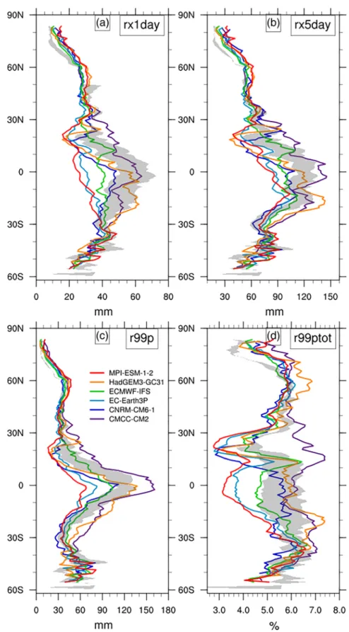
3.2. Model Evaluation
Wefirst evaluate the LR simulations of each model with regard to the zonal mean of their climatologies in precipitation extremes (over the 1985–2014 period). To that end, we compare the simulations to the observa-tional range (Figure 3). Some common features emerge from the results obtained for the four indices. First, the observational range is generally smaller than the intermodel differences in the mid‐to‐high latitude regions of the Northern Hemisphere (Figure 3). In the tropics, the observational range is also generally smal-ler than the intermodel differences despite relatively higher observational uncertainties in the tropics com-pared to the extratropics. In the Southern Hemisphere extratropics, zonal means of both observed and simulated climatological extreme precipitation are noisy due to a limited fraction of land; however, the range of observations and that of models seem to be of about the same magnitude. This seems to be also the case in the sub‐tropics for rx5day (Figure 3b). These results are generally in line with previous literature showing that the spread of ensembles of global (e.g., Herold et al., 2016) or regional (e.g. Prein & Gobiet, 2017) models can be of similar order of magnitude to the spread across different observations.
Figure 2. Maps show the multiproduct mean climatology (over the 1985–2014 period) of observed extreme precipitation indices for (a) rx1day, (b) rx5day, (c) r99p,
and (d) r99ptot. Vertical lines on the right‐hand side of each map refer to the zonal mean of the indices climatology in each of the three observational products: (black) REGEN, (gold) CPC, (brown) CHIRPS. CHIRPS does not provide data north of 50°N and south of 50°S (horizontal dashed red lines on maps), and therefore only the two in situ‐based data sets are averaged in the high latitudes. Horizontal black dashed lines indicate 25°S and 25°N, consistently referred to as the limit between the tropics and the extratropics in this study.
Figure 3. Zonal mean of climatological (over the 1985–2014 period) extreme precipitation indices in LR simulations
(colored lines, see inserted legend): (a) rx1day, (b) rx5day, (c) r99p, and (d) r99ptot. Gray shading illustrates the observational range defined by the zonal mean minimum and maximum values across the three observational products (REGEN, CPC, CHIRPS). CHIRPS does not provide data north of 50°N and south of 50°S, and therefore only the two in situ‐based data sets are considered in the high latitudes.
North of 60°N, all simulations are characterized by a wet bias for all indices (Figure 3). Wefind the best gen-eral agreement between observations and models between 30°N and 60°N, and this consistently for all four indices. Results are noisy in the Southern Hemisphere extratropics. In the tropics, most of the models simu-late smaller precipitation extremes compared to observations. The two models with the highest estimates of precipitation extremes (i.e., CMCC‐CM2 and HadGEM3‐GC31, which are coincidentally—or not—the two models of the ensemble with grid point dynamical cores, see Table 1 and section 4) are the closest to being consistent with observations in the tropics although not systematically. The four other models are generally drier than observations, and in particular, MPI‐ESM‐1‐2 and EC‐Earth3P compared to ECMWF‐IFS and CNRM‐CM6‐1. Overall, the LR simulations of the six models used here present limited agreement with observations for climatological precipitation extremes.
3.3. Impact of Increasing Horizontal Resolution
A major objective of this study is to assess the influence of an increase in atmospheric horizontal resolution for the simulation of precipitation extremes in global climate models. First, we note that the two models showing the smallest extremes in LR simulations in Figure 3 do not have the coarsest nominal resolutions of the multimodel ensembles (100 km for both MPI‐ESM 1‐2 and EC‐Earth3P compared to a range of 50 to 250 km for the ensemble; see Table 1). On the contrary, HadGEM3‐GC31, characterized by strong preci-pitation extremes, has the coarsest resolution of LR simulations across the ensemble of models, along with CNRM‐CM6‐1. Hence, the intermodel differences in nominal resolution do not help to explain the intermo-del spread in zonally averaged climatological precipitation extremes.
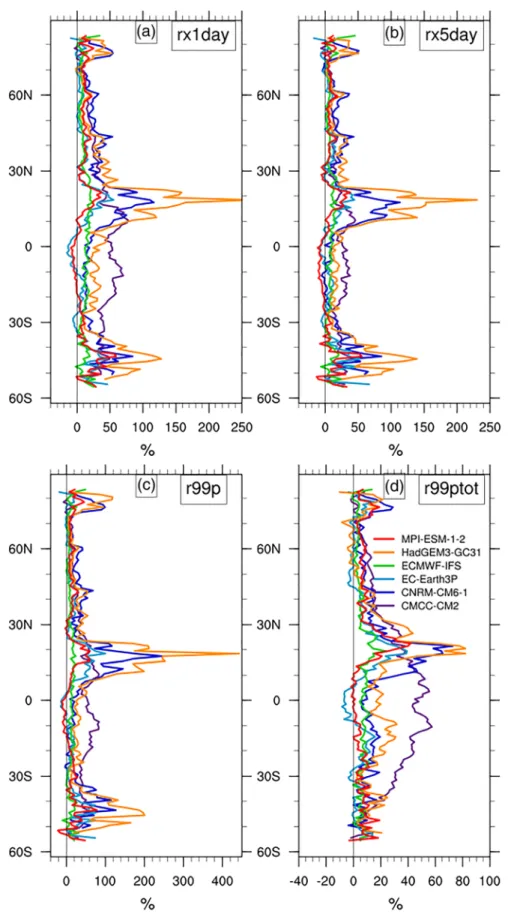
We then focus on the relative difference between the HR and LR simulations in the zonal mean of climato-logical precipitation extremes (over the 1985–2014 period; Figure 4) for each individual model. A common feature emerges from zonal means, with an intensification of precipitation extremes at higher resolution. Indeed, over most latitudes, for the great majority of models and for the four indices, HR simulations present an increase in precipitation extremes. This increase is often stronger in the tropics compared to the midlati-tudes. These results are consistent across the four indices; however, with larger intermodel differences for r99p and for the higher latitudes where results are noisier (Figure 4). Two models (CNRM‐CM6‐1 and HadGEM3‐GC31) show a very strong increase in precipitation extremes and in particular for r99p between 10°N and 23°N. The LR versions of these models underestimate r99p in this region, characterized by a mini-mum in this index (Figure 3).
Although there might be an intermodel relationship between the ratio of increase between the LR and HR resolution and the magnitude of intensification, it is not very clear. Indeed, MPI‐ESM‐1‐2, ECMWF‐IFS, and EC‐Earth3P share a similar and moderate ratio of grid refinement (i.e., 1:2 based on nominal resolutions; see Table 1) and often show the smallest intensification with increasing resolution, while HadGEM3‐GC31, CNRM‐CM6‐1, and CMCC‐CM2 have larger ratios of grid refinement (i.e., 1:5, 1:5, and 1:4, respectively) and can present higher intensifications. However, this is not always true for all indices and all latitudes, and the CNRM‐CM6‐1 response to increasing resolution is somehow different to HadGEM3‐GC31 and CMCC‐CM2. It is therefore difficult to extract such a relationship with confidence.
We further analyze the influence of higher resolutions in each individual model by analyzing the spatial dis-tribution of the relative difference between HR and LR simulations (Figure 5). While we see many regions associated with an intensification (blue colors), we can also find areas associated with a decrease in precipi-tation extremes at higher resolutions (red colors) for any of the four indices, and in any of the individual model. However, these regions are usually smaller in size and magnitude than regions of intensification, and there is no agreement across models on where these regions are. Note that internal variability might accentuate this lack of spatial agreement.
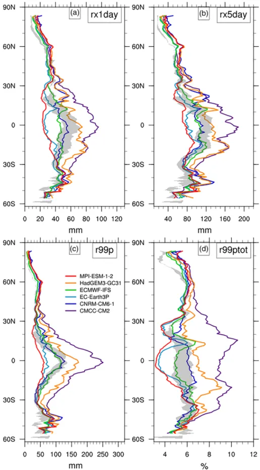
It remains to be understood if this general intensification of precipitation extremes at higher resolution leads to a better agreement with observations, and in particular over the tropics where extremes in the LR simula-tions are generally underestimated. As in Figure 3 for the LR simulasimula-tions, we compare the zonal means of climatological precipitation extremes in the HR simulations with the observations (Figure 6; note that differ-ent X‐axis ranges are used compared to Figure 3). In the tropics, we find that the two models with the highest estimates of precipitation extremes in their LR simulations (i.e., CMCC‐CM2 and HadGEM3‐GC31; Figure 3) overestimate extremes in their HR simulations, as they show an intensification of precipitation
Figure 4. Relative difference (%) between the HR and LR simulation of each model (colored lines, see inserted legend) in
the zonal mean of climatological (over the 1985–2014 period) extreme precipitation indices: (a) rx1day, (b) rx5day, (c) r99p, and (d) r99ptot.
extremes at higher resolution (Figure 4). On the other hand, MPI‐ESM‐1‐2 and EC‐Earth3P have among the driest estimates of precipitation extremes in their LR simulations compared to observations and the smallest intensification at higher resolution, which leads to an overall underestimation of precipitation extremes in their HR simulations. The HR simulations of the remaining two models (i.e., CNRM‐CM6‐1 and ECMWF‐IFS) generally sit within the observational range, which suggests an improvement with increasing resolution. However, we should remember that observational uncertainties are particularly large in the tropics.
North of 60°N, compared with the observations, precipitation extremes are overestimated in the LR simula-tions (Figure 3), and this is slightly amplified in the HR simulations (Figure 6), but as displayed in Figure 4, the intensification of precipitation extremes with resolution is generally lower than in the tropics. It is again difficult to find a consistent conclusion across the four indices in the case of the Southern Hemisphere
Figure 5. Relative differences (%) between HR and LR simulations in climatology (over the 1985–2014 period) of four extreme precipitation indices (per column;
see inserted legends) and for six models (per row; see inserted legends). Numbers in the bottom box indicate minimum and maximum values of relative difference over the globe. White areas are missing values and reflect that over dry regions the calculation of the 99th percentile was not robust because of too few wet days (see section 2.1). Horizontal black dashed lines indicate 25°S and 25°N, consistently referred to as the limit between the tropics and the extratropics in this study.
extratropics because of zonal mean variations but the intensification of precipitation extremes with resolu-tion seems to lead to an overestimaresolu-tion at higher resoluresolu-tion compared to observaresolu-tions (Figure 6).
In summary, our analysis generally indicates a simulated intensification of precipitation extremes at higher resolution, for all four indices. A clear message emerging from the analysis of Figure 6 (compared with Figure 3) is that we do not generally see better agreement with observations at higher resolutions for all mod-els. Indeed, zonal means of climatological extreme precipitation in both LR and HR simulations are gener-ally outside the range of observations over all latitudes, even if some simulations might be included in the observational range over some latitudes (e.g., HR simulations of ECMWF‐IFS and CNRM‐CM6‐1). It seems that the influence of horizontal resolution on precipitation extremes and its implications for agreement with observations is not straightforward, and we further investigate this by assessing model skill in the next section.
3.4. Model Skill
In this section, we evaluate the performance of the models in simulating precipitation extremes using the Arcsin‐Mielke M score (see section 2.4). The use of this metric allows further evaluation of model agreement with observations by measuring similarity in terms of intensity and spatial distribution. We measure the agreement between each model simulation and each observational product as a function of the nominal resolution (Figure 7). This skill score is calculated for climatologies (over the 1985–2014 period) for the four precipitation extreme indices over different terrestrial domains (latitudinal bands).
First, we note a large spread in the skill scores among models, across all the considered domains and indices. Wefind scores close to zero (close to no skill; see section 2.4) and scores greater than 700 (compared with a perfect agreement of 1,000). Such high scores (e.g., for rx1day, rx5day, and r99p in some regions for ECMWF‐IFS and EC‐Earth3P to a lesser extent) are similar to the scores obtained for mean seasonal preci-pitation by the best previous generation global climate models (IPCC, 2007; Meehl, 2007; Watterson et al., 2014). This emphasizes the fact that some new generation climate models, such as ECMWF‐IFS, pro-vide a generally good representation of extreme precipitation.
The skill scores can be very sensitive to the choice of the observation data set in some cases. For instance, for r99ptot in the tropics (Figure 7j), differences in skill scores for the LR simulations of HadGEM3‐GC31 are as large as 200 points between the three different data sets. Observational uncertainties are also assessed using the mean M score across each possible combination of two observational data sets (horizontal lines on panels, Figure 7). Similarity scores for observations can sometimes be very low (e.g., close to 400 for the extratropical regions of the Southern Hemisphere or the tropics for r99ptot; Figure 7l). The best agreement between observational data sets is noted for rx1day and r99p in the Northern Hemisphere extratropics and rx5day over all three domains, with mean observational M scores of ~750 (Figure 7). In a few cases, often involving the ECMWF‐IFS model, the agreement between models and observations is as good or even better than the mean agreement between observational data sets. These results clearly illustrate the challenge that exists in providing an accurate characterization of extreme precipitation in observations and the associated difficulty for model evaluation.
Despite large observational uncertainties, some robust conclusions still emerge from the analysis of Figure 7. The increase in resolution for a given model often does not lead to an improvement in the representation of precipitation extremes. The slopes of the lines that connect the skill scores at different resolutions are even often positive, meaning higher skill with lower horizontal resolution. This is particularly the case for MPI‐ESM 1‐2 and CMCC‐CM2 in the tropics. Obviously, these results are valid under the implicit hypothesis that there is no general underestimation of precipitation extremes across the three observation data sets. A systematic underestimation would indeed artificially result in higher skill scores for lower resolution mod-els, as their precipitation extremes have generally lower intensity compared to higher resolution versions of the models (Figure 6).
Additionally, there is little intermodel relationship between the skill of a model and its nominal resolution. CNRM‐CM6‐1 (together with HadGEM3‐GC31) is the model with the coarsest nominal resolution in its LR version but often has higher skill scores than higher resolution models. This shows that even if resolution has a clear impact on the simulation of precipitation extremes, other characteristics of atmospheric models play an even more important role, such as, very likely, the parameterization of convection.
Figure 7. Arcsin‐Mielke skill score for the four extreme precipitation indices (a–c: rx1day; d–f: rx5day; g–i: r99p; j–l: r99ptot) as a function of the model nominal
resolution. The score is computed over land for (left column) the tropics (25°S–25°N), (middle column) the midlatitude and high latitude of the Northern Hemisphere (25°N–90°N) and (right column) the mid latitude and high latitude of the Southern Hemisphere (25°S–60°S). HR and LR simulations of each model (see inserted color‐code on panel b) are evaluated to three different observational data sets in the tropics (CPC, REGEN and CHIRPS; see symbol‐code on panel a), and two data sets in the extratropics (CHIRPS is not used as it is limited to 50°S–50°N). Horizontal lines on each panel correspond to the average Arcsin‐Mielke skill score across all combinations of pair of observational products and are used as an estimate for observational uncertainty.
Note that uncertainties related to internal variability are much lower than the intermodel differences or the impact of observational uncertainties. Indeed, based on an ensemble of 10 realizations from the CNRM‐ CM6‐1 model, we measure the intramodel spread in M defined by the range in skill score across all realiza-tions (not shown). In the tropics and in Northern Hemisphere extratropics, internal variability in CNRM‐ CM6‐1 generally explains a spread in skill score smaller than 50, which is much smaller than both intermo-del and observational uncertainties. The largest intramointermo-del ranges for CNRM‐CM6‐1 in skill score are for r99ptot in the Southern Hemisphere extratropics, but they are generally smaller than 100, compared with intermodel spread close to 300.
3.5. Trends
The large impact of model resolution on climatological extreme precipitation raises the question of whether such an impact also exists with respect to the trends. We test how resolution influences the trends in preci-pitation extremes over a recent period (i.e., 1985‐2014, relatively short because of the availability of observa-tions), and we compare simulated and observed trends.
Our results do not indicate any clear sensitivity to spatial resolution across the four indices and the three ter-restrial domains of interest in this study (i.e., latitudinal bands; Figure 8). Indeed, we generallyfind similar trend values between the HR and LR simulations of each model, with the exception of the Southern Hemisphere extratropics (Figure 8, right column) where trends are mostly nonsignificant and where the intermodel spread is larger than in the other two domains. This is in general agreement with previous studies showing that resolution does not play a major role in explaining the different trends in large ensembles of models (e.g., Alexander & Arblaster, 2017 over Australia). Models agree best in the Northern Hemisphere extratropics (Figure 8, middle column), with positive and mostly significant trends, whereas there are larger differences from model to model in the tropics (Figure 8, left column) where trends are generally also posi-tive. Interestingly, in the tropics and for some indices in the Northern Hemisphere extratropics, wefind lar-ger differences in trend values among observations (black dots) than in models (colored dots in Figure 8) even if, overall, observations and models tend to agree on an increase in precipitation extremes over the recent decades.
4. Discussion
The previous results are likely dependent on the resolution of the grid used to compare observations and models after interpolation of daily precipitation. We chose to work on the moderate resolution grid (1° × 1°) of the FROGS observational database. This resolution is coarser than the resolution of the higher resolution models used in our study. It is therefore possible that the benefits of higher resolution would have been more obvious with a comparison to observations on afiner grid. However, this is not guaranteed, as we found large‐scale errors in higher resolution models, which would likely still exist on a finer comparison grid. Note also that Herold et al. (2017) show that observational uncertainties tend to be larger at higher reso-lutions. Also, even if some products with very high resolution exist, the effective resolution may be different in practice as in some regions the density of observations may be far too small to provide an adequate repre-sentation of spatial variations at these scales. Comparing models and observations at a higher resolution is therefore likely even more challenging.
We focus on forced‐atmospheric simulations and therefore we do not characterize impacts of increasing spa-tial resolution on precipitation extremes in a coupled framework. From a similar PRIMAVERA multimodel ensemble of coupled simulations, Vannière et al. (2019) found a more realistic representation of the mean ocean and atmosphere circulation at higher resolution compared to lower resolution coupled models and it remains to be assessed what this means for the potential impacts for precipitation extremes.
In a context of risk assessment, it is meaningful to focus on precipitation extremes over land only since this is where the majority of the impacts (such asflooding) occur. There are fewer satellite‐based observational pro-ducts that also cover the oceans (e.g., CHIRPS does not) and those which do are relatively short in time which prevent us from conducting our analyses over the oceans. Interestingly, it has been shown that increasing spatial resolution in models tends to bring more average precipitation globally, but with a con-trast in distributions over land and the oceans. Indeed, this global increase is partitioned into an increase over land and a decrease over the oceans, and this is explained by the enhanced large‐scale transport of
atmospheric moisture from the oceans to the land (Demory et al., 2014; Vannière et al., 2019). Similarly to Figure 4, we investigate the relative difference between the HR and LR simulations for precipitation extremes over the oceans. An overall intensification at higher resolution across all indices and all models is noted (Figure 9). The results are actually quite similar to those over land, with in particular HadGEM3‐GC31 and CMCC‐CM2 that generally show the greater intensification of extremes with resolution. It remains to be assessed whether the increase in precipitation extremes over the oceans leads to a better representation of precipitation extremes at higher resolutions. In a similar PRIMAVERA multimodel framework, M. J. Roberts et al. (2018) found that extratropical cyclones, a substantial source of extreme precipitation in the midlatitudes, are better represented in higher resolution simulations. Overall, there is a need for a systematic evaluation, in a multimodel framework, of the influence of higher resolution on precipitation extremes over the ocean.
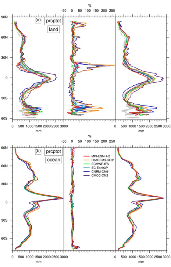
The comparison of results from Vannière et al. (2019) and our Figure 9 tend to show that over the oceans, mean, and extreme precipitation respond differently to increasing resolution in global climate models. This is confirmed in Figure 10, and it is also generally true over land. While we also find an intensification of annual total wet‐day precipitation (prcptot; see section 2.1) over both land and sea (middle panels of
Figure 8. Trends (mm per decade for a–i and % per decade for j–l) over 1985–2014 in extreme precipitation indices (per row; see inserted legends) averaged over
land in (left column) the tropics (25°S–25°N), (middle column) the Northern Hemisphere extratropics (25°N–90°N) and (right column) the Southern Hemisphere extratropics (25°S‐60°S). Black dots refer to observations and colored dots to models (see labels on X‐axis), with HR simulations indicated by a “H” in the middle of the dot. Significant (non‐significant) trends are represented by a filled dot (open circle). More details on the calculation of trends can be found in section 2.6. CHIRPS does not provide data north of 50°N and south of 50°S, and therefore only the two in situ‐based data sets are considered in the extratropics.
Figure 10. Left‐hand side and right‐hand side figure in each panel: Zonal mean of climatological (over the 1985–2014
period) prcptot in LR and HR (left and right, respectively) simulations (colored lines, see inserted legend) over (a) land and (b) oceans. Gray shading in (a) illustrates the observational range defined by the zonal mean minimum and maximum values across the three observational products (REGEN, CPC, CHIRPS). CHIRPS does not provide data north of 50°N and south of 50°S, and therefore only the two in situ‐based data sets are considered in the high latitudes. Middle figure in each panel: relative difference (%) between the HR and LR simulations of each model (colored lines, see inserted legend) in the zonal mean of climatological (over the 1985–2014 period) prcptot.
Figures 10a and 10b, respectively), this intensification is generally smaller compared to extreme precipita-tion (Figures 4 and 9). The large intensificaprecipita-tion of precipitaprecipita-tion extremes with resoluprecipita-tion noted previously seems therefore specific to the distribution tail. Furthermore, over land and for the zonal average of mean precipitation, all the models (in their LR and HR versions) are generally closer to the observations (left‐ and right‐hand side of Figure 10a) compared to extreme precipitation indices (Figures 3 and 6), despite the fact that observational uncertainties are considerably lower compared to extreme precipitation. No large overestimation is seen except for CMCC‐CM2 in the Tropics over land, at both resolutions.
Furthermore, in a similar PRIMAVERA multi‐model framework, Vannière et al. (2019) noted that the increase in global mean precipitation and the partitioning between land and ocean with increasing resolu-tion exhibits intermodel differences that could be partially explained by differences in the dynamical cores of the models (grid point versus spectral). In particular, they found stronger increase in mean precipitation over land by enhanced large‐scale moisture convergence in grid point models. Our results tend to be in line with this. Indeed, the two grid point models (i.e., HadGEM3‐GC31 and CMCC‐CM2, see Table 1) generally show the strongest intensification of extreme precipitation at higher resolution over land (Figure 4), yet interestingly over the oceans as well (Figure 9). The greater sensitivity of precipitation extremes to resolution over land in grid point models could be associated with a more realistic representation of orography in these models. The fact that precipitation extremes over ocean also show a greater intensification with resolution in grid point models suggests that the representation of orography is likely not the main cause. In any cases, it would be interesting to evaluate if there is a systematic relationship between this intensification at higher resolution and the dynamical cores of the models with a larger sample of models.
5. Conclusions
In this paper, we evaluate the representation of precipitation extremes over the 1985–2014 period in six new generation climate models within a forced‐atmospheric framework, focusing on four common indices (i.e., rx1day, rx5day, r99p, and r99ptot). We also assess the impact of higher atmospheric horizontal resolution on the simulation of precipitation extremes. Given the very large observational uncertainties for precipitation extremes (i.e., interproduct differences), which we illustrate in this study, three different observational data sets from different sources (i.e., in situ‐based and satellite‐based) are used.
For individual models, higher resolution generally leads to an intensification of precipitation extremes. This is in general agreement with previous studies based on experiments with a single model (e.g., Kopparla et al., 2013; Wehner et al., 2010, 2014 among others) or multimodel assessments at the regional scale from regional or global climate models (e.g., Caldwell, 2010; Giorgi et al., 2014; Rauscher et al., 2016; Scoccimarro et al., 2013, 2016). However, ourfindings show that quantitatively, and at the global scale, the intensification of precipitation extremes at increased resolution varies substantially from model to model.
The intensification of precipitation extremes at higher resolution does not necessarily lead to an improve-ment in skill. The skill of the models in simulating precipitation extremes is often lower at higher resolution. It could be because the protocol followed in the PRIMAVERA and HighResMIP projects recommends that the lower resolution version of the model is tuned and the same parameters are then kept at higher resolu-tion. This choice was made because modifying both the resolution and the parameters at the same time would not have allowed the characterization of solely the impact of resolution. However, extreme precipita-tion is generally not a metric that is directly assessed when performing the tuning of climate models. The main objective of the PRIMAVERA and HighResMIP projects is not to obtain the best‐possible high‐ resolution climate models, but to better characterize and understand the impact of resolution on the simu-lated climate. For precipitation extremes, it is likely that to fully benefit from running global climate models at higher resolution, dedicated work on adapting parametrization schemes to high resolution models is needed, most notably on the convection scheme.
Furthermore, there is no clear intermodel relationship between the skill in reproducing extreme precipita-tion and model nominal resoluprecipita-tion. Remarkably, the two models with the highest resoluprecipita-tion often span the best and worse skill scores of the ensemble. It is clear testimony that high resolution is not sufficient to improve the representation of precipitation extremes and that the dynamical core and/or physical para-meterizations also play a major role.
The clear sensitivity of precipitation extremes to horizontal resolution within individual models shows that high‐resolution global climate modeling presents a promising pathway to better meet the societal needs and the urgency for high resolution and high quality climate information for impact assessments. Nevertheless, in order for it to keep its promise, important model developments remain necessary. It would also be useful in a future study to analyze in details the physical processes (e.g., large scale versus convective precipitation, precipitation associated with frontal systems or tropical cyclones, orographic precipitation over steep terrain, etc.) associated with extreme precipitation in low‐ and high‐resolution models in order to gain a better understanding of why higher resolutions generally lead to more intense, and sometimes less realistic, preci-pitation extremes. Meanwhile, given the widely different skills of climate models in capturing extreme pre-cipitation, our study illustrates how a careful model selection might be necessary when dealing with precipitation extremes and their response to global warming that is largely uncertain over most regions of the globe (Bador et al., 2018; Collins et al., 2013; IPCC, 2013; Sillmann, Kharin, Zwiers, et al., 2013). The conclusions are generally and qualitatively robust to the choice of the observational data set, although some regional deviations are found. However, it should not mask the fact that observational uncertainties for precipitation extremes are substantial and should be considered with care. Our results on the impact of pre-cipitation uncertainties are in agreement with previous results from Wehner et al. (2014) who evaluated the ability of a single model to represent extreme precipitation at different spatial resolutions and concluded that the evaluation of the influence of high resolution was hindered by observational uncertainties, in particular in warm and poorly observed regions. Using an ensemble of global models, we show that the observational spread can be as large as the intermodel spread over global land. Observational uncertainties make the eva-luation of models and their adequate tuning very difficult, which highlights the need to pursue the effort on the estimation of observed precipitation extremes and the assessment of the differences among data sets. Data Availability Statement
The data that support thefindings of this study are openly available at:
FROGS observations: https://doi.org/10.14768/06337394-73A9-407C-9997-0E380DAC5598 CM2‐HR4: https://doi.org/10.22033/ESGF/CMIP6.1359
CM2‐VHR4: https://doi.org/10.22033/ESGF/CMIP6.1367 HadGEM3‐GC31‐LL: http://doi.org/10.22033/ESGF/CMIP6.1901 HadGEM3‐GC31‐HM: http://doi.org/10.22033/ESGF/CMIP6.446 MPI‐ESM 1‐2‐HR: https://doi.org/10.22033/ESGF/CMIP6.762 MPI‐ESM 1‐2‐XR:https://doi.org/10.22033/ESGF/CMIP6.10290 EC‐Earth3P: https://doi.org/10.22033/ESGF/CMIP6.2322 EC‐Earth3P‐HR: https://doi.org/10.22033/ESGF/CMIP6.2323 CNRM‐CM6‐1: https://doi.org/10.22033/ESGF/CMIP6.1925 CNRM‐CM6‐1‐HR: https://doi.org/10.22033/ESGF/CMIP6.1387 ECMWF‐IFS‐LR: http://doi.org/10.22033/ESGF/CMIP6.2463 ECMWF‐IFS‐HR: http://doi.org/10.22033/ESGF/CMIP6.2461
References
Alexander, L, & Herold, N (2015). ClimPACTv2 indices and software. A document prepared on behalf of the commission for climatology (CCl) expert team on sector‐specific climate indices (ET‐SCI).
Alexander, L. V., & Arblaster, J. M. (2017). Historical and projected trends in temperature and precipitation extremes in Australia in observations and CMIP5. Weather and Climate Extremes, 15(October 2016), 34–56. http://doi.org/10.1016/j.wace.2017.02.001 Alexander, L. V., Bador, M., Roca, R., Contractor, S., Donat, M., & Nguyen, P. (2020). Intercomparison of annual precipitation indices and
extremes over global land areas from in situ, space‐based and reanalysis products. Environmental Research Letters, 15(5), 055002. https:// doi.org/10.1088/1748-9326/ab79e2
Alexander, L. V., Fowler, H. J., Bador, M., Behrangi, A., Donat, M., Dunn, R., et al. (2019). On the use of indices to study extreme preci-pitation on sub‐daily and daily timescales. Environmental Research Letters, 14(12), 125008. https://doi.org/10.1088/1748-9326/ab51b6 Bador, M., Alexander, L. V, Contractor, S., & Roca, R. (2020). Diverse estimates of annual maxima daily precipitation in 22 state‐of‐the‐art
quasi‐global land observation datasets. Environmental Research Letters, 15(3), 35005. http://doi.org/10.1088/1748-9326/ab6a22
Acknowledgments
The PRIMAVERA project is funded by the European Union's Horizon 2020 Programme, grant agreement no. 641727. MB and LVA were supported by the Australian Research Council (ARC) Centre of Excellence for Climate Extremes (CE170100023). All analyses and graphics have been done using the NCAR Command Language (NCL 2013).
Bador, M., Donat, M. G., Geoffroy, O., & Alexander, L. V. (2018). Assessing the robustness of future extreme precipitation intensification in the CMIP5 ensemble. Journal of Climate, 31(16), 6505–6525. http://doi.org/10.1175/JCLI-D-17-0683.1
Caldwell, P. (2010). California wintertime precipitation bias in regional and global climate models. Journal of Applied Meteorology and
Climatology, 49(10), 2147–2158. https://doi.org/10.1175/2010JAMC2388.1
Chen, C.‐T., & Knutson, T. (2008). On the verification and comparison of extreme precipitation indices from climate models. Journal of
Climate, 21(7), 1605–1621. https://doi.org/10.1175/2007JCLI1494.1
Cherchi, A., Fogli, P. G., Lovato, T., Peano, D., Iovino, D., Gualdi, S., et al. (2019). Global mean climate and main patterns of variability in the CMCC‐CM2 coupled model. Journal of Advances in Modeling Earth Systems, 11, 185–209. https://doi.org/10.1029/ 2018MS001369
Collins, M., & Coauthors (2013). Long‐term climate change: Projections, commitments and irreversibility. In T. F. Stocker, et al. (Eds.),
Climate Change 2013: The Physical Science Basis(pp. 1029–1136). Cambridge: Cambridge University Press.
Contractor, S., Donat, M. G., Alexander, L. V., Ziese, M., Meyer‐Christoffer, A., Schneider, U., et al. (2020). Precipitation estimates on a gridded network (REGEN)—A global land‐based gridded dataset of daily precipitation from 1950–2013, Hydrol. Earth Syst. Sci. Discuss,
24(2), 919–943. https://doi.org/10.5194/hess-24-919-2020
Demory, M. E., Vidale, P. L., Roberts, M. J., Berrisford, P., Strachan, J., Schiemann, R., & Mizielinski, M. S. (2014). The role of horizontal resolution in simulating drivers of the global hydrological cycle. Climate Dynamics, 42(7–8), 2201–2225. http://doi.org/10.1007/s00382-013-1924-4
Donat, M. G., Alexander, L. V., Herold, N., & Dittus, A. J. (2016). Temperature and precipitation extremes in century‐long gridded observations, reanalyses, and atmospheric model simulations. Journal of Geophysical Research: Atmospheres, 121, 11,174–11,189. https://doi.org/10.1002/2016JD025480
Donat, M. G., Sillmann, J., Wild, S., Alexander, L. V, Lippmann, T., & Zwiers, F. W. (2014). Consistency of temperature and precipitation extremes across various global gridded in situ and reanalysis datasets. Journal of Climate, 27(13), 5019–5035. http://doi.org/10.1175/ JCLI-D-13-00405.1
Eyring, V., Bony, S., Meehl, G. A., Senior, C. A., Stevens, B., Stouffer, R. J., & Taylor, K. E. (2016). Overview of the coupled model inter-comparison project phase 6 (CMIP6) experimental design and organization. Geoscientific Model Development, 8(12), 10,539–10,583.
https://doi.org/10.5194/gmdd-8-10539-2015
Flato, G., Marotzke, J., Abiodun, B., Braconnot, P., Chou, S. C., Collins, W., et al. (2013). Evaluation of climate models. Climate change 2013: The physical science basis. Contribution of Working Group I to the Fifth Assessment Report of the Intergovernmental Panel on
Climate Change, 741–866. http://doi.org/10.1017/CBO9781107415324.020
Funk, C., Peterson, P., Landsfeld, M., Pedreros, D., Verdin, J., Shukla, S., et al. (2015). The climate hazards infrared precipitation with stations—A new environmental record for monitoring extremes. Scientific Data, 2, 1–21. https://doi.org/10.1038/sdata.2015.66 Gervais, M., Tremblay, L. B., Gyakum, J. R., & Atallah, E. (2014). Representing extremes in a daily gridded precipitation analysis over the
United States: Impacts of station density, resolution, and gridding methods. Journal of Climate, 27(14), 5201–5218. http://doi.org/ 10.1175/JCLI-D-13-00319.1
Giorgi, F., Coppola, E., Raffaele, F., Diro, G. T., Fuentes‐Franco, R., Giuliani, G., et al. (2014). Changes in extremes and hydroclimatic regimes in the CREMA ensemble projections. Climatic Change, 125(1), 39–51. https://doi.org/10.1007/s10584-014-1117-0
Gleckler, P. J., Taylor, K. E., & Doutriaux, C. (2008). Performance metrics for climate models. Journal of Geophysical Research, 113, D06104. http://doi.org/10.1029/2007JD008972
Gutjahr, O., Putrasahan, D., Lohmann, K., Jungclaus, J. H., von Storch, J. S., Brüggemann, N., et al. (2019). Max Planck institute earth system model (MPI‐ESM 1.2) for high‐resolution model intercomparison project (HighResMIP). Geophysical Model Development, 12(7), 3241–3281. https://doi.org/10.5194/gmd-12-3241-2019
Haarsma, R., et al. (2020). HighResMIP versions of EC‐earth: EC‐Earth3P and EC‐Earth3P‐HR. description, model performance, data handling and validation. Geoscientific Model Development Discussion, 2020, 1–37.
Haarsma, R. J., Roberts, M. J., Vidale, P. L., Senior, C. A., Bellucci, A., Bao, Q., et al. (2016). High resolution model intercomparison project (HighResMIP v1. 0) for CMIP6. Geoscientific Model Development, 9(11), 4185–4208. https://doi.org/10.5194/gmd-9-4185-2016
Hennessy, K. J., Suppiah, R., & Page, C. M. (1999). Australian rainfall changes, 1910–1995. Australian Meteorological Magazine, 48, 1–3. Herold, N., Alexander, L. V., Donat, M. G., Contractor, S., & Becker, A. (2016). How much does it rain over land? Geophysical Research
Letters, 43, 341–348. http://doi.org/10.1002/2015GL066615
Herold, N., Behrangi, A., & Alexander, L. V. (2017). Large uncertainties in observed daily precipitation extremes over land. Journal of
Geophysical Research, 122, 668–681. http://doi.org/10.1002/2016JD025842
IPCC (2001). In J. T. Houghton, et al. (Eds.), Climate change 2001: The scientific basis: Contribution of Working Group I to the Third Assessment Report of the 145 References Intergovernmental Panel on Climate Change(p. 881). New York, NY: Cambridge University Press.
IPCC (2007). Climate change 2007—The physical science basis: Contribution of Working Group I to the Fourth Assessment Report of the IPCC, edited by Cambridge University Press et al., ISBN 978 0521 88009‐1 Hardback; 978 0521 70596‐7 Paperback, Cambridge Univ. Press, New York, NY
IPCC (2013). In T. F. Stocker, D. Qin, G.‐K. Plattner, M. Tignor, S. K. Allen, J. Boschung, A. Nauels, Y. Xia, V. Bex, & P. M. Midgley (Eds.),
Climate change 2013: The physical science basis. Contribution of Working Group I to the Fifth Assessment Report of the Intergovernmental Panel on Climate Change(p. 1535). Cambridge, UK, and New York, NY: Cambridge University Press. https://doi.org/10.1017/ CBO9781107415324
Kennedy, J., Titchner, H., Rayner, N., & Roberts, M. (2017). input4MIPs.MOHC.SSTsAndSeaIce.HighResMIP.MOHC‐HadISST‐2‐2‐0‐0‐0. Version 20170505. Earth system grid federation. https://doi.org/10.22033/ESGF/input4MIPs.1221
Kharin, V. V, Zwiers, F. W., Zhang, X., & Wehner, M. (2013). Changes in temperature and precipitation extremes in the CMIP5 ensemble.
Climatic Change, 119(2), 345–357. Article. https://doi.org/10.1007/s10584-013-0705-8
Kim, I. W., Oh, J., Woo, S., & Kripalani, R. H. (2019). Evaluation of precipitation extremes over the Asian domain: Observation and modelling studies. Climate Dynamics, 52(3–4), 1317–1342. http://doi.org/10.1007/s00382-018-4193-4
Kopparla, P., Fischer, E. M., Hannay, C., & Knutti, R. (2013). Improved simulation of extreme precipitation in a high‐resolution atmo-sphere model. Geophysical Research Letters, 40, 5803–5808. https://doi.org/10.1002/2013GL057866
Meehl, G. A., Stocker, T. F., Collins, W. D., Friedlingstein, P., Gaye, A. T., Gregory, J. M., Kitoh, A., et al. (2007). Global climate projections. In S. Solomon, D. Qin, M. Manning, Z. Chen, M. Marquis, K. B. Averyt, M. Tignor, & H. L. Miller (Eds.). Climate change 2007: The
physical science basis. Contribution of Working Group I to the Fourth Assessment Report of the Intergovernmental Panel on Climate Change. Cambridge University Press, Cambridge, UK, and New York, NY.