Application of fuzzy representation of geographic boundary to the soil loss model

(1)

HAL Id: hal-00298645

https://hal.archives-ouvertes.fr/hal-00298645

Submitted on 3 Feb 2006

HAL is a multi-disciplinary open access

archive for the deposit and dissemination of sci-entific research documents, whether they are pub-lished or not. The documents may come from teaching and research institutions in France or abroad, or from public or private research centers.

L’archive ouverte pluridisciplinaire HAL, est destinée au dépôt et à la diffusion de documents scientifiques de niveau recherche, publiés ou non, émanant des établissements d’enseignement et de recherche français ou étrangers, des laboratoires publics ou privés.

Application of fuzzy representation of geographic

boundary to the soil loss model

G.-S. Lee, K.-H. Lee

To cite this version:

G.-S. Lee, K.-H. Lee. Application of fuzzy representation of geographic boundary to the soil loss model. Hydrology and Earth System Sciences Discussions, European Geosciences Union, 2006, 3 (1), pp.115-133. �hal-00298645�

(2)

HESSD

3, 115–133, 2006

Application of fuzzy boundary G.-S. Lee and K.-H. Lee

Title Page Abstract Introduction Conclusions References Tables Figures J I J I Back Close

Full Screen / Esc

Print Version

Interactive Discussion

EGU

Hydrol. Earth Syst. Sci. Discuss., 3, 115–133, 2006 www.copernicus.org/EGU/hess/hessd/3/115/ SRef-ID: 1812-2116/hessd/2006-3-115 European Geosciences Union

Hydrology and Earth System Sciences Discussions

Papers published in Hydrology and Earth System Sciences Discussions are under open-access review for the journal Hydrology and Earth System Sciences

Application of fuzzy representation of

geographic boundary to the soil loss

model

G.-S. Lee and K.-H. Lee

Korea Water Resource Corporation, 462-1 Jeonmin-dong, Yusung-gu, Daejeon, Korea Received: 7 November 2005 – Accepted: 29 November 2005 – Published: 3 February 2006 Correspondence to: G.-S. Lee (ilovegod@kowaco.or.kr)

(3)

HESSD

3, 115–133, 2006

Full Screen / Esc

Print Version

EGU

Abstract

The polygon boundaries on the digital map of land surface characteristic are conven-tionally represented as a sharp change (categorical format), which results in discrep-ancy between real world phenomena and the information presented by boundaries on map, and it is especially true for soil properties. This paper presents a probable impact

5

of the representation of geographic boundary for the soil loss model. To do this, the Revise Universal Soil Loss Equation (RUSLE) model is facilitated at a small basin in Korea and then the fuzzy representation of geographic boundary, which is presumably better description of soil properties in nature, was introduced into the soil factors in the RUSLE. The model results were compared to the conventional representation of sharp

10

change in relative terms. The model results show the impact of the fuzzy representa-tion on the RUSLE model is considerable and the soil loss model is expected to use more realistic description for geographic boundaries of land surface characteristics. The method suggested herein is relatively simple and has wide applicability.

1. Introduction

15

Extremely heavy rainfall events over the last decade have been increasing, which has an effect on various aspects and, especially, soil loss has been a threat to farm liveli-hoods and ecosystem integrity. A soil loss modeling approach is widely used for pre-dicting water erosion hazards and planning of soil conservation measures. Soil loss models often require two main input data to estimate the amount of soil loss;

meteoro-20

logical forcing and surface characteristics description. The advancement of the remote sensing technique has been a great potential to surface characteristics description and the remotely sensed digital map is usually handled by Geographic Information system (GIS). The GIS skill may by far improve processing efficiency and accuracy in many aspects but still have some limitations in dealing with boundary information (Wang

25

(4)

HESSD

3, 115–133, 2006

Full Screen / Esc

Print Version

EGU

format and polygon boundaries delineate and thereby distinguish areas with different surface characteristics. Accordingly the polygon boundaries on the digital map are conventionally represented as a sharp change, which results in discrepancy between real world conditions and the information presented by boundaries on map (Burrough, 1986, 1992). Each zone with an abrupt line is a cadastral map where abrupt boundary

5

definition is required to differentiate land parcels that have unique property (Hunter and Williamson, 1990). It is especially true for soil properties because boundaries of soil properties are changing and rarely sharp or crisp in nature. In reality, localized partial change, gradual transition, and other non-sharp changes generally coexist in soil prop-erties (Burrough, 1986; Burrough and Andrew, 1986). From this perspective, Walsh

10

(1989) has suggested that soil boundaries should be more realistically described as zones of transition rather than abrupt change. Despite its importance, no much re-search has been performed to improve the expressive ability of polygon boundaries in soil loss modeling approach. In fact, the unrealistic description of geographic bound-aries may not cause serious problem in a visual way because human beings are

ca-15

pable of dealing with inaccuracy by using common sense, knowledge, and experience, while the computer cannot interpret a sharp change as anything else unless it is ex-plicitly programmed to do so (Wang and Hall, 1996).

The objective of the present study is to examine probable impact of the representa-tion of geographic boundary for soil loss generarepresenta-tion. To overcome the expressive

inad-20

equacy of geographic boundary, we introduced a fuzzy representation of geographic boundary, which is presumably better description of soil properties, to improve the esti-mation of soil loss generation. The fuzzy representation of geographic boundary is an advanced geographic boundary representation which enhances the expressive prop-erties of polygons and also improves the problem of misrepresentation of continuously

25

distributed phenomena created by use of sharp polygon boundaries where gradual or partial changes in thematic properties are likely to occur (Wang and Hall, 1996). There are six main factors to adequately represent all the surface characteristics in the RUSLE and the accuracy of estimation in soil loss generation highly depends in

(5)

HESSD

3, 115–133, 2006

Full Screen / Esc

Print Version

EGU

part on how well these model factors describe the relevant characteristics of the basin. Hence using the fuzzy representation of geographic boundary into the soil factors is a challenging and innovative for the estimation of soil loss generation.

The model results were compared to the conventional representation of sharp change in relative terms. The model results show the impact of the fuzzy

represen-5

tation on the RUSLE model is considerable and the method is expected to contribute to improve soil conservation measure.

In the following section we briefly described the procedure for the soil loss model set up, followed by basic theoretical background. In the fourth section we explicitly explained the application results of fuzzy representation of geographic boundary to

10

soil erodibility factor (K) in the RUSLE and we close the paper with summary and conclusions in the last section.

2. Soil loss model set up

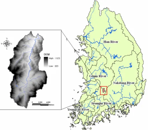
The RUSLE is facilitated at the Jang-gye basin, southern part of Geum river. The center of the basin is 127◦310E, 37◦400N, which is about 210 km south of the capital of

15

Korea (Fig. 1) and it covers about 116.46 km2and the elevation is in the range of 323– 1123 m. Its annual average temperature and humidity are approximately 13◦and 72%, respectively and its annual average precipitation (=1230 mm) is slightly lower than the Korean national average (=1283 mm).

In the RUSLE, there are six factors which describe the land surface characteristics

20

and meteorological conditions as mentioned earlier. The Toxopeus equation is well known for its superiority in Korea (KICT, 1992) and selected for calculating rainfall ero-sivity factor, R as follows;

R= 38.5 + 0.35 × Pr (1)

where R is rainfall erosivity factor (in MJ ·mm·ha−1·yr−1) and Pr is the annual average

25

(6)

HESSD

3, 115–133, 2006

Full Screen / Esc

Print Version

EGU

period of the year 1983–2002 and interpolated using spline method.

The K-factor reflects the ease with which the soil is detached by splash and surface flow. The K-factor varies with soil texture, organic matter content permeability, and other factors and then it is often transformed from the soil texture map (Wischmeier, 1971). Detailed procedure to derive the K-factor is described in later section.

5

The RUSLE describes topographic effect by means of the L- and S- factor, which accounts for the effect of slope length and slope gradient on erosion, respectively. A number of empirical equations for calculating the L and S factors have been suggested (McCool et al., 1989; Barsch, 1998; Yitayew et al., 1999) but the selection of a suitable algorithm is dependent on the characteristics of the particular basin and application.

10

Renard et al. (1991) used the number of grid cells flowing into the observation cell and the cell length as a multiplier to determine the total hillslope length of the segment. The cell-based method accounts for the divergence and convergence of flows and attempts to take into account the complexity of natural landscapes. Hence, the method of Renard et al. (1991) was selected as follows;

15

β= (sin θ/0.0896) (2.96 × sin0.79θ+ 0.56)

, m= β

(1+ β) (2)

where m is the slope length exponent and θ is the angle of slope.

L_i =x

m

(im+1− (i − 1)m+1)

22.13m (3)

where L_i is the slope length factor for the cell at ith segment and x is the length of the grid cell(m).

20

The algorithm of Nearing (1997) was used to calculate the slope steepness factor, S reflects.

S = −1.5 + 17

1+ exp(2.3 − 6.1 sin θ) (4)

(7)

HESSD

3, 115–133, 2006

Full Screen / Esc

Print Version

EGU

In the RUSLE, the C-factor reflects the abundance and type of the vegetation. The C-factor is dependent on the type of crop, the phenology, cultivation methods and man-aging factors (Dissmeyer and Foster, 1981; Gilley, 1986). The C-factor varies from near zero for well-protected land cover to 1 for barren area. The land cover map derived from the Landsat TM imagery is used to extract cover management factor, C.

5

The P-factor is a reflection of soil loss due to the flow pattern change, gradient, direction of surface runoff, and reduction of runoff rate resulting from variable cultivation (Renard and Foster, 1983). The cell-based representations of map features used in the RUSLE offer analytical capabilities for continuous data and allow fast processing of map layer (Fernandez et al., 2003). The mean annual gross soil erosion is calculated

10

on the cell basis using the combination of the product of six factors as follows;

A= R × K × L × S × C × P (5)

where A denotes the average soil loss due to water erosion (in ton·ha−1·yr−1). The L, S, C, and P are all dimensionless. The amount of soil loss generation is calculated on a yearly basis for the spatial resolution of 22 m in this study.

15

3. Theoretical background

As shown in Fig. 2, three different types of models are, in general, used to effec-tively represent geographic boundaries in GIS; abrupt change (Type I), large change (Type II), and gradual change (Type III) (Vincent, 1991; Wang and Hall, 1996).

The membership function of a set defines how the “grade of membership” of an

in-20

dividual with an attribute value of x is determined. The membership function converts attribute values x to membership function values (MF_x). For conventional crisp sets of the polygon boundaries on the digital map, the membership function can be

(8)

repre-HESSD

3, 115–133, 2006

Full Screen / Esc

Print Version Interactive Discussion EGU sented as follow; MF_x = 0 for x < b₁ MF_x = 1 for b₂≥ x ≥ b₁ MF_x = 0 for x > b₂ (6)

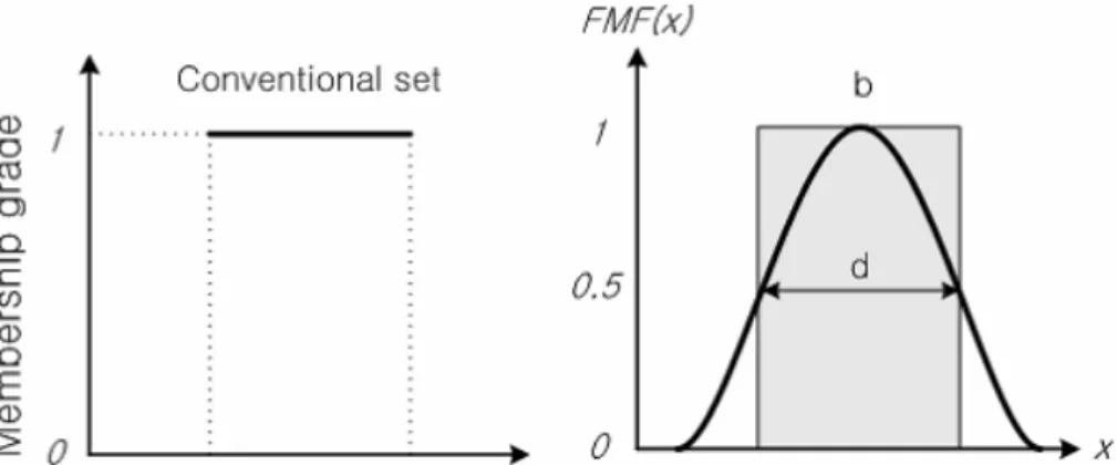
where b₁and b₂ define the exact upper and lower limits of the set. The left panel on Fig. 3 graphically shows the membership function of the conventional representation of geographic boundaries.

5

For fuzzy sets, the limits b₁, b₂define the central concept of the set. The fuzzy mem-bership function (FMF) defines how the possibility of memmem-bership varies continuously from 0 (for individuals that are completely outside the set) to 1 (for objects that within the central concept). The attribute value at the point where “the grade of membership=0.5” (see right panel on Fig. 3) is called the “crossover point” (Burrough, 1992).

10

Rather than the binary membership conditions of classic set theory (1 or 0), a fuzzy membership condition allows more realistic modeling of geographic properties with high spatial within-class variability, whereby membership grades accommodate the ex-treme classical case, as well as all other possibilities in between (Wang and Hall, 1996). Several functions can be selected to define flexible FMFs, which can be either

symmet-15

ric or asymmetric with regards to the central concept and the degree of dispersion. The following fuzzy classification models, which are suitable for soil property data, are an extension version of Kandel (1998). It is a simple model and a general symmetric bell-form FMF.

F MF_x = 1

[1+ {(x − b)/d}2_] for 0 ≤ x ≤ P

20

F MF_x = 1 for x > P (7)

The parameter b defines the value of the attributes x at the central concept of the standard index of the set. The form of the membership function and the position of the crossover points can be easily changed by changing the value of the dispersion index, d. The parameter d gives the width of the bell curve at the crossover point, which

(9)

HESSD

3, 115–133, 2006

Full Screen / Esc

Print Version

EGU

defines the transition zone around the central core of the set in the same units as the central concept. Equation (7) is selected for the FMF and the parameter b and d was identically given in this study. The right panel on Fig. 3 shows the shape of the FMF.

Detailed explanation of the fuzzy theory is beyond the scope of the study and the readers are referred to Burrough (1992) and Kandel (1998) for more details.

5

4. Application of fuzzy representation to soil erodibility factor, K

The central goal of the study is to investigate the probable impact of the representation of geographic boundary in soil erodibility factor, K in the RUSLE model. We focused on demonstrating the concept and methodology. To do this, we made two simulation scenarios; one is for the conventional representation of sharp change and the other is

10

for the fuzzy representation of within-class variability described in Eq. (7). Hence, the only source that would differentiate the amount of soil loss generation among the two simulation scenarios is the different description of geographic boundaries. In typical fashion, a value of soil erodibility factor, K is assigned for each grid cell (22 m) accord-ing to the soil type-soil erodibility conversion (see left panel on Fig. 3). Table 1 presents

15

assigned soil erodibility factors, K according to each soil type classification followed by KICT (1992). Each soil type has its own sand %, clay %, and silt % from the sampling test (KICT, 1992) and then, K-factors were retrieved from the Erickson’s triangle dia-gram (Erickson, 1997). Consequently the basin is divided into several patches that are homogeneous in terms of soil properties and it is called the conventional

representa-20

tion of sharp change (Type I in Fig. 2). Each soil patch is assigned one soil type (one K-factor) and is distinguished by another boundary of soil type. However, the K factor has different values depending in part on how to specify soil type in the RUSLE bound-ary cell and it can be explicitly controlled as mention earlier. To make the soil boundbound-ary of soil map more realistic, the simple FMF (Eq. 7 and right on Fig. 3) is then used and

25

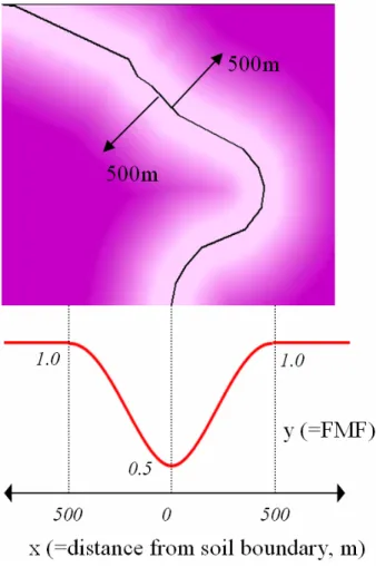
the image of Fig. 4 shows a detailed fuzzy-knowledge based boundary description with 500 m Euclidian distance. It is assumed that the Euclidian distance of 500 m is covered

(10)

HESSD

3, 115–133, 2006

Full Screen / Esc

Print Version

EGU

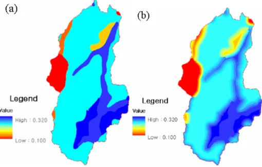
by the fuzzy representation from the boundary because soil samples were taken at every 1 km for soil map (Nisar Ahamed et al., 2000). In other words, the FMF to 500 m spacing on both directions of the soil boundary is considered to calculate soil erodibility factor, K as shown in Fig. 4. Figure 5a shows the 2-D imagery map for the soil erodi-bility, K of the conventional sharp change, while Fig. 5b shows the 2-D imagery map

5

for the soil erodibility, K as a result of the fuzzy representation. The fuzzy-knowledge based boundary in Fig. 5b (blurry area) is called the fuzzy representation of geographic boundary (Type II in Fig. 2) and then it is regarded as reproducing more real condition in relative terms. Table 2 presents basic statistics of the value of K-factor for both meth-ods. With the fuzzy representation, the mean value of the K-factors is slightly increased

10

and the standard deviation is decreased, while the maximum/minimum values are not changing.

The fuzzy representation is intended for improving the estimation of soil loss genera-tion and eventually predicting water erosion hazards and planning of soil conservagenera-tion measures. It is a main interest to see how the fuzzy representation has an influence on

15

the amount of soil loss generation in the modeling approach. Table 2 presents the anal-ysis results of annual soil loss simulated by the RUSLE for each method. The mean (standard deviation) of soil loss for the fuzzy representation is higher by 2.5 (2.3)% and the maximum value for the fuzzy representation is higher by 21%.

As shown in Eq. (5), the amount of soil loss is given as the combination of the

20

product of six factors. Then, soil loss change at the boundaries depends on the relative membership grade of the fuzzy function (Type II) comparing to that of the sharp change (Type I) because the remaining factors (R-, L-, S-, C-, and P-factor) are not changing. Consequently the fuzzy representation of geographic boundary in the RUSLE results in higher estimation of soil loss for the study basin.

25

The study area is a small basin with 116.46 km2 and it consists of a small number of different soil patches in relative terms. However, difference may be large for large basins because of its high spatial variability and larger portion of boundaries. Then, the results shown in this study may be different for every new basin of interest because

(11)

HESSD

3, 115–133, 2006

Full Screen / Esc

Print Version

EGU

the amount of soil loss is highly dependent on the selection of model, the quality of geospatial data, and the basin characteristics, but the method used herein should work anywhere.

5. Summary and conclusions

The digitalized soil texture map handled by GIS is used to describe real world

condi-5

tion, but has some limitations in the expressive ability in boundary information. The RUSLE model was facilitated at a small basin in Korea to investigate probable impact of the representation of geographic boundary for soil loss generation. A fuzzy repre-sentation of geographic boundary is presumably better description of soil properties in that it includes within-class variability concept, which can not be properly described by

10

membership in a single set of sharp change. The primary conclusions of the study are as follows;

– With the fuzzy representation, the mean value of the K-factors is slightly increased

and the standard deviation is decreased, while the maximum/minimum values are not changing.

15

– The mean (standard deviation) of soil loss for the fuzzy representation is higher

by 2.5 (2.3) (in %) and the maximum value for the fuzzy representation is higher by 21 (in %).

– Consequently the fuzzy representation of geographic boundary in the RUSLE

results in higher estimation of soil loss in the study basin.

20

– The results shown in this study may be different for every new basin of interest,

but the method used herein should work anywhere.

On the basis of the results, soil loss estimation depends in part on how to describe the surface boundary in the modeling approach. The approach suggested herein has wide

(12)

HESSD

3, 115–133, 2006

Full Screen / Esc

Print Version

EGU

applicability and can be extended to any land surface model concerning soil properties. More realistic description of geographic boundary such as the fuzzy representation is desirable in dealing with soil properties of the soil loss model.

Acknowledgements. This study was supported by Korea Water Resources Corporation project # KIWE-CHR-04-4.

5

References

Bartsch, P.: Modelling Soil Loss to determine water erosion risk at Camp Williams national guard base, Ph.D. Dissertation, UTAH State University, 1998.

Burrough, P. A.: Fuzzy classification methods for determining land suitability from soil profile observations and topography, J. Soil Sci., 43, 193–210, 1992.

10

Burrough, P. A.: Principles of geographical information systems for land resource assessment, Clarenden Press, Oxford, UK, 1986.

Burrough, P. A. and Frank, A. U.: Geographic Objects with Indeterminate Boundaries, Taylor & Francis, p. 3–28, 1996.

Dissmeyer, G. E. and Foster, G. R.: Estimating the cover management factor in the USLE for

15

forest conditions, J. Soil Water Conservation, 36(4), 235–240, 1981.

Erickson, A. J.: Aids for estimating soil erodibility – K value class and soil loss tolerance, U.S. Department of Agriculture, Soil Conservation Services, Salt Lake City of Utah, 1997. Fernandez, C., Wu, J. Q., McCool, D. K., and Stockle, C. O.: Estimating water erosion and

sed-iment yield with GIS, RUSLE, and SEDD; J. Soil Water Conservation, 58, 128–136, 2003.

20

Gilley, J. E., Finkner, S. C., Spomer, R. G., and Mielke, L. N.: Runoff and erosion as affected by crop, Trans. Amer. Assoc. Agricultural Eng., 29(1), 157–160, 1986.

Hunter, G. J. and Williamson, I. P.: The development of a historical digital cadastral database, Int. J. Geographic Information Systems, 4, 169–180, 1990.

Kandel, A.: Fuzzy Mathematical Techniques with Applications, Addison-Wesley, Reading, MA,

25

1998.

Korea Institute of Construction Technology (KICT): The development of selection standard for calculation method of unit sediment yield in river, KICT 89-WR-113 Research Paper (In Ko-rean), 1992.

(13)

HESSD

3, 115–133, 2006

Full Screen / Esc

Print Version

EGU

McCool, D. K., Foster, G. R., Mutchler, C. K., and Meyer, L. D.: Revised Slope Length Factor the Universal Soil Loss Equation, Trans. Amer. Soc. Agricultural Eng., 32(5), 1571–1576, 1989.

Nearing, M. A.: A single continuous function for slope steepness influence on soil loss, Soil Sci. Soc. Amer. J., 61(3), 917–919, 1997.

5

Nisar Ahamed, T. R., Gopal Rao, K., and Murthy, J. S. R.: Fuzzy class membership approach to soil loss modeling, Agricultural Systems, 63, 97–110, 2000.

Renard, K. G. and Foster, G. R.: Soil Conservation-Principles of erosion by water, in: Dryland Agriculture, American Society of Agronomy, edited by: Dregne, H. E. and Willies, W. O., Soil Sci. Soc. Amer., Madison, WO, USA, 155–176, 1983.

10

Renard, K. G, Foster, G. R., Weesies, G. A., and Porter, P. J.: RUSLE: Revised Universal Soil Loss Equation, J. Soil Water Conservation, 46(1), 30–33, 1991.

Vincent, P.: Modeling binary maps using ARC/INFO and GLIM, in: Proceedings of the Euro-pean Conference on Geographic Information Systems (EGIS 90), (Utrecht: EGIS Founda-tion), 1108–1116, 1991.

15

Walsh, S. J.: User considerations in landscape characterization, in: The accuracy of spatial databases, Taylor and Francis, London, UK, 35–44, 1989.

Wang, F. and Hall, G. B.: Fuzzy representation of geographical boundaries in GIS, Int. J. Geo-graphic Information System, 10(5), 573–590, 1996.

Wischmeier, W. H.: A Soil Erodibility Nomograph for Farmland and Construction sites, J. Soil

20

Water Conservation, 26, 189–193, 1971.

Yitayew, M., Pokrzywka, S. J., and Renard, K. G.: Using GIS for facilitating erosion estimation, Appl. Eng. Agric., 15, 295–301, 1999.

(14)

HESSD

3, 115–133, 2006

Full Screen / Esc

Print Version

EGU

Table 1. Assigned soil erodibility factor, K according to each soil type classification followed

by KICT (1992). Each soil type has its own sand %, clay %, and silt % from the sampling test (KICT, 1992). Then, K-factors were retrieved from the Erickson’s triangle diagram. The K factor has different values depending in part on how to represent soil type in the RUSLE boundary cell.

Soil Name Description K

Mangyeong coarse silty, mixed, nonacid, mesic family of Fluventic Haplaquepts 0.27 (Low Humic-Gley soils)

Mudeung fine loamy, mesic family of Lithic Dystrochrepts (Lithosols) 0.18

Mui coarse loamy, mixed, mesic family of Umbric Dystrochrepts (Regosols) 0.31

Manseong fine loamy over sandy skeletal, mixed, nonacid, mesic family of 0.20

Aeric Fluventic Haplaquepts (Low Humic-Gley Alluvial soils)

Maebong loamy skeletal, mesic family of Lithic Udorthents (Lithosols) 0.32

Nogsan ashy over cindery, thermic family of Typic Hapludands (Volcanic Ash soils) 0.25 Angye fine loamy, mixed, mesic family of Fluvaquentic Eutrochrepts (Alluvial soils) 0.31 Anmi fine loamy, nonacid, mesic family of Dystric Fluventic Eutrochrepts (Alluvial soils) 0.30

Anryong fine loamy, mesic family of Typic Hapludalfs 0.32

(Alluvial int. to Red-Yellow soils with high base saturation)

Nongo ashy, mesic family of Typic Hapludands (Brown Forest soils) 0.21

(15)

HESSD

3, 115–133, 2006

Full Screen / Esc

Print Version

EGU

Table 2. Soil erodibility factor, K/the corresponding annual soil loss (in ton·ha−1·yr−1) between the conventional sharp change (Type I) and fuzzy representation (Type II) (Difference of soil loss in % between each method in the parenthesis).

Type I Type II

K-factor/soil loss A K-factor/soil loss, A (difference in %)

Minimum 0.100/0 0.100/0 (0)

Maximun 0.320/3044.94 0.320/3686.89 (21)

Mean 0.266/143.03 0.268/146.60 (2.5)

(16)

HESSD

3, 115–133, 2006

Full Screen / Esc

Print Version

EGU

Illustration captions

Figure 1: Jang-gye basin, southern part of Geum river. The center of the basin is 127° 31′ E, 37° 40′ N, which is about 210km south of the capital of Korea

Fig. 1. Jang-gye basin, southern part of Geum river. The center of the basin is 127◦310E, 37◦400N, which is about 210 km south of the capital of Korea.

(17)

HESSD

3, 115–133, 2006

Full Screen / Esc

Print Version

EGU Figure 2: Three different types of models used to effectively represent geographic boundaries

in GIS; abrupt change (Type I), large change (Type II), and gradual change (Type III)

Figure 3: Membership grade of an object as defined by a crisp set (left) and a fuzzy set (right)

Fig. 2. Three different types of models used to effectively represent geographic boundaries in

GIS; abrupt change (Type I), large change (Type II), and gradual change (Type III).

(18)

HESSD

3, 115–133, 2006

Full Screen / Esc

Print Version

EGU

Figure 2: Three different types of models used to effectively represent geographic boundaries in GIS; abrupt change (Type I), large change (Type II), and gradual change (Type III)

Figure 3: Membership grade of an object as defined by a crisp set (left) and a fuzzy set (right)

(19)

HESSD

3, 115–133, 2006

Full Screen / Esc

Print Version

EGU Figure 4: Detailed fuzzy-knowledge based boundary description with 500m Euclidian

distance

Fig. 4. Detailed fuzzy-knowledge based boundary description with 500 m Euclidian distance.

(20)

HESSD

3, 115–133, 2006

Full Screen / Esc

Print Version

EGU

Figure 5: 2-D imagery map for the soil erodibility, K as result of the conventional representation of sharp change (a) and fuzzy representation of geographic boundary (b). Figure 5: 2-D imagery map for the soil erodibility, K as result of the conventional

representation of sharp change (a) and fuzzy representation of geographic boundary (b).

Fig. 5. 2-D imagery map for the soil erodibility, K as result of the conventional representation