HAL Id: hal-00295834
https://hal.archives-ouvertes.fr/hal-00295834
Submitted on 2 Feb 2006
HAL is a multi-disciplinary open access
archive for the deposit and dissemination of
sci-entific research documents, whether they are
pub-lished or not. The documents may come from
teaching and research institutions in France or
abroad, or from public or private research centers.
L’archive ouverte pluridisciplinaire HAL, est
destinée au dépôt et à la diffusion de documents
scientifiques de niveau recherche, publiés ou non,
émanant des établissements d’enseignement et de
recherche français ou étrangers, des laboratoires
publics ou privés.
lowermost stratosphere and upper troposphere from the
Spurt project: an overview
A. Engel, H. Bönisch, D. Brunner, H. Fischer, H. Franke, G. Günther, C.
Gurk, M. Hegglin, P. Hoor, R. Königstedt, et al.
To cite this version:
A. Engel, H. Bönisch, D. Brunner, H. Fischer, H. Franke, et al.. Highly resolved observations of
trace gases in the lowermost stratosphere and upper troposphere from the Spurt project: an overview.
Atmospheric Chemistry and Physics, European Geosciences Union, 2006, 6 (2), pp.283-301.
�hal-00295834�
www.atmos-chem-phys.org/acp/6/283/ SRef-ID: 1680-7324/acp/2006-6-283 European Geosciences Union
Chemistry
and Physics
Highly resolved observations of trace gases in the lowermost
stratosphere and upper troposphere from the Spurt project: an
overview
A. Engel1, H. B¨onisch1, D. Brunner5, H. Fischer3, H. Franke6, G. G ¨unther2, C. Gurk3, M. Hegglin5, P. Hoor3,
R. K¨onigstedt3, M. Krebsbach2, R. Maser6, U. Parchatka3, T. Peter5, D. Schell6, C. Schiller2, U. Schmidt1, N. Spelten2, T. Szabo4, U. Weers3, H. Wernli4, T. Wetter1, and V. Wirth4
1Institut f¨ur Atmosph¨are und Umwelt, J. W. Goethe Universit¨at Frankfurt, Germany
2Institut f¨ur Chemie und Dynamik der Geosph¨are, ICG-I, Forschungszentrum J¨ulich, Germany 3Max-Planck-Institut f¨ur Chemie, Mainz, Germany
4Institut f¨ur Physik der Atmosph¨are, Universit¨at Mainz, Germany
5Institute for Atmospheric and Climate Science, ETH Z¨urich, Switzerland 6Enviscope GmbH, Frankfurt, Germany
Received: 13 May 2005 – Published in Atmos. Chem. Phys. Discuss.: 20 July 2005 Revised: 19 October 2005 – Accepted: 12 December 2005 – Published: 2 February 2006
Abstract. During SPURT (Spurenstofftransport in der Tropopausenregion, trace gas transport in the tropopause re-gion) we performed measurements of a wide range of trace gases with different lifetimes and sink/source characteristics in the northern hemispheric upper troposphere (UT) and low-ermost stratosphere (LMS). A large number of situ in-struments were deployed on board a Learjet 35A, flying at altitudes up to 13.7 km, at times reaching to nearly 380 K potential temperature. Eight measurement campaigns (con-sisting of a total of 36 flights), distributed over all seasons and typically covering latitudes between 35◦N and 75◦N in the European longitude sector (10◦W–20◦E), were per-formed. Here we present an overview of the project, describ-ing the instrumentation, the encountered meteorological sit-uations during the campaigns and the data set available from SPURT. Measurements were obtained for N2O, CH4, CO,
CO2, CFC12, H2, SF6, NO, NOy, O3 and H2O. We
illus-trate the strength of this new data set by showing mean dis-tributions of the mixing ratios of selected trace gases, using a potential temperature-equivalent latitude coordinate system. The observations reveal that the LMS is most stratospheric in character during spring, with the highest mixing ratios of O3 and NOy and the lowest mixing ratios of N2O and
SF6. The lowest mixing ratios of NOyand O3are observed
during autumn, together with the highest mixing ratios of N2O and SF6indicating a strong tropospheric influence. For
H2O, however, the maximum concentrations in the LMS
are found during summer, suggesting unique
(temperature-Correspondence to: A. Engel
and convection-controlled) conditions for this molecule dur-ing transport across the tropopause. The SPURT data set is presently the most accurate and complete data set for many trace species in the LMS, and its main value is the simulta-neous measurement of a suite of trace gases having differ-ent lifetimes and physical-chemical histories. It is thus very well suited for studies of atmospheric transport, for model validation, and for investigations of seasonal changes in the UT/LMS, as demonstrated in accompanying and elsewhere published studies.
1 Introduction
SPURT (Spurenstofftransport in der Tropopausenregion, trace gas transport in the tropopause region) was a project under the German AFO 2000 programme. The main aim of SPURT was to measure trace species in the UT/LMS (Up-per Troposphere/Lowermost Stratosphere) region and to use these observations to improve our understanding of the trans-port processes governing this region, with a focus on the transport pathways into the LMS. Hoskins et al. (1985) de-fined the LMS as the part of the lower stratosphere which is accessible from the troposphere along isentropic surfaces. The conceptual framework for trace gas transport into the LMS was laid by Holton et al. (1995), who identified two main transport pathways: (1) diabatic descent from above, i.e. air entering the LMS from the overworld (i.e., above the 380 K potential temperature level), and (2) isentropic trans-port across the extratropical tropopause. Since the extratrop-ical tropopause is marked by a sharp increase in potential
vorticity (PV), it is, however, clear that air can not move freely across the tropopause, not even along isentropes. Dur-ing the last decade numerous studies have tried to quantify the contribution of different source regions to the budget of the lowermost stratosphere, based on observations (e.g. Hintsa et al., 1998; Ray et al., 1999; Pan et al., 2000; Hoor et al., 2005; Hegglin et al., 2004), Lagrangian transport studies (e.g. Dethof et al., 2000; Seo and Bowman, 2001; Wernli and Bourqui, 2002; Sprenger and Wernli, 2003; Stohl et al., 2003) and model based budget investigations (e.g. Ap-penzeller et al., 1996; Schoeberl, 2004). It has become clear from these studies, that the trace gas composition of the UT/LMS shows a pronounced seasonal variability, some-times being dominated by stratospheric air, somesome-times show-ing more tropospheric character. Fischer et al. (2000) and Hoor et al. (2002) showed that the lowermost stratosphere is not entirely well mixed. Above the tropopause, a layer, called the mixing layer by Fischer et al. (2000), is found where trace gases show intermediate values between typical tropo-spheric values and typical stratotropo-spheric values. In agreement with this, the observed seasonal variability of ozone changes rapidly above the tropopause. Brunner et al. (2001) found a typical upper tropospheric cycle at the lower boundary of this layer (i.e. on the 2 PVU potential vorticity surface), while a typical stratospheric ozone seasonality was observed at the upper limit of this layer (i.e. at about 3.5 PVU). With respect to trace gas transport, the tropopause is thus not a sharp bar-rier, but rather a a transition zone with characteristics chang-ing between those of the well mixed troposphere and those of the stably layered stratosphere
Hintsa et al. (1994) and Rosenlof et al. (1997) showed that the seasonal cycle of water vapour in the tropical lower stratosphere, which is due to the seasonal cycle of tropical tropopause temperatures (e.g. Mote et al., 1996), can also be observed at mid latitudes at levels with N2O mixing ratios as
low as about 250 ppb, which is well inside the stratospheric overworld. Boering et al. (1996) found a similar behaviour for CO2, where the seasonality in CO2mixing ratios is due
to the tropospheric seasonality. Rosenlof et al. (1997) used a combination of satellite and aircraft observations to investi-gate the transport of water vapour into and within the lower stratosphere. They concluded, that a “tropically controlled transition layer” exists in the mid latitude lower stratosphere which extends from the 380 K surface to about 450 K poten-tial temperature, and which is influenced on rather short time scales (on the order of months) by transport from the tropics. Similar results were found by Boering et al. (1994) based on CO2 and N2O observations, Rosenlof et al. (1997)
ob-served the H2O minimum in the Northern Hemisphere lower
stratosphere between 30 and 40◦N around March, whereas the minimum in the tropics is found in January, i.e. about two months earlier. Downward transport of air from this tropically controlled transition layer might serve as an ad-ditional pathway to enter the lowermost stratosphere for air masses which still have tropospheric characteristics. In
con-trast to tropospheric air masses transported across the extra-tropical tropopause, these air masses originate in the tropi-cal tropopause region. The observations of a seasonal cy-cle in trace species or of relatively high mixing ratios of age tracers such as SF6(which indicates young air) in the
low-ermost stratosphere, is therefore not necessarily an indica-tion of transport across the extratropical tropopause. In ad-dition, recent observations and model studies (e.g. Fromm et al., 2000; Wang, 2003) have revealed that pyro-convection or high reaching convection in large storms can transport air from the mid latitude boundary layer to the lowermost strato-sphere in a very short time. In order to explain the trace gas compositions in the lowermost stratosphere, all the transport pathways described above have to be taken into account.
The tropopause region is important with respect to the at-mospheric chemical and radiative budgets. Due to the fact that the LMS is dynamically more closely coupled to the tro-posphere (as opposed to the overworld stratosphere), short-lived pollutants of tropospheric origin are more likely to propagate into the LMS than into the overworld stratosphere. A significant temporal decrease in O3has been observed in
the midlatitude lower stratosphere (Logan et al., 1999; Fio-letov et al., 2002), but trends in the LMS are not well known due to large dynamical variability and appear to vary strongly with season and location (Logan et al., 1999) and with the considered time period (WMO, 2003). Changes in the chem-ical composition of the UT/LMS region strongly affect the at-mospheric radiative budget and in particular the efficiency of ozone as a greenhouse gas peaks around the tropopause (e.g. Lacis et al., 1990; Van Dorland and Fortuin, 1994; Forster and Shine, 1997). Especially the variability of the chemi-cal composition and the processes controlling this variability need to be understood.
In the following we present the SPURT objectives, the measurement capabilities and the campaign concept. We then describe the measurements performed during SPURT and the meteorological situations encountered during the in-dividual campaigns. Finally, we give an overview of the N2O, CO, O3, SF6, CO2, NOyand H2O data using
poten-tial temperature and equivalent latitude as reference coordi-nates and grouping the data by season (with two campaigns for each season). Detailed scientific results are subject of specific papers, which are listed at the end of this overview.
2 The scientific aim of SPURT
The aim of SPURT was to provide a high quality data set for a number of trace gases with different lifetimes and different source-sink characteristics in the UT/LMS for each of the four seasons. Data of sufficient quality and coverage in this region are still sparse. Programmes using commercial air-craft (e.g. Marenco et al., 1998; Brenninkmeijer et al., 1999; Brunner et al., 2001) only reach the lower part of the ex-tratropical lowermost stratosphere, and satellite data do not
have sufficient vertical and horizontal resolution in order to catch the fine scale structures present in the lowermost strato-sphere. Dedicated aircraft campaigns investigating the low-ermost stratosphere mostly focussed on observing special sit-uations where TST (troposphere-to-stratosphere transport) or STT (stratosphere-to-troposphere transport) are expected to occur. In contrast, SPURT was designed to establish a com-prehensive data set with good seasonal and latitudinal cover-age of the LMS, which could in the future and in combination with data from other sources lead towards a climatology of the air mass composition in the UT/LMS, rather than to focus on special events which could introduce a bias in the results obtained. A total of eight measurement campaigns were per-formed in a cost- and time-efficient way using a Learjet 35A aircraft, which is able to reach altitudes of up to 13.7 km. The aircraft was equipped with in-situ instrumentation for the measurement of a large variety of tracers with different lifetimes and sink-source distributions, which included CO, O3, NO, NOy, CH4, N2O, CFC-12, H2, SF6, CO2and H2O.
During each campaign the UT/LMS over Europe was probed between about 35◦N and 75◦N.
The primary scientific goal was to investigate how the trace gas distribution in the UT/LMS varies with latitude and season. The data allow gaining insight into the dynamical and chemical processes that govern the variability of trace gas mixing ratios in this region. Although for climatologi-cal studies of variability a much larger data set is necessary, systematic variations between seasons can be derived from the data provided adequate reference coordinates are chosen. Hoor et al. (2004a, b), Hegglin et al. (2005a) and Krebsbach et al. (2005a, b1) showed that a substantial amount of scatter in the observations can be removed by representing the data in a potential temperature versus equivalent latitude coordi-nate system, because this accounts for the influence of tran-sient (and largely reversible) north-south excursions of air parcels associated with Rossby and other waves, which sig-nificantly contribute to the variability in geographical space. Using this coordinate system they were able to construct characteristic trace gas distributions for each season. These distributions are largely determined by seasonal differences in transport processes, i.e. the downward transport from the overworld, the meridional transport of air in the lower strato-sphere from the tropics to mid and high latitudes above the 380 K isentropic surface, and the coupling between the ex-tratropical UT and LMS below 380 K. In addition, the water vapour data allow investigating the effect of freeze-drying at the tropical and extratropical tropopause. The age trac-ers CO2and SF6 serve to derive typical transport times for
air to reach the LMS. The mixing of air masses with dif-ferent chemical characteristics (e.g. tropospheric and
strato-1Krebsbach, M., Brunner, D., G¨unther, G., Hegglin, M., Spelten,
N., and Schiller, C.: Characteristics of the extratropical transition layer as derived from H2O and O3measurements in the UT/LS, Atmos. Chem. Phys. Discuss., to be submitted, 2005b.
spheric), down to scales below the resolution of the observa-tions, leads to changes in correlations between trace species which can be investigated with the SPURT data set. Further-more, the data are also useful for case studies (e.g. Hegglin et al., 2004) of atmospheric transport processes.
3 Instrumentation and data treatment
3.1 The SPURT payload
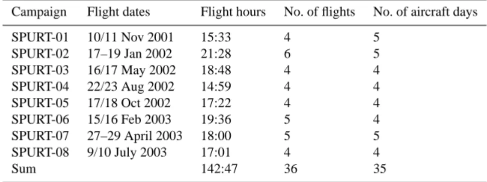
The aircraft used as a platform for the SPURT observa-tions is a Learjet 35A operated by the company GFD (Gesellschaft f¨ur Flugzieldarstellung) in Hohn, Northern Germany (52◦N/6◦E) in cooperation with the company en-viscope. The aircraft reaches a maximum altitude of about 13.7 km and has a range of about 4000 km, while carrying a scientific payload of about 1000 kg. The payload for SPURT consisted of an in-situ gas chromatograph (GhOST II), a tuneable diode laser absorption spectrometer (TRISTAR), a Lyman-α fluorescence hygrometer (FISH), a chemilumines-cence instrument (ECO), an ozone photometer (JOE) and a non-dispersive infrared spectrometer (FABLE). The mea-surement capabilities, including typical precisions and accu-racies, as well as time resolutions are summarised in Table 1. Beside this scientific instrumentation, which is explained in detail in the following sections, standard avionic and me-teorological data were provided by GFD/enviscope. A set of sensors for temperature, differential and static pressure, a data acquisition, and interfaces to the permanently installed aircraft sensors (e.g. GPS antennas, air data computer) was installed in the beginning of each SPURT campaign. This ba-sic instrumentation set allows to retrieve position data, static temperature, static and dynamic pressure, true airspeed and mean horizontal wind speed and direction.
3.1.1 GhOST II
The gas chromatograph GhOST II (Wetter, 2002) is a three channel gas chromatograph, which was developed based on the GhOST instrument described by Bujok et al. (2001). GhOST II compresses outside air by means of a diaphragm pump, then injects samples of this compressed air onto three gas chromatographic columns. Two columns are equipped with ECD detectors for the measurement of CFC 12, SF6
and N2O. These compounds are calibrated relative to the
NOAA/CMDL scale (e.g. Elkins et al., 1993; Montzka et al., 1996). The third column is equipped with a Reduction Gas Detector (RGD) to measure H2and CO. The measurements
are corrected for detector non-linearities and for effects of the cross interference of CO2on the N2O measurements.
3.1.2 TRISTAR
The three channel Tunable Diode Laser Absorption Spec-trometer (TDLAS) TRISTAR (Tracer in situ TDLAS for
Table 1. SPURT measurement equipment. As some of the instruments have been improved during the project, this table reflects the latest
state of the measurement possibilities.
Instrument Institution Technique Species Resolution [s] Precision Accuracy GhOST II JWGU-IMG In-situ GC SF6,
CFC-12, N2O, CO, H2 70 <1% for all, <0.5% for N2O and CFC-12 <2% for all, <1.5% for N2O and CFC-12 TRISTAR MPICH-LC TDL CH4, N2O, CO 5 1% for all species 2% for all species FABLE MPICH-LC IR-spectroscopy CO2 1 0.3 ppm
FISH FZJ-ICG-I Lyman-α H2O 1 <3% 6%
Fluorescence
JOE FZJ-ICG-I O3Photometer O3 10/4 <3% 5% ECO ETH-Z chemiluminescence NO, O3 1 9 pptv,
149 pptv for O3
4.5% for NO, 5% for O3 ETH-Z, AU-converter with NOy 1 11 pptv 16%
MPICH-LC chemiluminescence
atmospheric research, Wienhold et al., 1998; Kormann et al., 2002) was used to measure in situ CO, CH4and N2O. The
ul-timate time resolution of 5 s is determined by the subsequent measurement of each individual channel with an integration time of 1.3 s. The instrument is calibrated in-flight every 10 min against secondary standards of dried compressed air which are cross calibrated against long term laboratory pri-mary standards of NOAA and NIWA. The overall uncertainty is determined from the reproducibility of the in-flight calibra-tions. After post flight data processing we typically achieved a reproducibility of the in-flight calibrations of 1.0%, 1.5% and 2.5%, for N2O, CO, and CH4, respectively. The errors
are slightly larger during ascent and descent. 3.1.3 FABLE
To measure CO2we used the modified Li-COR 6262
NDIR-instrument FABLE (Fast AirBorne Licor Experiment). The instrument was pressure- and temperature-stabilized to min-imize sensitivity changes. Time resolution was 1 Hz and ul-timately limited by the flow rate through the system. The in-strument was in flight calibrated against secondary standards of dried compressed ambient air. To account for the nonlin-earity of the instrument and to guarantee long term stability the setup was cross calibrated against primary standards of NOAA-CMDL with different CO2-content. With this setup
the total uncertainty is estimated to be better than 0.3 ppmv (Gurk, 2003).
3.1.4 FISH
The Fast In-situ Stratospheric Hygrometer (FISH) is an in-strument to measure H2O using the Lyman-α photofragment
fluorescence technique. Details of the instrument are
de-scribed in Z¨oger et al. (1999). The instrument is calibrated in the laboratory before and after each mission and during the SPURT campaigns at each stopover at the home base in Hohn using a calibration bench with a frost point hygrom-eter as a reference instrument. FISH is sensitive to make H2O measurements in the range from about 500–0.2 ppmv in
the UTLS. For stratospheric mixing ratios, the overall accu-racy is 6% and the precision 0.15 ppmv at 1 s time resolution. During SPURT, FISH was equipped with a forward-facing inlet of 10 mm inner diameter. Thus the total water, i.e. the sum of gas-phase and condensed cloud or ice water was mea-sured. Data in clouds are corrected for oversampling in the anisokinetic inlet.
3.1.5 ECO
NOy, NO, and O3were measured using a fast and highly
sen-sitive chemiluminescence analyzer (ECO Physics CLD 790 SR) with three independent channels. Total reactive nitrogen (NOy)was reduced to NO prior to the measurement by using
an externally mounted catalytic gold converter with CO as reduction agent (Fahey et al., 1985; Lange et al., 2002). NO then was measured by chemiluminescence, by letting NO re-act with an excess of O3. O3 was measured based on the
same principle but with an excess of NO. The instrument was calibrated in-flight, before and after each campaign with known amounts of NO, NO2, and O3to account for
chang-ing operatchang-ing conditions such as temperature and pressure that influence the performance of the instrument. The preci-sion of the NOy, NO, and O3data with a resolution of 1 Hz
were 11 pptv, 9 pptv, 149 pptv, respectively. The accuracy of the measurements was 16% for NOy, 4.5% for NO and 5%
A more detailed description of the ECO-instrumentation is given in Hegglin et al. (2005a).
3.1.6 JOE
Ozone was also measured by UV absorption using the J¨ulich Ozone Experiment (JOE). JOE is based on a commercial Thermo Electron Corporation two-stream monitor (model TE 49C) which was modified for operation at reduced pres-sure of the probed air and in the aircraft environment (Mot-taghy, 2001). The instrument was regularly calibrated against a laboratory instrument (TE 49C Primary Standard). The ac-curacy of the ozone monitor is 5% and can be operated to a precision of 2.5 ppbv at an integration time of 10 s. For the use in the SPURT merged data files, JOE data are interpo-lated to 4 or 5 s intervals.
3.2 Instrument intercomparisons
Several trace gases were measured with different instru-ments. In particular O3, N2O and CO were measured by
two instruments which should deliver data of comparable quality. The CO data set obtained from GhOST II is rather small and the instrument was not very well characterized for this species. While in general the tropospheric data of CO showed reasonable agreement between GhOST II and TRIS-TAR, the GC yielded higher values at low mixing ratios. This could either be due to an in-situ CO production in the instru-ment or to a poor detector characterisation. However, the CO data of GhOST II were not used widely, so no thorough data intercomparison has been performed. After the SPURT 7 campaign (see below) an NOyintercomparison flight was
performed with the MOZAIC NOyinstrument (Volz-Thomas
et al., 2005), yielding satisfactory agreement with ECO. Re-sults from this intercomparison is presented in a separate pa-per (Paetz et al., 2006). The intercomparisons detailed in the following, are, therefore, restricted to the N2O and O3data.
3.2.1 Intercomparison JOE-O3and ECO-O3
O3was measured by the Juelich Ozone Experiment (JOE)
using photometry and simultaneously by ECO using chemi-luminescence. Beside the two different measurement tech-niques the two instruments differ by their time resolution of
<1 s for the ECO- and 10 s for the JOE-instrument.
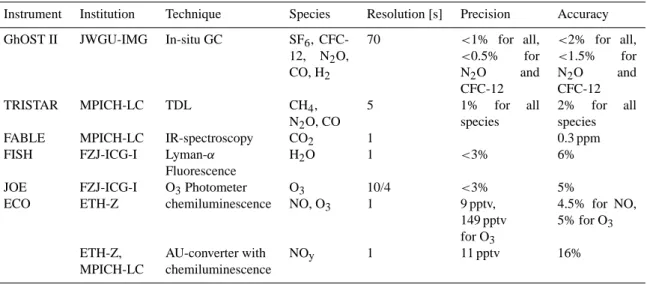
For the following evaluation of the two instruments, the collected data of campaign SPURT 7 (see Sect. 4.2) was chosen due to the large dynamical range between 50 and 1000 ppbv O3. Figure 1 shows the scatter plot of the two
instruments with a linear least-square approximation of the data, taking into account errors in both coordinates. In addi-tion, the expected one-to-one correlation line is given. The correlation was calculated for all data points collected during the five flights of SPURT-7 resulting in a total of 9823 data points. The primary data was merged to 5 s values in averag-ing the ECO O3with a sample rate of 1 s over a 5 s interval
Fig. 1. Least-square approximation of a linear fit between the O3
data from JOE and ECO (red solid line). The dashed blue line indi-cates the one-to-one correlation.
and interpolating the JOE O3with sample rate of 4 s to the
center of each interval. The resulting data is clustered around a straight line with a correlation coefficient of 0.995, indicat-ing that the two data sets are in close agreement. The best linear fit parameters for the slope and the intercept indicate that there is still a significant systematic difference between the two instruments: the slope of 1.064 (±0.002) indicates a 6.4% difference in the two separately collected data sets. This difference is, however, well within the combined over-all uncertainties of the two instruments.
3.2.2 Intercomparison GhOST II N2O and TRISTAR-N2O
As in the case of O3, N2O was measured with two
com-pletely independent techniques on board the Learjet. The TDL spectrometer TRISTAR provides high resolution data at a time resolution of 5 s whereas the GC GhOST II mea-sures N2O with a time resolution of 60 to 90 s (depending
on the chromatographic set-up). Both instruments (or their predecessors) have been intercompared previously (Bujok et al., 2000; Hoor et al., 1999) and were shown to agree within their specified errors. The N2O observations during the
SPURT campaign only span mixing ratios between about 270 and 320 ppbv, giving a low dynamical range, which implies that high precision and accuracy of the data are required. The reproducibility of GHOST II increased due to analytical improvements between SPURT-2 and SPURT-3 from about 1.5% to better than 0.8%. During SPURT-4 and SPURT-5 the precision was better than 0.5%, and about 0.3% during all later measurements. Averaged over all campaigns the mean reproducibility was 0.56%. The precision of the TRISTAR TDL is typically 1% for N2O, being slightly reduced during
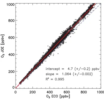
Fig. 2. Direct intercomparision of N2O time series measured by GhOST II (open squares) and by TRISTAR (points). Due to the much
higher sampling frequency, the TDL data set is much larger than the GC data. However, also small scale features are well captured by both instruments, e.g. the spike in the data observed during flight SPURT6 2 around 17:10 UTC.
Fig. 3. Least-square approximation of a linear fit between the N2O
data of TRISTAR and GhOST II. The dynamical range for the cor-relation (red line) is much lower than for ozone (cf. Fig. 1), which results in a lower regression coefficient. The dashed blue line rep-resents the expected 1:1 correlation line.
the initial ascents and final descents and during SPURT-1 and SPURT-2. Figure 2 shows the direct comparison between TRISTAR and GhOST II observations during the flights of
the SPURT-6 campaign. Even small scale structures are re-produced very well by both instruments. Figure 3 shows the scatter plot between GHOST II observations and TRISTAR measurements at the same time (due to the higher time res-olution of TRISTAR only a small fraction of the TRISTAR data are included in the plot). The scatter around the regres-sion line is 0.91% (1 sigma), which is well below the com-bined stated precisions of both instruments, showing that the error estimates are conservative.
3.3 Data post-processing
Measurements from the different instruments were obtained at different sampling intervals and at different time lags due to the varying sampling properties and instrumental response times. A cross-correlation analysis was therefore performed on pairs of observations from a single flight in order to assess a time lag correction for each instrument. These corrections were in the range of 1 to 8 s depending on the instrument and were found to vary by no more than 1 to 2 s between the different flights and campaigns.
Data recorded by the individual instruments and the Lear-jet flight data system were finally combined into a single “merge file” with a time resolution of 5 s, which is avail-able for each flight in addition to the instrument-specific data files. Meteorological data from operational ECMWF anal-ysis fields interpolated from the model grid onto the flight tracks were also included in the merge files. ECMWF data with a three hour time resolution, 60 vertical layers and
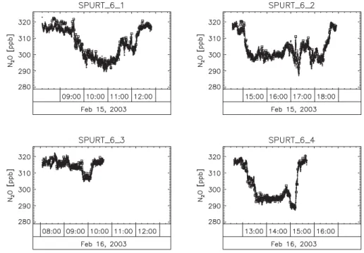
Table 2. SPURT campaigns, with dates, number of flight hours, number of flights and number of days the aircraft was booked.
Campaign Flight dates Flight hours No. of flights No. of aircraft days SPURT-01 10/11 Nov 2001 15:33 4 5 SPURT-02 17–19 Jan 2002 21:28 6 5 SPURT-03 16/17 May 2002 18:48 4 4 SPURT-04 22/23 Aug 2002 14:59 4 4 SPURT-05 17/18 Oct 2002 17:22 4 4 SPURT-06 15/16 Feb 2003 19:36 5 4 SPURT-07 27–29 April 2003 18:00 5 5 SPURT-08 9/10 July 2003 17:01 4 4 Sum 142:47 36 35
a 1.0×1.0 degree resolution were used. These files com-prise temperature, winds, humidity, potential vorticity, and equivalent latitude. Equivalent latitude (φe)versus PV
rela-tions were first calculated from the PV distriburela-tions on 14 isentropic surfaces between 270 and 400 K to obtain a two-dimensional field φe (PV, θ ), which was then linearly
inter-polated onto the ECMWF model PV and potential tempera-ture values along the flight track.
10-day backward trajectories based on 3-hourly ECMWF fields of horizontal and vertical winds were started every 10 s along the flight track using the LAGRANTO trajectory tool (Wernli and Davies, 1997). Minimum and maximum val-ues of PV, temperature, latitude and relative humidity along the trajectories as well as the number of hours since the last tropopause crossing (defined as change from above/below to below/above 2 PVU) were also stored in the merge files. All these ancillary data proved useful for the analysis and inter-pretation of the observations.
3.4 Data availability
The data can be freely downloaded from http://www.iac.ethz. ch/spurt/ provided a simple user data protocol is agreed on, stating that the instrument PIs should be informed about the use of their data at an early stage of the investigation and that co-authorship should be offered for publications making use of these data.
4 The measurement strategy and the SPURT cam-paigns
4.1 The measurement strategy
As the aim of SPURT was to provide observations under typ-ical conditions of the UT/LMS region during all seasons, we performed a total of eight measurement campaigns within an observational period of 2 years from November 2001 until July 2003, probing each season twice. The flight routes of each campaign were covering the UT/LMS in the European
longitude sector from high Northern latitudes to the subtrop-ics as far equatorward as possible. In order to achieve this goal under reasonable costs, the campaigns had to be organ-ised in a very efficient way. All instruments were designed to allow fast mounting on the aircraft and were able to mea-sure within one single day. Because of capacity constrictions, only 2 operators were allowed to participate in the flights and thus the instruments had to be automated, so that they could be operated with minimal interference from the board crew. This strategy proved to be very successful, since we were able to perform a SPURT campaign within five days. A typi-cal campaign started with two and a half days for integration and instrument checks on board (including an aircraft seal property test and mass distribution assessment), followed by a first flight day going northward or southward and the sec-ond flight day heading in the opposite direction on the fol-lowing day, provided that no instrument failures occurred. Table 2 shows a summary of the dates, the amount of flight hours and the amount of aircraft booking days for each cam-paign. The SPURT strategy allowed us to keep aircraft dry leasing costs low, by flying under the given meteorological conditions on fixed days and spending only a minimum time for integrating and testing the instruments.
The two flight days were fixed from the beginning of the campaign and it was our strategy not to wait for any specific meteorological situation with the advantage, that the SPURT data set is not biased by specific conditions. To optimise the flight route, we used the meteorological forecasts prepared by the ETH Z¨urich based upon operational forecast data from ECMWF for flight planning. The flight in each direction then consisted of an outbound flight, a refuelling stop after about 4 flight hours and then a second flight back to the aircraft base at Hohn. Optionally, the second flight would go further outbound and the base at Hohn would only be reached af-ter a second refuelling stop. In order to achieve an optimal sampling of the UT/LMS the first part of a flight usually con-sisted of a first level just above the tropopause in the vicinity of the strongest PV-gradients and a second level well above the tropopause. This pattern was mirrored on the return flight
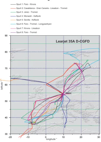
- 2 0 - 1 0 0 1 0 2 0 3 0 3 0 4 0 5 0 6 0 7 0 8 0 9 0 S p u r t 6 : F a r o - T r o m s ö - L o n g y e a r b y e n H o h n e n v i s c o p e G m b H la tit ud e ° l o n g i t u d e ° L e a r j e t 3 5 A D - C G F D S P U R T 1 t o 8 f l i g h t t r a c k s S p u r t 5 : S e v i l l a - K e f l a v i k S p u r t 4 : M o n a s t i r - K e f l a v i k S p u r t 3 : J e r e z - T r o m s ö S p u r t 2 : C a s a b l a n c a - G r a n C a n a r i a - L i s s a b o n - T r o m s ö S p u r t 1 : F a r o - K i r u n a - 2 0 - 1 0 0 1 0 2 0 3 0 3 0 4 0 5 0 6 0 7 0 8 0 9 0 S p u r t 7 : K i r u n a - L i s s a b o n S p u r t 8 : F a r o - T r o m s ö
Fig. 4. Flight path of the Learjet for all 8 SPURT measurement
campaigns.
on the same day such that each geographical location was sampled twice at two different altitudes. Before each land-ing the aircraft climbed to maximum altitude followed by a slow descent to the airport in order to obtain highly resolved vertical profiles. Since the airports chosen for intermediate stops mostly were rather small remote airports, we were able to measure clean air vertical profiles during the descent into the airports. The flight path of the Learjet for all campaigns is shown in Fig. 4.
4.2 The campaigns
In the following section we give a brief overview of the in-dividual SPURT campaigns, including the dates, flight direc-tions, the meteorological setting, and general information on instrument performance or failures. No details on the indi-vidual flights are given, since this would be beyond the scope of this paper. The SPURT campaigns are named chronologi-cally, starting with SPURT-1. If reference is made to an indi-vidual flight, the campaign number is followed by the flight number. E.g. flight S3.2 denotes the second flight of the third SPURT campaign. The data availability for the individual flights is summarised in Table 3. Table 4 summarises some
meteorological parameters, the locations, the maximum O3
and the minimum N2O mixing ratios for all the individual
flights, as an indication on how deep the individual flights reached into the LMS:
4.2.1 SPURT-1: 10/11 November 2001
During the first autumn campaign the aircraft flew south to Faro (Portugal), reaching 35◦N on 10 November 2001.
The aircraft was crossing a deep upper level trough dur-ing the southbound flight and was flydur-ing mostly within the troposphere on the return flight conducted to the west of the trough. The meteorological situation and the measure-ments during the first flight were described in detail in the case study of Hegglin et al. (2004). On 11 November the northbound leg with a refuelling stop over Kiruna (Sweden) reached 73◦N before returning to Hohn. All instruments ex-cept GHOST II worked well during this campaign. CO2data
are not available for flight S1.2. 4.2.2 SPURT-2: 17–19 January 2002
During the first winter campaign the aircraft first headed south to Casablanca, flying mostly within a narrow strato-spheric streamer stretching from Great Britain to northern Africa, and then proceeded further south. Due to an over-heated fan in the aircraft ventilation system an emergency landing on the Canary Island was necessary. The aircraft reached 27◦N during this campaign, where the southern-most data available from SPURT were taken. After repair the aircraft returned to Hohn and continued northwards on 19 January, with a refuelling stop in Troms¨o (Norway). A tro-pospheric streamer associated with an elevated tropopause extending from central Europe to Scandinavia was probed twice on these flights to and from Troms¨o. Again, the north-ernmost data from this campaign are from about 73◦N. Data are available from all instruments for this campaign, although some GC data (Flight S2.4) are lacking.
4.2.3 SPURT-3: 16/17 May 2002
The synoptic situation during this campaign was dominated by high pressure conditions over central Europe. Again the aircraft first headed south, refuelling in Jerez (Spain). Most of this flight took place in the vicinity of the tropopause. The southern edge of the data available from this campaign is at 36◦N. The northbound flights on 17 May reached deep into the stratosphere over Scandinavia and extended as far north as 75◦N. The stopover was in Troms¨o (Norway). Data are available from all instruments for this campaign, the GC data are only complete for SF6.
4.2.4 SPURT-4: 22/23 August 2002
Entire Europe was characterized by a flat pressure distribu-tion and a relatively high tropopause. A moderate cyclone
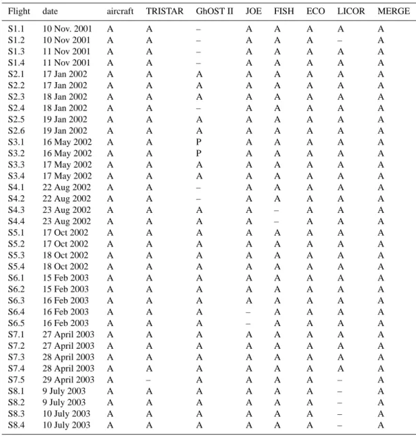
Table 3. SPURT data availability, sorted by instrument for each flight. A = data available, P = data partly available, – = no data. As O3and
N2O were measured by two instruments, data for these species are available for all flight. Water vapour is missing for 2 flights, CO2for 5
flights and SF6for 7 flights. NOydata ar available for all flights.
Flight date aircraft TRISTAR GhOST II JOE FISH ECO LICOR MERGE S1.1 10 Nov. 2001 A A – A A A A A S1.2 10 Nov 2001 A A – A A A – A S1.3 11 Nov 2001 A A – A A A A A S1.4 11 Nov 2001 A A – A A A A A S2.1 17 Jan 2002 A A A A A A A A S2.2 17 Jan 2002 A A A A A A A A S2.3 18 Jan 2002 A A A A A A A A S2.4 18 Jan 2002 A A – A A A A A S2.5 19 Jan 2002 A A A A A A A A S2.6 19 Jan 2002 A A A A A A A A S3.1 16 May 2002 A A P A A A A A S3.2 16 May 2002 A A P A A A A A S3.3 17 May 2002 A A A A A A A A S3.4 17 May 2002 A A A A A A A A S4.1 22 Aug 2002 A A – A A A A A S4.2 22 Aug 2002 A A – A A A A A S4.3 23 Aug 2002 A A A A – A A A S4.4 23 Aug 2002 A A A A – A A A S5.1 17 Oct 2002 A A A A A A A A S5.2 17 Oct 2002 A A A A A A A A S5.3 18 Oct 2002 A A A A A A A A S5.4 18 Oct 2002 A A A A A A A A S6.1 15 Feb 2003 A A A A A A A A S6.2 15 Feb 2003 A A A A A A A A S6.3 16 Feb 2003 A A A A A A A A S6.4 16 Feb 2003 A A A – A A A A S6.5 16 Feb 2003 A A A – A A A A S7.1 27 April 2003 A A A A A A A A S7.2 27 April 2003 A A A A A A A A S7.3 28 April 2003 A A A A A A A A S7.4 28 April 2003 A A A A A A A A S7.5 29 April 2003 A – A A A A – A S8.1 9 July 2003 A A A A A A – A S8.2 9 July 2003 A A A A A A – A S8.3 10 July 2003 A A A A A A – A S8.4 10 July 2003 A A A A A A – A
was located near Iceland. In order to cross the tropopause on a high flight level we flew south to Monastir (Tunisia), reaching 33◦N on 22 August where we expected to measure subtropical tropospheric air at high altitudes. On 23 August the northbound measurements were carried out. This is one of the two occasions when we chose to fly northwest instead of north, in order to reach deep into the stratosphere over Ice-land where a low tropopause was predicted. The refuelling stop was in Keflavik (Iceland), and data are available up to a latitude of 64◦N. No GC data are available for the south-bound flights and on the northsouth-bound flights water vapour data are missing. All other instruments worked nominally.
4.2.5 SPURT-5: 17/18 October 2002
The second autumn campaign took place after the passage of a low pressure system over northern Germany mostly in a region with a low tropopause. Again we flew southward on the first measurement day, refuelling in Sevilla (Spain) and reaching the southernmost latitude of 35◦N on the flight back. The northbound leg went to Keflavik towards an iso-lated tropospheric air mass, and the northernmost datapoints are from 64◦N. This campaign has the most complete data set of all, as all instruments worked nominally during all flights.
Table 4. SPURT flight coverage: Length of flight, maximum western longitude (◦W are negative), maximum eastern longitude, minimum and maximum latitude reached by the Learjet. The maximum 2 and 12 levels, as well as the minimum N2O levels and the maximum O3
levels observed during the flights are also shown.
Flight date Flight Hours Lon west Lon east Lat min Lat max 2max 12max PV max O3max N2O min
hh:mm [◦] [◦] [◦] [◦] [K] [K] [PVU] [ppbv] [ppb] S1.1 10 Nov 2001 04:10 –9.83 9.56 35.78 54.32 370.1 66.3 10.4 659.3 293.4 S1.2 10 Nov 2001 04:11 –8.42 9.52 37.01 54.29 362.1 2.0 2.7 115.0 309.8 S1.3 11 Nov 2001 02:44 9.37 21.39 54.29 68.66 370.0 71.7 8.7 538.5 296.8 S1.4 11 Nov 2001 04:01 9.68 25.24 54.19 73.12 367.6 69.6 9.0 580.6 294.7 S2.1 17 Jan 2002 04:24 –8.22 9.56 33.49 54.34 365.4 52.0 8.6 397.4 300.2 S2.2 17 Jan 2002 01:21 –14.44 –7.77 27.50 33.33 342.0 18.7 6.1 212.5 311.0 S2.3 18 Jan 2002 02:27 –15.39 –7.69 27.92 38.60 363.1 25.7 8.1 280.2 303.0 S2.4 18 Jan 2002 03:25 –9.14 9.56 38.77 54.14 360.9 28.2 9.0 398.1 302.6 S2.5 19 Jan 2002 04:27 0.11 19.20 54.31 73.20 361.7 58.3 8.6 693.9 285.7 S2.6 19 Jan 2002 04:16 0.10 19.07 54.39 73.13 372.2 65.8 9.0 693.3 286.3 S3.1 16 May 2002 04:40 –8.68 9.63 36.13 54.32 355.5 16.3 7.4 376.9 296.5 S3.2 16 May 2002 04:21 –13.92 8.85 36.72 54.22 369.4 40.1 9.9 670.7 281.0 S3.3 17 May 2002 04:24 9.25 24.00 54.28 75.10 372.6 67.5 8.5 790.9 279.7 S3.4 17 May 2002 04:34 5.02 18.97 47.85 69.75 371.6 31.9 8.4 686.5 280.8 S4.1 22 Aug 2002 03:47 9.52 13.60 33.80 54.32 363.1 22.8 9.3 364.6 300.6 S4.2 22 Aug 2002 03:26 8.33 11.86 35.72 54.52 370.9 40.2 9.4 448.7 298.6 S4.3 23 Aug 2002 03:36 –27.21 9.76 54.31 65.05 370.4 56.9 10.2 435.2 301.6 S4.4 23 Aug 2002 03:44 –22.63 9.75 53.34 63.99 364.6 36.5 9.2 371.9 303.6 S5.1 17 Oct 2002 04:26 –7.03 9.56 36.50 54.32 359.0 43.8 8.2 266.7 306.3 S5.2 17 Oct 2002 04:25 –8.00 9.89 35.42 54.27 373.2 64.0 9.3 356.4 306.7 S5.3 18 Oct 2002 04:11 –26.27 9.56 53.71 63.71 365.4 42.8 9.3 300.3 309.4 S5.4 18 Oct 2002 03:35 –26.63 9.40 54.27 64.11 371.1 65.4 8.9 509.3 303.4 S6.1 15 Feb 2003 04:30 –12.00 9.68 36.84 54.32 362.6 60.7 8.0 711.1 291.9 S6.2 15 Feb 2003 04:21 –7.97 10.02 37.00 54.25 373.2 69.9 9.1 708.3 291.9 S6.3 16 Feb 2003 02:50 9.55 18.54 54.31 69.85 354.5 37.0 7.5 364.6 307.4 S6.4 16 Feb 2003 03:32 10.02 30.08 69.54 82.07 356.8 57.9 8.9 751.7 288.9 S6.5 16 Feb 2003 03:35 9.34 19.08 54.36 78.26 358.5 40.3 9.1 503.6 300.2 S7.1 27 April 2003 04:10 9.37 21.00 54.29 72.99 378.2 77.1 9.0 1049.9 263.2 S7.2 27 April 2003 04:38 8.43 20.35 49.99 70.53 373.6 60.7 8.2 736.4 285.2 S7.3 28 April 2003 04:29 –10.39 9.54 38.50 54.31 355.6 27.9 7.1 645.1 289.1 S7.4 28 April 2003 04:16 –10.19 13.44 37.95 54.51 366.7 43.3 9.3 657.9 288.4 S7.5 29 April 2003 04:12 9.42 15.60 53.27 66.09 367.1 47.9 8.3 746.1 284.9 S8.1 9 July 2003 03:56 –8.70 9.56 35.88 54.32 363.8 34.0 9.3 430.4 300.1 S8.2 9 July 2003 04:20 –8.05 9.55 35.87 54.47 365.3 32.4 8.0 469.4 299.3 S8.3 10 July 2003 03:57 9.30 21.82 54.29 73.25 372.2 66.2 10.9 559.0 292.8 S8.4 10 July 2003 04:05 6.54 21.75 49.90 69.69 367.2 34.7 10.1 567.6 291.1 4.2.6 SPURT-6: 15/16 February 2003
During this campaign a very prominent high-pressure sys-tem was situated over middle and northern Europe and there-fore the tropopause was generally quite high. The south-bound flight to Faro (Portugal) took place on 15 February and reached 36◦N. The northbound leg on 16 February went to Longyearbyen (Spitsbergen) after a stop over in Troms¨o (Norway). Data are available from as far north as 82◦N and are the most poleward data available from SPURT. Only ECO (chemiluminescence) provided ozone data during the flight S6.4 and 6.5. All other data are complete.
4.2.7 SPURT-7: 27–29 April 2003
Europe was divided meteorologically into two broad regions during this campaign, a low pressure area towards the north-west (with a centre between Scotland and Iceland) and a high pressure area over the southern and eastern parts. The northbound flight took place on 27 April and reached 73◦N. The stopover airport was Kiruna (Sweden). The southbound flights took place on 28 April, with a stopover at Lisbon (Por-tugal) and southernmost datapoints around 38◦N . After this campaign, an extra flight for intercomparison of NOy
the NOyinstrument used for the MOZAIC programme
(Volz-Thomas et al., 2005) was added to the payload, the TDL and the CO2instrument had to be removed for this extra flight.
4.2.8 SPURT-8: 9–10 July 2003
The final campaign took place in a region between a mature Icelandic Low and an anticyclone over Russia. Over south-western Europe the ECMWF data show a richly structured tropopause with slowly evolving filaments of tropospheric and stratospheric air. The southern flights were performed on 9 July and the stopover airport was again Faro (Portugal) and data are available down to 36◦N. The northbound flights on 10 July reached 73◦N with refuelling at Troms¨o (Norway). Data from this campaign are complete, with the exception of CO2, which is not available.
5 Data overview
In the frame of the SPURT project a large number of data has been collected in the UT/LMS for a wide range of trac-ers. For many tracers (e.g. N2O, SF6, CO2) the observed
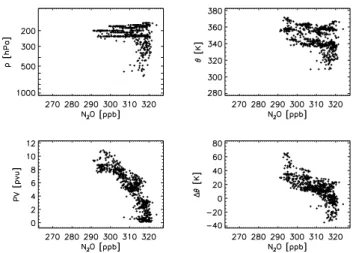
variabilities are very small. It should also be noted that the LMS is a dynamically very active region. Representing the data in classical co-ordinate systems does not show the fea-tures of the typical distributions. This is illustrated in Fig. 5, where the distribution of N2O measured during campaign S8
is plotted vs. pressure, potential temperature, potential vor-ticity and Theta above the local tropopause (note that the local tropopause is calculated form the ECMWF data). It is clearly visible that the complete range of N2O values
ob-served is present at all pressures below about 250 hPa and all potential temperatures above about 340 K. A systematic structure is only clear when using PV or Theta above the local tropopause as vertical coordinates, i.e. vertical scales which hold some tropopause information. Therefore, in or-der to give an overview of the data collected during SPURT, the measurements of N2O, CO, O3, SF6, CO2, H2O and NOy
will be presented in the equivalent latitude – potential tem-perature coordinate system, and grouped by season. Since the distributions of CFC-12 and CH4are very similar to those
derived from N2O, they will not be presented separately. For
all distributions shown below, the data from the two cam-paigns in each season have been combined and binned on a 5◦equivalent latitude/5 K potential temperature grid. A mean
from all measurements inside each grid box was then calcu-lated. In the case of N2O two instruments (TRISTAR and
GhOST II) provided data, with different temporal resolutions and precisions, the GC GhOST II having a higher precision than the TDL TRISTAR. The mean values given for each box represents an average of TDL and GC data, each measure-ment point being weighted according to its precision (e.g. a single GHOST II observation with 0.5% precision would be weighted twice as heavily as a TRISTAR measurement point
Fig. 5. Distribution of N2O derived from GhOST II measurements
during campaign S8, as a function of different vertical scales. Only vertical scales including tropopause information (i.e. PV or 12) can reveal the systematic structure of the distribution, wheras scales like pressure (p) or 2 show a large scatter in the data
with 1% precision). In the case of O3the data from the UV
photometer JOE were used as these are available over the entire time frame of the project, with the exception of two flights during February 2003. For these flights the chemi-luminescence measurements by the ECO instrument were used.
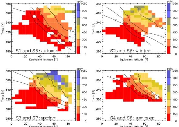
5.1 Nitrous oxide – N2O
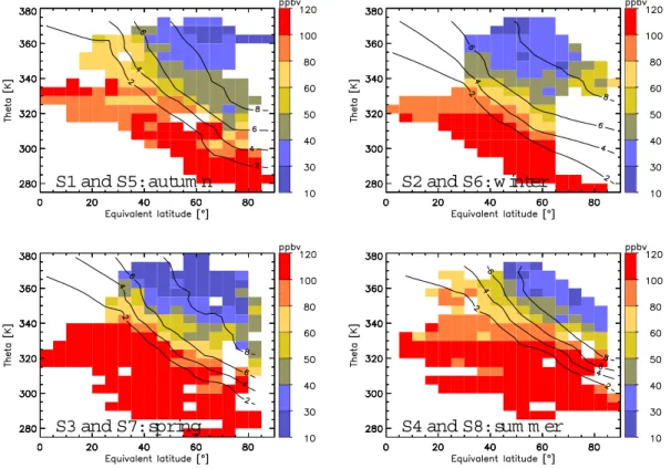
Nitrous oxide shows very uniform values in the troposphere (Fig. 6). For example during the campaigns in 2003 the GhOST II measured mean tropospheric N2O values between
318.3±1.5 (1 sigma standard deviation) in February 2003 and 318.8±1.4 ppb in July 2003. The standard deviations include the instrumental precisions, which is on the order of 1 ppb. These data agree very well with the values from the NOAA/CMDL network (e.g. Elkins et al., 1993, up-dated), which show N2O mixing ratios of 318.2±0.4 ppb
and 318.4±0.7 ppb for the respective time periods. With the exception of the spring season, values very close to the tropospheric mean are observed up to PV values of 4 to 6 PVU depending on season. The lowest N2O values
are observed during spring. The minimum N2O value
ob-served during SPURT was 263 ppb during flight S7.1. during other spring time flights the lowest values were on the order of 280 ppb. The highest, i.e. most tropospheric values are found during autumn. During the autumn campaign SPURT-1 in November 200SPURT-1, the lowest N2O observations were
around 294 ppb, and during the second autumn campaign (SPURT-5 in October 2002) no N2O values below 300 ppb
were observed. Note the similarity between the distributions observed during winter and summer and the tilt of the iso-pleths relative to isentropes.
S1 and S5: autum n S2
and S6: w inter
S3 and S7: spring S4
and S8: sum m er
Fig. 6. Observed distribution of N2O sorted by season as function of equivalent latitude and potential temperature. Data are from the TDL TRISTAR and the GC GhOST II. The black lines represent different PV isopleths (2, 4, 6 and 8 PVU). The 2 PVU isopleth is often used as the dynamical tropopause.
S1 and S5: autum n S2
and S6: w inter
S3 and S7: spring S4
and S8: sum m er
5.2 Carbon monoxide – CO
The distribution of CO derived from SPURT (Fig. 7) has been discussed previously by Hoor et al. (2004a, b). CO shows higher variability than N2O in the troposphere and
a latitudinal gradient, with lower mean values in the up-per troposphere at low latitudes. CO has a much shorter lifetime than e.g. N2O, on the order of 3 months, but also
has a stratospheric source from methane oxidation. In the background stratosphere typical values below 15 ppb are ex-pected. Such low mixing ratios are only observed far away from the tropopause in the overworld at altitudes exceeding the SPURT flight ceiling. Average values below 40 ppb are only observed for PV>6 PVU, which is only the case at a dis-tance of at least 1θ =20 to 30 K above the local tropopause. 5.3 Ozone – O3
Ozone has its main sources in the stratosphere. Ozone is not an inert tracer in the lowermost stratosphere, like e.g. N2O.
Yet the chemical lifetime of the odd oxygen (Ox)- family is
well above 1 year in the lower stratosphere below 20 km (see e.g. Brasseur and Solomon, 1986). Therefore the distribu-tion of ozone in the lowermost stratosphere is dominated by transport rather then chemistry.The seasonal changes of up-per tropospheric ozone are not resolved in the figures shown below. Note, however, that the SPURT data show O3values
in the tropopause region (2–3 PVU) in spring and summer being about 60% higher than corresponding values in autumn and winter (see also Hegglin et al., 2005a; Krebsbach et al., 2005a). This seasonal variation is generally smaller at 5– 6 km, which is considered to be representative of the free tro-posphere, since it is rather weakly influenced by small scale anomalies of the tropopause height and by local emissions of O3precursors that generally take place in the boundary layer
(Fischer et al., 2005). As in the case of N2O the most
strato-spheric values are observed in the upper part of the LMS dur-ing sprdur-ing, where maximum values close to 1000 ppbv were observed (Fig. 8). Much lower values were measured during the other seasons. The ozone isopleths very closely follow the PV isolines. During summer and even more pronounced during autumn, a region of rather low ozone is observed in the lowermost stratosphere up to PV values of 4 to 6 PVU between about 20 and 40 degrees of equivalent latitude. 5.4 Sulfur hexafluoride – SF6
Sulfurhexafluoride is an extremely long lived atmospheric trace gas, which has its only sink in the mesosphere. In con-trast to most of the other tracers measured during SPURT, the vertical gradient observed in SF6is not caused by chemistry
but is rather due to the time lag with which the tropospheric increase propagates into the LMS. It is therefore not possible to combine SF6data from different years without
account-ing for the long-term trend. Therefore, we present the SF6
data from the second annual cycle, based on the SPURT cam-paigns 5 to 8 (Fig. 9), which provide a complete SF6data set.
Again, the air with the strongest stratospheric influence is ob-served during spring, where the lowest mixing ratios of SF6
were found. As with many other tracers, the distribution of SF6closely follows the PV isolines. Note that SF6increases
in the troposphere at a rate of about 4 to 5% per year (i.e. about 0.1 ppt per year). This is reflected by the higher values of SF6in the summer (the SPURT-8 campaign took place in
July 2003) than in autumn (SPURT-5 was carried out in Oc-tober 2002).
5.5 Carbon dioxide – CO2
Similar to SF6, CO2also has a sufficiently long atmospheric
lifetime to reveal its long-term trend in the stratosphere. In addition, CO2 has a pronounced seasonal cycle in the
tro-posphere, due to the uptake and release by vegetation. The distribution of CO2 (Fig. 10) therefore shows a unique
pat-tern. As is the case of SF6, only one seasonal cycle is shown,
as the long term increase could otherwise mask the seasonal variability. Since the data set for the first seasonal cycle is more complete, we present the results from SPURT-1 to 4. During SPURT-1 in Autumn 2001 very little variability of CO2was observed throughout the LMS. During winter and
spring, the CO2values in the LMS are mostly below the
tro-pospheric values. On the contrary, during summer, CO2was
higher in the stratosphere than in the troposphere. This par-ticular behavior of CO2was described by Hoor et al. (2004b),
who suggested that a large part of the air in the lowermost stratosphere with elevated CO2(as well as CO>15 ppb) was
caused by relatively fast transport from the upper tropical tro-posphere, where tropospheric summertime CO2 values are
higher than in the mid latitude during the same period. 5.6 Reactive nitrogen – NOy
Reactive nitrogen (NOy)is the sum of all reactive nitrogen
species with an oxidation state higher than one. The produc-tion of reactive nitrogen is initiated in the stratosphere due to reaction of N2O with O(1D). In addition, sources due to
lightning, deep convective injection of planetary boundary layer air, and air traffic emissions may influence the budget of NOyin the UT/LMS. Figure 11 shows the observed
distri-butions of NOy. As the scale is reversed (i.e. the blue colours
show the highest values) with respect to Fig. 5 (N2O
distribu-tion), the distributions look very similar. The highest values of NOyare observed during spring in the highest part of the
LMS, again indicating the strongest stratospheric influence during this time of the year. Conversely, the summer and autumn distributions reveal significant influence of transport from the troposphere. A detailed discussion of the observed NOy tracer distributions and implications for the origin of
air masses in the lowermost stratosphere as obtained from tracer-tracer correlations is given by Hegglin et al. (2005a).
S1 and S5: autum n S2
and S6: w inter
S3 and S7: spring S4
and S8: sum m er
Fig. 8. As Fig. 6, but for O3. Data are from the UV photometer JOE and partly from the chemiluminescence instrument ECO.
S5: autum n S6: w inter
S7: spring S8: sum m er
S1: autum n S2: w inter
S3: spring S4: sum m er
Fig. 10. As Fig. 6, but for CO2. Only one seasonal cycle is included. Data are from the non-dispersive IR CO2analyzer FABLE.
S1 and S5: autum n S2
and S6: w inter
S3 and S7: spring S4
and S8: sum m er
S1 and S5: autum n S2
and S6: w inter
S3 and S7: spring S4
and S8: sum m er
Fig. 12. As Fig. 6, but for H2O. Data are obtained using the Lyman-α hygrometer FISH.
5.7 Total water – H2O
Water is a tracer which is strongly influenced by freeze-drying during the transport into the LMS. The highest mix-ing ratios of H2O are observed during summer and the lowest
values during autumn (Fig. 12). This seasonality is in accor-dance with other observations of H2O in the LMS
(Krebs-bach et al., 2005b1and references therein) but differs clearly from other tracers observed during SPURT, which show the most pronounced tropospheric influence a few months later. The difference must be explained by the different mecha-nisms controlling water vapour in the LMS and its large gradients at the tropopause which make H2O a very
sen-sitive indicator for cross-tropopause transport. During the transit from summer to autumn very dry air appears to be transported into the lowermost stratosphere. Water vapour is also the tracer which shows most significantly the tro-pospheric influence even at rather large distances from the local tropopause. One reason is again that H2O
concentra-tions have by far the largest contrast between tropospheric and stratospheric values. Further, there are practically no sinks of water vapour in the LMS except freeze-drying at the coldest point which is located near the tropopause. Thus, once humid air masses have entered the LMS, they can only be diluted with drier stratospheric background air and be re-moved from the LMS by transport. Finally, the efficiency of freeze-drying at the tropopause shows a strong seasonal cycle and latitudinal dependence, overlaid by episodic short-term
variability. Detailed investigations of H2O transport across
the extratropical tropopause and its seasonality are given in specific studies (Krebsbach et al., 2005a, b1).
6 Conclusions and outlook
SPURT has provided a comprehensive data set of trace gases for the lowermost stratosphere (LMS) in the Northern Hemi-sphere. This data set is of high quality and contains a number of important trace gases with different lifetimes and differ-ent source/sink characteristics. Species with differdiffer-ent life-times can give information on different chemical and trans-port processes (see e.g. Tuck et al., 2004). The SPURT data set also provides an ideal basis for studies of meso- and small-scale troposphere-to-stratosphere transport processes (e.g. isentropic or associated with deep convection) and their impact on lowermost stratospheric trace gas distributions. The high quality of the data set is evident from the inter-comparison between the simultaneously measured N2O (by
GC and TDL) and O3 (by UV absorption and
chemilumi-nescence). Both intercomparisons show an agreement which is better than the stated combined uncertainties of the in-struments over the entire range of values. In several stud-ies we show, that by using an adequate coordinate system (potential temperature and equivalent latitude) much of the natural variability, which is due to reversible synoptic-scale processes, can be removed from the data (e.g. Hoor et al., 2004a, b; Hegglin et al., 2005a; Krebsbach et al., 2005a, b1).
Presenting the data in this coordinate system, clear season-alities in the lowermost stratosphere are observed. Over the course of the winter and into spring, the LMS is filled up with air of marked stratospheric character, which has com-paratively low mixing ratios of N2O, SF6, CO, and H2O but
relatively high mixing ratios of ozone and NOy. This air is
replaced over the summer and into autumn by air of more tropospheric character, having higher mixing ratios of N2O
and SF6and lower mixing ratios of NOyand ozone. Within
the SPURT project the driest air in the lowermost strato-sphere was observed during autumn and winter, whereas the moistest air was present in summer. The SPURT observa-tions reveal a tropopause following transition layer (Hoor et al., 2004b, 2005; Hegglin et al., 2005b; Krebsbach et al., 2005b1), showing trace gas mixing ratios intermediate be-tween typical tropospheric and stratospheric values. This layer shows seasonal variability and slightly varying thick-ness, depending on the trace gases used for its determination and the elapsed time since the mixing occurs (e.g. Hoor et al., 2004a, 2005; Krebsbach et al., 2005b1). The SPURT data confirm that the LMS is a mixture of air from the overworld and from the extratropical upper troposphere (e.g. Hoor et al., 2004b; Hegglin et al., 2005b), as is also assumed in some budget studies (e.g. Ray et al., 1999). However, another im-portant pathway influencing the lowermost stratosphere is fast transport of upper tropospheric air from the tropics, as evidenced in the seasonal cycle of CO2or of tracer-tracer
cor-relations (e.g. Hoor et al., 2004b, 2005; B¨onisch et al., 20052; Hegglin et al., 2005a). Isentropic transport (e.g. through ex-change near the sub-tropical tropopause break) or transport via the tropically controlled transition layer (Rosenlof et al., 1997) in the extratropical lower stratosphere could explain these observations. Budget studies allow investigating the seasonality of the influence of different source regions on the LMS (e.g. B¨onisch et al., 20052), indicating that depending on season 30–50% of the air in the LMS originate at the trop-ical tropopause (Hoor et al., 2005).
Accompanying modelling work focuses on transport of air into the lowermost stratosphere, using the SPURT observa-tions to compare the model results with atmospheric reality. The SPURT data set is ideally suited for the initialisation and systematic evaluations of models, in particular for transport studies and budget investigations in the UT/LMS on regional up to hemispherical scales, and for investigations of seasonal variability. Several studies using a simple 2-D model (Heg-glin et al., 2005a) up to full 3-D Lagrangian CTM (CLaMS) have been carried out or are under preparation (G¨unther et al., 20053; Pan et al., 2006). SPURT data have also been applied
2B¨onisch, H., Engel, A., Schmidt, U., et al.: A budget study
of air mass origin in the lowermost stratosphere based on in-situ observations of CO2and SF6during SPURT, in preparation, 2005.
3G¨unther, G., Konopka, P., Krebsbach, M., and Schiller, C.: The
quantification of water vapor transport in the tropopause region us-ing a lagrangian model, in preparation, 2005.
to assimilation techniques (Elbern and Strunk, 2005). Case studies of atmospheric transport in the UT/LMS for specific SPURT missions are carried-out using e.g. Reverse Domain Filling (RDF) techniques or a parameterised convective influ-ence analyses (e.g. Hegglin et al., 2004; Krebsbach, 2005). Detailed investigation of backward trajectories together with the trace gas observations reveal important aspects for in-stance of TST events. Finally, the SPURT campaign spurred more theoretical work on fundamental properties of tracer advection in the extratropical tropopause region (Wirth et al., 2005) and on the sharpness of the extratropical tropopause during baroclinic development (Szabo and Wirth, 20064).
Acknowledgements. We would like to thank the Gesellschaft f¨ur
Flugzieldarstellung (GFD) for the excellent co-operation and sup-port during the aircraft campaigns. Funding of the project under the AFO 2000 programme of the German Ministry for Education and Research (BMBF) is gratefully acknowledged.
The Institute for Atmospheric and Climate Science (ETH) thanks the Swiss National Fund for its support of the NOy-, NO-, and
O3-instrumentation and MeteoSwiss for granting access to the
ECMWF data. Edited by: P. Haynes
References
Appenzeller, C., Holton, J. R., and Rosenlof, K. H.: Seasonal vari-ation of mass transport across the tropopause, J. Geophys. Res., 101(D10), 15 071–15 078, doi:10.1029/96JD00821, 1996. Boering, K. A., Daube, B. C., Wofsy, S. C., Loewenstein, M.,
Podolske, J. R., and Keim, E. R.: Tracer-tracer relationships and lower stratospheric dynamics: CO2and N2O correlations during
SPADE, Geophys. Res. Lett., 21(23), 2567–2570, 1994. Boering, K. A., Wofsy, S. C., Daube, B. C., Schneider, H. R.,
Loewenstein, M., and Podolske, J. R.: Stratospheric mean ages and transport rates from observations of carbon-dioxide and nitrous-oxide, Science, 274, 1340–1343, 1996.
Brasseur, G. and Solomon, S.: Aeronomy of the Middle Atmo-sphere, Second Edition, D. Reidel Publishing Company, Dor-drecht, 1986.
Brenninkmeijer, C. A. M., Crutzen, P. J., Fischer, H., Gusten, H., Hans, W. Heinrich, G., Heintzenberg, J., Hermann, M., Immel-mann, T., Kersting, D., Maiss, M., Nolle, M., Pitscheider, A., Pohlkamp, H., Scharffe, D., Specht, K., and Wiedensohler, A.: CARIBIC – Civil aircraft for global measurement of trace gases and aerosols in the tropopause region, J. Atmos. Ocean. Technol., 16(10), 1373–1383, 1999.
Brunner, D., Staehelin, J., Jeker, D., Wernli, H., and Schumann, U.: Nitrogen oxides and ozone in the tropopause region of the Northern Hemisphere: Measurements from commercial aircraft in 1995/96 and 1997, J. Geophys. Res., 106, 27 673–27 699, 2001.
4Szabo, T. and Wirth, V.: The Sharpness of the Extratropical
Tropopause in Baroclinic Life Cycle Experiments, in preparation, 2006.
Bujok, O., Tan, V., Klein, E., Nopper, R., Bauer, R., Engel, A., Ger-hards, M.-T., Afchine, A., McKenna, D. S., Schmidt, U., Wien-hold, F. G., and Fischer, H.: GHOST – a novel airborne gas chro-matograph for in situ measurements of long-lived tracers in the lower stratosphere: Method and Applications, J. Atmos. Chem., 39, 37–64, 2001.
Dethof, A., O’Neill, A., and Slingo, J.: Quantification of the isen-tropic mass transport across the dynamical tropopause, J. Geo-phys. Res., 105(D10), 12 279–12 293, 2000.
Elbern, H. and Strunk, A.: Tracer Analyses for Tropospheric Field Experiments by Chemical 4Dimensional Variational Data As-similation (SATEC4D), AFO newsletter 10, 2005.
Elkins, J. W., Thompson, T. M., Swanson, T. H., Butler, J. H., Hall, B. D., Cummings, S. O., Fisher, D. A., and Raffo, A. G.: De-crease in the growth rates of atmospheric chlorofluorocarbons 11 and 12, Nature, 364, 780–783, 1993.
Fahey, D., Eubank, C., Huebler, G., and Fehsenfeld, F.: Evaluation of a catalytic reduction technique for the measurement of total reactive odd-nitrogen NOyin the atmosphere, J. Atmos. Chem.,
3, 435–468, 1985.
Fioletov, V. E., Bodeker, G. E., Miller, A. J., McPeters, R. D., and Stolarski, R.: Global and zonal total ozone variations estimated from ground-based and satellite measurements: 1964–2000, J. Geophys. Res., 107, 4647, doi:10.1029/2001JD001350, 2002. Fischer, H., Wienhold, F. G., Hoor, P., Bujok, O., Schiller, C.,
Siegmund, P., Ambaum, M., Scheeren, H. A., and Lelieveld, J.: Tracer correlations in the northern high latitude lowermost strato-sphere: Influence of cross-tropopause mass exchange, Geophys. Res. Lett., 27(1), 97–100, 2000.
Fischer, H., Lawrence, M. G., Gurk, C., Hoor, P., Lelieveld, J., Heg-glin, M. I., Brunner, D., and Schiller, C.: Model simulations and aircraft measurements of vertical, seasonal and latitudinal O3and
CO distributions over Europe, Atmos. Chem. Phys. Discuss., 5, 9065–9096, 2005,
SRef-ID: 1680-7375/acpd/2005-5-9065.
Forster, P. M. D. and Shine, K. P.: Radiative forcing and tempera-ture trends from stratospheric ozone changes, J. Geophys. Res., 102(D9), 10 841–10 855, 1997.
Fromm, M., Alfred, J., Hoppel, K., Hornstein, J., Bevilacqua, R., Shettle, E., Servranckx, R., Li, Z. and Stocks, B.: Observations of boreal forest fire smoke in the stratosphere by POAM III, SAGE II, and lidar in 1998, Geophys. Res. Lett., 27(9), 1407– 1410, 2000.
Gurk, C.: Untersuchungen zur Verteilung von Kohlendioxid in der Tropopausenregion, Diploma thesis, Johannes-Gutenberg Uni-versity, Mainz, 2003.
Hegglin, M. I., Brunner, D., Wernli, H., Schwierz, C., Martius, O., Krebsbach, M., Schiller, C., Spelten, N., Hoor, P., Fischer, H., Parchatka, U., Weers, U., Staehelin, J., and Peter, Th.: Tracing troposphere-to-stratosphere transport within a mid-latitude deep convective system, Atmos. Chem. Phys., 4, 741–756, 2004,
SRef-ID: 1680-7324/acp/2004-4-741.
Hegglin, M. I.: Airborne NOy-, NO- and O3-measurements
dur-ing SPURT: Implications for atmospheric transport, PhD the-sis ETH Zurich, URL http://e-collection.ethbib.ethz.ch/cgi-bin/ show.pl?type=diss&nr=15553, 2004.
Hegglin, M. I., Brunner, D., Peter, T., Hoor, P., Fischer, H., Stae-helin, J., Krebsbach, M., Schiller, C., Parchatka, U., and Weers, U.: Measurements of NO, NOy, N2O, and O3during SPURT:
Seasonal distributions and correlations in the lowermost strato-sphere, Atmos. Chem. Phys. Discuss., 5, 8649–8688, 2005a,
SRef-ID: 1680-7375/acpd/2005-5-8649.
Hegglin, M. I., Brunner, D., Peter, T., Wirth, V., Staehelin, J., Hoor, P., and Fischer, H.: Determination of eddy diffusivity in the lowermost stratosphere, Geophys. Res. Lett., 32, L13812, doi:10.1029/2005GL022495, 2005b.
Hintsa, E. J., Weinstock, E. M., Dessler, A. E., Anderson, J. G., Loewenstein, M., and Podolske, J. R.: SPADE H2O
measure-ments and the seasonal cycle of stratospheric water vapor, Geo-phys. Res. Lett., 21(23), 2559–2562, doi:10.1029/94GL01279, 1994.
Hintsa, E. J., Boering, K. A., Weinstock, E. M., et al.: Troposphere-to-stratosphere transport in the lowermost stratosphere from measurements of H2O, CO2, N2O and O3, Geophys. Res. Lett.,
25(14), 2655–2658, 1998.
Holton, J. R., Haynes, P. H., McIntyre, M. E., Douglass, A. R., Rood, R. B., and Pfister, L.: Stratosphere-troposphere exchange, Rev. Geophys., 33(4), 403–440, doi:10.1029/95RG02097, 1995. Hoor, P., Fischer, H., Wong, S., Engel, A., and Wetter, T.: Inter-comparison of airborne N2O observations using tunable diode
laser absorption spectroscopy and in situ gas chromatography, Proceedings of the SPIE conference, Denver, Colorado, 19–20 July, 1999.
Hoor, P., Fischer, H., Lange, L., Lelieveld, J., and Brun-ner, D.: Seasonal variations of a mixing layer in the low-ermost stratosphere as identified by the CO-O3 correlation
from in situ measurements, J. Geophys. Res., 107(D5), 4044, doi:10.1029/2000JD000289, 2002.
Hoor, P., B¨onisch, H., Brunner, D., Engel, A., Fischer, H., Gurk, C., G¨unther, G., Hegglin, M., Krebsbach, M., Maser, R., Peter, T., Schiller, C., Schmidt, U., Spelten, N., Wernli, H., and Wirth, V.: New insights into upward transport across the extratropical tropopause derived from extensive in situ measurements during the SPURT project, SPARC Newsletter, 22, 2004a.
Hoor, P., Gurk, C., Brunner, D., Hegglin, M. I., Wernli, H., and Fischer, H.: Seasonality and extent of extratropical TST derived from in-situ CO measurements during SPURT, Atmos. Chem. Phys., 4, 1427–1442, 2004b,
SRef-ID: 1680-7324/acp/2004-4-1427.
Hoor, P., Fischer, H., and Lelieveld, J.: Tropical and extratrop-ical tropospheric air in the lowermost stratosphere over Eu-rope: A CO-based budget, Geophys. Res., Lett., 32, L07802, doi:10.1029/2004GL022018, 2005.
Hoskins, B. J., McIntyre, M. E., and Robertson, A. W.: On the use and significance of isentropic potential vorticity maps, Quart. J. Roy. Meteor. Soc., 111, 877–946, 1985.
Kormann, R., Fischer, H., Gurk, C., Helleis, F., Kl¨upfel, T., Kowal-ski, K., K¨onigstedt, R., Parchatka, U., and Wagner, V.: Appli-cation of a multi-laser tunable diode laser absorption spectrom-eter for atmospheric trace gas measurements at sub-ppbv levels, Spectrochimica Acta, Part A, 58, 2489–2498, 2002.
Krebsbach, M.: Trace gas transport in the UT/LS, PhD thesis Uni-versity Wuppertal, WUB-DIS 2005-03, 2005.
Krebsbach, M., Brunner, D., G¨unther, G., Hegglin, M., Maser, R., Mottaghy, D., Riese, M., Spelten, N., Wernli, H., and Schiller, C.: Seasonal cycles and variability of H2O and O3in the UT/LMS
during SPURT, Atmos. Chem. Phys. Discuss., 5, 7247–7282, 2005a,