HAL Id: hal-03263910
https://hal.univ-brest.fr/hal-03263910
Submitted on 18 Jun 2021
HAL is a multi-disciplinary open access
archive for the deposit and dissemination of
sci-entific research documents, whether they are
pub-lished or not. The documents may come from
teaching and research institutions in France or
abroad, or from public or private research centers.
L’archive ouverte pluridisciplinaire HAL, est
destinée au dépôt et à la diffusion de documents
scientifiques de niveau recherche, publiés ou non,
émanant des établissements d’enseignement et de
recherche français ou étrangers, des laboratoires
publics ou privés.
Distributed under a Creative Commons Attribution| 4.0 International License
Patterns of Element Incorporation in Calcium
Carbonate Biominerals Recapitulate Phylogeny for a
Diverse Range of Marine Calcifiers
Robert Ulrich, Maxence Guillermic, Julia Campbell, Abbas Hakim, Rachel
Han, Shayleen Singh, Justin Stewart, Cristian Román-Palacios, Hannah
Carroll, Ilian de Corte, et al.
To cite this version:
Robert Ulrich, Maxence Guillermic, Julia Campbell, Abbas Hakim, Rachel Han, et al.. Patterns of
Element Incorporation in Calcium Carbonate Biominerals Recapitulate Phylogeny for a Diverse Range
of Marine Calcifiers. Frontiers in Earth Science, Frontiers Media, 2021, 9, �10.3389/feart.2021.641760�.
�hal-03263910�
doi: 10.3389/feart.2021.641760
Edited by: Claire Rollion-Bard, UMR 7154 Institut de Physique du Globe de Paris (IPGP), France Reviewed by: Toshihiro Yoshimura, Japan Agency for Marine-Earth Science and Technology (JAMSTEC), Japan Dong Feng, Shanghai Ocean University, China *Correspondence: Robert N. Ulrich [email protected] Robert A. Eagle [email protected] † † †ORCID: Justin D. Stewart orcid.org/0000-0002-7812-5095 Robert N. Ulrich orcid.org/0000-0002-9541-2467 Robert A. Eagle orcid.org/0000-0003-0304-6111 Hannah M. Carroll orcid.org/0000-0003-3343-3358 Aradhna Tripati orcid.org/0000-0002-1695-1754 Specialty section: This article was submitted to Geochemistry, a section of the journal Frontiers in Earth Science Received: 14 December 2020 Accepted: 24 March 2021 Published: 04 May 2021 Citation: Ulrich RN, Guillermic M, Campbell J, Hakim A, Han R, Singh S, Stewart JD, Román-Palacios C, Carroll HM, De Corte I, Gilmore RE, Doss W, Tripati A, Ries JB and Eagle RA (2021) Patterns of Element Incorporation in Calcium Carbonate Biominerals Recapitulate Phylogeny for a Diverse Range of Marine Calcifiers. Front. Earth Sci. 9:641760. doi: 10.3389/feart.2021.641760
Patterns of Element Incorporation in
Calcium Carbonate Biominerals
Recapitulate Phylogeny for a Diverse
Range of Marine Calcifiers
Robert N. Ulrich1,2,3*†, Maxence Guillermic1,2,3,4, Julia Campbell2,4, Abbas Hakim3,5,6,
Rachel Han2,3,4, Shayleen Singh3,7, Justin D. Stewart8†, Cristian Román-Palacios3,9,
Hannah M. Carroll1,3†, Ilian De Corte2,3,4,10, Rosaleen E. Gilmore4, Whitney Doss1,10,
Aradhna Tripati1,2,3,4,10,11†, Justin B. Ries12and Robert A. Eagle2,3,4,6,10*†
1Department of Earth, Planetary, and Space Sciences, University of California, Los Angeles, Los Angeles, CA, United States, 2Institute of the Environment and Sustainability, University of California, Los Angeles, Los Angeles, CA, United States, 3Center for Diverse Leadership in Science, University of California, Los Angeles, Los Angeles, CA, United States, 4Department of Atmospheric and Oceanic Sciences, University of California, Los Angeles, Los Angeles, CA, United States, 5Department of Microbiology, Immunology, and Molecular Genetics, University of California, Los Angeles, Los Angeles, CA, United States,6Department of Ecology and Evolutionary Biology, University of California, Los Angeles, Los Angeles, CA, United States,7Department of Integrative Biology and Physiology, University of California, Los Angeles, Los Angeles, CA, United States,8Department of Ecological Science, Vrije Universiteit Amsterdam, Amsterdam, Netherlands,9Department of Ecology and Evolutionary Biology, The University of Arizona, Tucson, AZ, United States,10Institut Universitaire Européen de la Mer, Plouzané, France,11American Indian Studies Center, University of California, Los Angeles, Los Angeles, CA, United States,12Department of Marine and Environmental Sciences, Marine Science Center, Northeastern University, Boston, MA, United States
Elemental ratios in biogenic marine calcium carbonates are widely used in geobiology, environmental science, and paleoenvironmental reconstructions. It is generally accepted that the elemental abundance of biogenic marine carbonates reflects a combination of the abundance of that ion in seawater, the physical properties of seawater, the mineralogy of the biomineral, and the pathways and mechanisms of biomineralization. Here we report measurements of a suite of nine elemental ratios (Li/Ca, B/Ca, Na/Ca, Mg/Ca, Zn/Ca, Sr/Ca, Cd/Ca, Ba/Ca, and U/Ca) in 18 species of benthic marine invertebrates spanning a range of biogenic carbonate polymorph mineralogies (low-Mg calcite, high-Mg calcite, aragonite, mixed mineralogy) and of phyla (including Mollusca, Echinodermata, Arthropoda, Annelida, Cnidaria, Chlorophyta, and Rhodophyta) cultured at a single temperature (25◦C) and a range of pCO2 treatments (ca. 409, 606, 903,
and 2856 ppm). This dataset was used to explore various controls over elemental partitioning in biogenic marine carbonates, including species-level and biomineralization-pathway-level controls, the influence of internal pH regulation compared to external pH changes, and biocalcification responses to changes in seawater carbonate chemistry. The dataset also enables exploration of broad scale phylogenetic patterns of elemental partitioning across calcifying species, exhibiting high phylogenetic signals estimated from both uni- and multivariate analyses of the elemental ratio data (univariate:λ = 0– 0.889; multivariate: λ = 0.895–0.99). Comparing partial R2 values returned from non-phylogenetic and non-phylogenetic regression analyses echo the importance of and show
feart-09-641760 April 28, 2021 Time: 17:15 # 2
Ulrich et al. Elemental Ratios Recapitulate Phylogeny
that phylogeny explains the elemental ratio data 1.4–59 times better than mineralogy in five out of nine of the elements analyzed. Therefore, the strong associations between biomineral elemental chemistry and species relatedness suggests mechanistic controls over element incorporation rooted in the evolution of biomineralization mechanisms. Keywords: marine calcification, calcite, aragonite, trace elements, ocean acidification, biomineralization, phylogeny
INTRODUCTION
Calcareous biominerals can possess chemical compositions and morphologies as diverse as the organisms that form them (Lowenstam, 1981; Addadi et al., 2003; Weiner and Dove, 2003). Biominerals form within localized regions, isolated to varying degrees from the external environment. In the marine realm, where seawater is generally the source of the ions for biomineralization, the parent fluid for mineralization is chemically modified from seawater. It is thought that passive leakage of seawater and/or ions to the site of calcification, or active engulfment and vacuolization of seawater and/or transport of ions, may play a role in some organisms, such as corals and foraminifera (Erez, 2003; Gagnon et al., 2012;Venn et al., 2020). To control the composition of this fluid, biomineral constituents (typically cations) are transported into and out of the calcifying fluid by active (ATP-consuming) transport processes or by passive diffusion across membranes and chemical gradients (Simkiss et al., 1986). Organisms also vary widely with respect to the location of biomineral formation, with some such as coccolithophores and echinoderms beginning the process intracellularly, while others, such as molluscs, mineralizing extracellularly onto organic templates (Simkiss et al., 1986;
Addadi et al., 2003; Weiner and Dove, 2003). The complex nature of biomineral chemistry, such as the inclusion of organic molecules and metastable mineral phases, has also been suggested to contribute to the variation in the dissolution kinetics of biogenic marine carbonates (Ries et al., 2016).
Marine calcifying organisms typically form either calcite or aragonite, or a mixture of the two calcium carbonate polymorphs. Elemental substitutions for Ca2+ in the CaCO
3 crystal lattice
can be predicted by ionic radius and thermodynamic equilibrium (Brand and Veizer, 1980; Menadakis et al., 2009). Elements larger than Ca2+are predicted to be discriminated against in the tight rhombohedral lattice of calcite relative to the orthorhombic lattice of aragonite (e.g.,Shen et al., 1991; Gabitov et al., 2011, 2019;DeCarlo et al., 2015;Mavromatis et al., 2018). For calcite, there is also considerable variation in the abundance of Mg2+ cations substituting for Ca2+in the crystal lattice. Magnesium is the most abundant secondary element incorporated into marine biogenic CaCO3, and secular variation in the Mg/Ca ratio of
seawater is hypothesized to be linked to shifts in the dominant CaCO3 polymorph found in the geologic record of marine
calcifiers (Chavé, 1954; Stanley and Hardie, 1999; Ries, 2010;
Drake et al., 2020). Studies on the inorganic precipitation of CaCO3 have shown that solution Mg2+/Ca2+ ratio influences
CaCO3 polymorph mineralogy, with molar Mg/Ca ratios > 2
favoring precipitation of high-Mg calcite and aragonite and
Mg/Ca < 2 favoring low-Mg calcite (Mucci and Morse, 1983;
Park et al., 2008; De Choudens-Sánchez and González, 2009;
Konrad et al., 2018; Purgstaller et al., 2019; Mergelsberg et al., 2020). Physiological regulation of [Mg2+] in the parent fluids for calcification has also been observed within some types of marine calcifiers. For example,Mytilus edulis have been observed to actively exclude Mg from their extrapallial fluid relative to seawater (e.g.,Lorens and Bender, 1977). Furthermore, the extent of Mg incorporation into calcareous shells appears to influence the incorporation of other elements that substitute for Ca2+,
such as Sr (Mucci and Morse, 1983). Additionally, some dissolved anions in seawater may substitute for CO32−in the CaCO3lattice
(e.g., SO42−; Burdett et al., 1989) or may be incorporated by
occlusion in the crystal lattice (e.g., HCO3−;Feng et al., 2006).
Cation substitution for Ca2+ may also promote these latter two
mechanisms of anion incorporation by distorting the crystal lattice (Mucci and Morse, 1983).
In addition to the paleobiological study of the evolution of marine biomineralization, a principal driver of the study of the chemistry of biogenic marine carbonates is the development of tracers for past changes in the ocean. The extensive literature on this topic notably includes the study of the incorporation of Mg and Sr as proxies for ocean temperature, the use of B and Li as proxies for the oceanic carbonate system, the use of Cd and Zn as links to nutrient availability, Ba as a tracer of freshwater input, Na as a tracer of salinity, and the use of Mo, Mn, and U as seawater redox proxies (e.g.,Lorens and Bender, 1980; Boyle et al., 1981; Broecker and Peng, 1983; Delaney and Boyle, 1985; Delaney et al., 1989; Rosenthal et al., 1997;
Elderfield and Rickaby, 2000; Marchitto, et al., 2002; Russell et al., 2004; Gaetani et al., 2011; Lea, 2013). In addition to these studies exploring relationships between elemental ratios and seawater physicochemical conditions of interest, some also explore drivers underlying so-called “vital effects,” or deviations in biogenic samples from apparent abiogenic equilibrium values (e.g.,Weiner and Dove, 2003;Kunioka et al., 2006;Sinclair and Risk, 2006). Each element considered here has its own proposed mechanism of incorporation into CaCO3, and we do not attempt
to thoroughly review this large and evolving body of work. Two notable examples are B and U incorporation, as both elements in marine carbonates can be used as tracers for the ocean pH and/or carbonate system (Yu et al., 2007, 2010;Tripati et al., 2009, 2011;Dawber and Tripati, 2012;DeCarlo et al., 2015;
Haynes et al., 2019; Guillermic et al., 2020). U and B speciation in seawater are pH dependent; however, for the pH range of the present experiment, the relative abundances of uranium forms does not change (Endrizzi and Rao, 2014), and borate ion (thought to be the main form incorporated within the carbonate)
ranges from 24% (highest-pH treatment) to 6% of the total boron (lowest-pH treatment). According to the canonical systematics of B and U, both are incorporated into CaCO3 by substitution
of CO32−within the crystal lattice, allowing a relatively simple
relationship to be derived that relates B/Ca, U/Ca, andδ11B in carbonates to ocean pH or DIC species (Hemming and Hanson, 1992; DeCarlo et al., 2015; McCulloch et al., 2017). Although the δ11B-based proxy of seawater pH appears to work well in aragonite because aragonite incorporates most B as BO4−, some
recent studies–mainly on experimentally precipitated inorganic CaCO3–suggest that theδ11B pH proxy may be more complicated
to interpret in calcite due to the apparent incorporation of some B as BO32− in that polymorph (e.g., Branson, 2018; Farmer et al., 2019). As the δ11B composition of BO4− and BO32−
in solution is markedly different, this could complicate the use of boron proxies in calcite shells in paleoceanography. In contrast, a recent study found that a diverse range of calcite-precipitating organisms, including high-Mg calcite-producing urchins, yieldedδ11B values incompatible with significant BO4−
incorporation, with the possible exception of a coralline red alga species (Sutton et al., 2018; Liu et al., 2020). Furthermore, as many of the investigated species appeared to regulate the pH of the parent fluid for calcification, as indicated by independent measurements (e.g., pH microelectrodes, pH-sensitive dyes), deviations from ideal relationships between B shell chemistry (δ11B, B/Ca) and seawater pH are not surprising (Sutton et al., 2018;Liu et al., 2020). These examples highlight that the diverse mechanisms used by marine calcifiers for biomineralization can cause deviations from relationships observed in inorganic precipitation experiments.
Attempts to model the mechanisms driving trace element fractionation between CaCO3 and solution have focused on
crystal growth rate and processes at the surface of the growing crystal (e.g.,Watson, 2004;DePaolo, 2011;Gabitov et al., 2014). Several studies have highlighted the possible importance of Rayleigh fractionation (e.g.,Elderfield et al., 1996;Gaetani et al., 2011). However, additional complexity is emerging with the appreciation that many types of organisms, such as molluscs and urchins, produce amorphous precursor phases from which the biomineral ultimately forms via transient and/or metastable phases (Addadi et al., 2003; De Yoreo et al., 2015). The transformation from the amorphous to the crystalline phase may also involve intermediate metastable CaCO3 minerals,
such as vaterite (e.g., Jacob et al., 2017). Indeed, evidence has emerged that [Mg2+], as well as other trace and minor
elements, may modulate the transformation of these precursor or and/or metastable phases to crystalline phases (Loste et al., 2003; Purgstaller et al., 2019; Mergelsberg et al., 2020), but with different sensitivities for different trace/minor elements and for different crystalline CaCO3 end-products (Evans et al., 2020). Furthermore, it is often assumed that trace elements are hosted in the CaCO3 crystal structure, but recent studies
of some organisms indicate that this is not always the case. For example, Mg2+ in a coral skeletal aragonite was reported to be present in a disordered non-crystalline phase of potential organic affinity (Finch and Allison, 2008). Likewise, a study on ostracods found that Mg2+ identified in the
shell was not incorporated into the calcite lattice of the shell (Branson et al., 2018).
There is much yet unknown about the controls of trace and minor element incorporation in biominerals, and the literature is strongly focused on exploring this process in taxa that are typically used in palaeoceanographic reconstruction, such as foraminifera, corals, and molluscs. Additionally, previous studies tend to focus on only one to a few species and elemental ratios at a time and use species collected from different geographic locations, impeding direct comparisons between species and their respective geochemistry (e.g., Rosenheim et al., 2005;
Gillikin et al., 2006; Dellinger et al., 2018; Piwoni-Piórewicz et al., 2021), emphasizing the need for systematic studies surveying geochemical data across diverse species. Here, we use univariate, multivariate, and phylogenetic analyses to explore a diverse array of 18 species of marine calcifying organisms, including Mollusca, Echinodermata, Arthropoda, Annelida, Chlorophyta, Rhodophyta, and Cnidaria, that were cultured in a controlled laboratory experiment using a single seawater source, a single temperature, and four controlled pCO2 conditions
(Ries, 2009). The calcification responses (Ries et al., 2009), polymorph mineralogies (Ries, 2011), and δ11B compositions (Liu et al., 2020) of these cultured specimens has been previously characterized and reported. This sample set represents a unique opportunity to examine broad scale patterns of trace and minor element incorporation in a diverse array of ecologically and economically important marine calcifying organisms.
MATERIALS AND METHODS
Culturing Experiments
A detailed description of the culturing experiment and accompanying seawater carbonate chemistry measurements are described elsewhere (Ries et al., 2009), but we briefly summarize key details here. Eighteen species of calcifying marine organisms were cultured for 60 days at 25◦
C and at four controlled pCO2 conditions (409, 606, 903, and 2856 ppm) (Table 1).
Carbonate system parameters, including salinity, pHsw, dissolved
inorganic carbon (DIC), total alkalinity, and calcite/aragonite saturation state were monitored and the net calcification rates of each specimen was calculated as the percent-change in buoyant weight of the specimen (Supplementary Tables 1, 2). Polymorph mineralogy of the shells (Table 1) was quantified via powder X-ray diffraction as described inRies (2011).
Sample Selection
For this study, Li/Ca, B/Ca, Mg/Ca, Zn/Ca, Sr/Ca, Cd/Ca, Ba/Ca, U/Ca, and Na/Ca was quantified in the shells of the 18 calcifying species cultured under four pCO2 conditions (409, 606, 903,
and 2856 ppm), as described Ries et al. (2009). The organisms sampled include the American lobster (Homarus americanus), blue crab (Callinectes sapidus), gulf shrimp (Penaeus plebejus), conch (Strombus alatus), limpet (Crepidula fornicata), periwinkle (Littorina littorea), whelk (Urosalpinx cinerea), coralline red alga (Neogoniolithon sp.), Halimeda green alga (Halimeda incrassata), temperate purple urchin (Arbacia punctulata),
feart-09-641760 April 28, 2021 Time: 17:15 # 4
Ulrich et al. Elemental Ratios Recapitulate Phylogeny
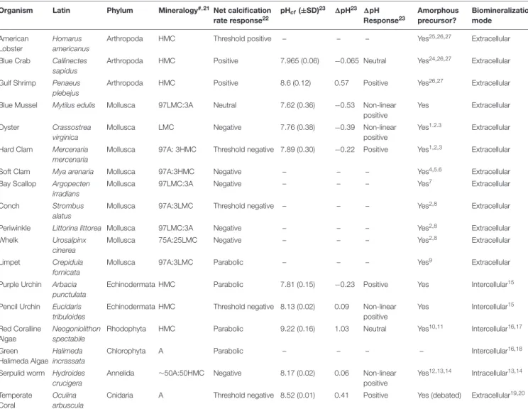
TABLE 1 | Species examined in this study with supporting data.
Organism Latin Phylum Mineralogy#,21Net calcification
rate response22 pHcf(±SD)23 1pH23 1pH Response23 Amorphous precursor? Biomineralization mode American Lobster Homarus americanus
Arthropoda HMC Threshold positive – – – Yes25,26,27 Extracellular
Blue Crab Callinectes sapidus
Arthropoda HMC Positive 7.965 (0.06) −0.065 Neutral Yes24,26,27 Extracellular
Gulf Shrimp Penaeus plebejus
Arthropoda HMC Positive 8.6 (0.12) 0.57 Positive Yes26,27 Extracellular
Blue Mussel Mytilus edulis Mollusca 97LMC:3A Neutral 7.62 (0.36) −0.53 Non-linear positive
Yes Extracellular Oyster Crassostrea
virginica
Mollusca LMC Negative 7.76 (0.38) −0.39 Non-linear
positive
Yes1.2.3 Extracellular Hard Clam Mercenaria
mercenaria
Mollusca 97A: 3HMC Threshold negative 7.89 (0.30) −0.22 Positive Yes1,2,3 Extracellular
Soft Clam Mya arenaria Mollusca 97A:3HMC Negative – – – Yes4,5.6 Extracellular
Bay Scallop Argopecten irradians
Mollusca 97LMC:3A Negative – – – Yes7 Extracellular
Conch Strombus
alatus
Mollusca 97A:3LMC Threshold negative – – – Yes2,8 Extracellular
Periwinkle Littorina littorea Mollusca 97LMC:3A Negative – – – Yes2,8 Extracellular
Whelk Urosalpinx
cinerea
Mollusca 75A:25LMC Negative – – – Yes2,8 Extracellular
Limpet Crepidula fornicata
Mollusca 97A:3LMC Parabolic – – – Yes9 Extracellular
Purple Urchin Arbacia punctulata
Echinodermata HMC Parabolic 7.81 (0.15) −0.23 Positive Yes Intercellular15
Pencil Urchin Eucidaris tribuloides
Echinodermata HMC Threshold negative 8.13 (0.02) 0.09 Non-linear positive Yes Intercellular15 Red Coralline Algae Neogoniolithon spectabile
Rhodophyta HMC Parabolic 9.22 (0.16) 1.03 Neutral Yes10,11 Intercellular16,17 Green
Halimeda Algae Halimeda incrassata
Chlorophyta A Parabolic – – – – Intercellular16,18
Serpulid worm Hydroides crucigera
Annelida ∼50A:50HMC Negative 8.17 (0.02) 0.06 Non-linear positive Yes12,13,14 Intracellular13,14 Temperate Coral Oculina arbuscula
Cnidaria A Threshold negative 8.52 (0.01) 0.41 Positive Yes (debated) Extracellular19,20
#High Mg-calcite (HMC), low Mg-calcite (LMC), aragonite (A); mineralogy is considered mixed if the proportions exceed a 90:10 split; otherwise, if less, the biomineral is
considered to be called the dominant mineral [e.g., 97A:3LMC is considered to be A in the following analyses as the detection limit for the XRD used inRies (2011)as 3%]. More specific quantification regarding relative proportions of each mineralogy can be found inRies, 2011;1Weiss et al., 2002;2Addadi et al., 2006;3Immenhauser et al., 2016;4Harper et al., 1997;5Gazeau et al., 2013;6Meseck et al., 2018;7Brecevic and Nielsen, 1989;8Nassif et al., 2005;9Heinemann et al., 2011;10Leptophytum
foecundum;Rahman et al., 2019;11Corallina elongate;Raz et al., 2000;12De Yoreo et al., 2015;13Chan et al., 2015a;14Chan et al., 2015b;15Wilt, 2002;16Halimeda
sp.;Cuif et al., 2013;17Borowitzka and Larkum, 1987;18Halimeda;Wilbur et al., 1969;19Constantz, 1986;20Constantz and Meike, 1989;21Ries, 2011;22Ries et al., 2009;23Liu et al., 2020;24Dillaman et al., 2005;25Mergelsberg et al., 2019;26Luquet, 2012;27Roer and Dillaman, 1984.
tropical pencil urchin (Eucidaris tribuloides), serpulid worm (Hydroides crucigera), temperate coral (Oculina arbuscula), American oyster (Crassostrea virginica), bay scallop (Argopecten irradians), blue mussel (M. edulis), hard clam (Mercenaria mercenaria), and soft clam (Mya arenaria; see Table 1 for details). Calcium carbonate powders were collected by scraping the growing edge of shells or skeletons (e.g., molluscs, corals, algae, and serpulid worms), by sampling the tip of individual spines (e.g., urchins), or by pulverizing and homogenizing the entire carapace if it was formed entirely under the experimental conditions (e.g., crabs, lobster, and shrimp). Shell or skeleton formed exclusively under the experimental conditions was identified relative to a 137Ba spike that was emplaced in the
shells/skeletons at the start of the experiment (Ries, 2011).
Measurement of Element/Calcium Ratios
Element/calcium ratios were determined for all taxa (Supplementary Table 3) via inductively coupled plasma atomic emission spectrophotometry (ICP-AES). Samples were first cleaned to remove organic matter using an oxidative procedure described in Barker et al. (2003)for the analysis of foraminiferal samples. The sample set contains a number of biomaterials from taxa that have seldom or never been analyzed for X/Ca ratios, including the crustacean carapace, which is a complex biomineral containing chitin and with variable carbonate content. Given the compositional complexity and diversity of the sample set, it was not practical to optimize the cleaning and sample preparation protocol for each species, including assessing potential matrix effects for every species, as
this would have been prohibitively costly in terms of time and financial resources. Instead, we used the established protocol of Barker et al. (2003) that is widely used for trace element determinations within biogenic carbonates (e.g.,Yu et al., 2005).
Calcium concentrations and X/Ca ratios were determined using a Varian Vista ICP-AES at the University of Cambridge, following the methods of de Villiers et al. (2002) and Barker et al. (2003). Pursuant to the procedures outlined in these studies, samples were diluted to be matrix-matched with standards at a Ca2+ concentration of 60 ppm and analyzed in duplicate for consistency. The relative standard deviation (%RSD) of repeated analyses of standards and samples was better than 0.2% for Mg/Ca, consistent withBarker et al. (2003).
All samples were then analyzed on a PerkinElmer Elan DRC II quadrupole inductively coupled plasma mass spectrometer at the University of Cambridge to determine Li/Ca, B/Ca, Zn/Ca, Sr/Ca, Cd/Ca, Ba/Ca, U/Ca, and Na/Ca ratios, with the exception of the crustacea (crabs, lobsters, and shrimp) andHalimeda algae due to issues with nebulizer blockage or because elemental ratios were outside of the working range established by the standards. An intensity-ratio calibration was used for determinations, following the procedure ofYu et al. (2005). The relative standard deviation (%RSD) of repeat analyses of standards and samples is better than 1.2% for all elemental ratios, consistent withYu et al. (2005).
Apparent Partition Coefficient and
Inorganic Partition Coefficient Selection
Apparent partition coefficients (Table 2) of the carbonate biominerals were calculated by dividing the measured calcium ratios by established corresponding element-to-calcium ratios of seawater (Bruland, 1983), such that:
KX= (X/Ca)(X/Ca)mineral seawater
(1) Inorganic elemental partition coefficients for comparison to biominerals were selected from inorganic calcite or aragonite precipitation studies (See Table 2 and Supplementary Table 6) that employed experimental conditions similar to the culturing experiment of Ries et al. (2009). The inorganic precipitation experiments included in this comparison generally used filtered or artificial seawater and were conducted at or near 25◦
C and within a pHsw range of 7.2–8.5. A summary of the
selected partition coefficients for synthetic aragonite, calcite, and amorphous calcium carbonate are presented in Table 2 (see more detailed descriptions of experimental conditions in
Supplementary Table 6 and a more detailed review of the literature on element partitioning between inorganic CaCO3
and fluid in Supplementary Material section “Description of Inorganic Partition Coefficient Selection”).
Statistics
All statistical analyses were conducted in R version 3.6.2 (R Core Team, 2019). Outlier testing was conducted using Rosner’s Test as implemented in the EnviroStat R package (v0.4-2, Le et al., 2015). This test was used because it was designed to avoid masking effects, which are losses in test power due to larger
numbers of outliers being present than being tested for. Outliers were not considered in the analyses and are not illustrated in plots. A complete spreadsheet of the raw data is provided as
Supplementary Data Sheet 2.
Models and Akaike Information Criterion (AIC)
Models relating X/Ca ratios to seawater carbonate parameters (pHsw, [CO32−]sw), net calcification rates (Ries et al., 2009), and
boron isotope derived pHcf (Liu et al., 2020) were conducted
by fitting both linear and quadratic models to the data. Both the linear and quadratic models only include sums of terms; thus, both types of models can be considered linear regressions, evaluated, and compared. The regressions were conducted using the glm function in base R, which returned R2 values and F-test statistics. Since both linear and quadratic
models were considered linear regressions,R2values associated with the regression analyses were comparable and used to model the relationship between the tested variables. The F-test within the glm function is a test of overall significance that compares the specified model to a model with no predictors and subsequently generates a p-value. Regression models that returned a p-value < 0.05 were considered to indicate a statistically significant relationship between the variables of interest. Scatterplots were generated using the ggplot2, ggtext, andRmisc packages in R and are displayed in Supplementary
Figures 10–45(v3.32,Wickham, 2016; v0.1.1,Wilke, 2020; v1.5,
Hope, 2013). Modeled relationships with ap-value< 0.05 were outlined in red (Supplementary Figures 10–45). The code used to generate the plots is available on Github with links provided in
Supplementary Materialsection “Phylogenetic Analysis.” Akaike information criterion (AIC), which ranks models based on their fit and parsimony (Anderson and Burnham, 2004), was used to select between linear or quadratic models for the data. The AIC model that returned the smallest AIC score was selected as the optimal model for describing the relationship between the X/Ca ratio and carbonate chemistry or other measured parameter. The results of the AIC tests are summarized in
Tables 3–5, which show the adjusted R2 and p-values for all species exhibiting statistically significant relationships.
Generalized Additive Models (GAMs)
We modeled the relationships between eight X/Ca ratios and Mg/Ca ratios using generalized additive models (GAMs) from the mgcv package (v1.8–31, Marra and Wood, 2011; Wood, 2017). GAMs are an extension of the generalized linear model family, with the benefit that they have no assumption of a linear relationship between the predictor and response variables, and no assumption of a specific underlying distribution in the data (Hastie and Tibshirani, 1990). Smoothing parameters (penalized regression splines) are introduced and automatically calculated via generalized cross validation (GCV) in the GAM implementation in mgcv (Wood, 2011). GAMs are frequently employed in ecological and environmental contexts where the nature of the relationship between predictors and responses is not known a priori, and/or a flexible nonparametric model is required.
fe art-09-641760 April 28, 2021 T ime: 17:15 # 6 Ulrich et al. Elemental Ratios Recapitulate Phylogeny
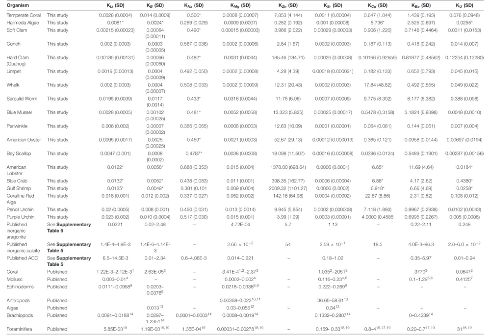
TABLE 2 | Summary of partition coefficients, including calculated apparent partition coefficients of the species cultured in this study; imputed values; synthetic calcite, aragonite, and amorphous calcium carbonate (ACC); and a number of published biogenic apparent partition coefficients.
Organism KLi(SD) KB(SD) KNa(SD) KMg(SD) KZn(SD) KSr(SD) KCd(SD) KBa(SD) KU(SD)
Temperate Coral This study 0.0028 (0.0004) 0.014 (0.0009) 0.506* 0.0008 (0.00007) 7.853 (4.144) 0.0011 (0.00004) 0.647 (1.044) 1.439 (0.195) 0.676 (0.0948) Halimeda Algae This study 0.0081* 0.0024* 0.259 (0.029) 0.0009 (0.0007) 0.252 (0.192) 0.001 (0.00008) 5.736* 2.525 (0.697) 0.0255* Soft Clam This study 0.00215 (0.00023) 0.00064
(0.00011)
0.490* 0.00015 (0.00003) 3.966 (2.022) 0.00029 (0.00003) 0.906 (1.220) 0.7146 (0.4464) 0.0311 (0.0153)
Conch This study 0.002 (0.0003) 0.0003
(0.00005) 0.567 (0.038) 0.0002 (0.00006) 2.84 (1.67) 0.0002 (0.00003) 0.187 (0.113) 0.418 (0.242) 0.014 (0.007) Hard Clam (Quahog) This study 0.00185 (0.00131) 0.00066 (0.00050) 0.482* 0.0031 (0.0044) 185.46 (184.71) 0.00026 (0.00008) 0.10166 (0.92659) 0.81877 (0.48562) 0.12254 (0.13280)
Limpet This study 0.0019 (0.00013) 0.0004
(0.00009)
0.492 (0.050) 0.0002 (0.00008) 4.28 (4.39) 0.00018 (0.000021) 0.182 (0.133) 0.652 (0.793) 0.045 (0.015)
Whelk This study 0.002 (0.0003) 0.0004
(0.00007)
0.508 (0.033) 0.0002 (0.00009) 12.31 (20.43) 0.0002 (0.00003) 17.84 (48.82) 0.492 (0.555) 0.049 (0.022) Serpulid Worm This study 0.0195 (0.0039) 0.0117
(0.0014)
0.433* 0.0316 (0.0044) 11.75 (6.06) 0.0007 (0.00009) 9.775 (8.302) 8.177 (6.382) 0.388 (0.098) Blue Mussel This study 0.0028 (0.0005) 0.00102
(0.00025)
0.481* 0.0052 (0.0058) 13.323 (5.825) 0.00025 (0.00017) 0.5478 (0.3158) 3.1824 (6.9398) 0.0048 (0.0010)
Periwinkle This study 0.006 (0.002) 0.00007
(0.00002)
0.366 (0.065) 0.0008 (0.0003) 12.63 (10.09) 0.0001 (0.00001) 0.064 (0.061) 0.144 (0.051) 0.007 (0.004) American Oyster This study 0.0095 (0.0017) 0.0025
(0.00025)
0.459* 0.0021 (0.0003) 52.67 (29.13) 0.00012 (0.000013) 0.365 (0.121) 0.0958 (0.0144) 0.00697 (0.0194) Bay Scallop This study 0.0047 (0.001) 0.0008
(0.0002)
0.4787* 0.0038 (0.0008) 18.098 (11.507) 0.00016 (0.000008) 0.0396 (0.0124) 0.5489 (0.1901) 0.00287 (0.00156) American
Lobster
This study 0.0122* 0.0058* 0.688 (0.353) 0.015 (0.004) 1378.00 (698.64) 0.0006 (0.0001) 6.65* 11.69 (4.64) 0.0184*
Blue Crab This study 0.0132* 0.0052* 0.438 (0.083) 0.011 (0.001) 398.35 (162.77) 0.0006 (0.00004) 6.88* 4.17 (2.62) 0.4380*
Gulf Shrimp This study 0.0125* 0.0049* 0.381 (0.101 0.009 (0.004) 2009.32 (1101.27) 0.0006 (0.0002) 6.918* 6.66 (4.69) 0.0258*
Coralline Red Alga
This study 0.018 (0.001) 0.012 (0.002) 0.337 (0.027) 0.052 (0.002) 142.16 (64.98) 0.0004 (0.00002) 22.87 (8.86) 2.31 (0.52) 0.108 (0.012) Pencil Urchin This study 0.02 (0.0005) 0.008 (0.001) 0.450 (0.031) 0.013 (0.0014) 9.945 (5.854) 0.0002 (0.000008) 7.118 (1.893) 0.9967 (0.2938) 0.0102 (0.0043) Purple Urchin This study 0.023 (0.002) 0.010 (0.0004) 0.517 (0.030) 0.015 (0.001) 3.99 (1.99) 0.0003 (0.00001) 4.0000 (0.4585 0.6995 (0.2267) 0.005 (0.0008) Published inorganic aragonite See Supplementary Table 5 0.0321 0.02–2.48 – 4.72E-04 5.7 1.13 – 0.22–2.11 0.248 Published inorganic calcite See Supplementary Table 5 1.4E-4–4.9E-3 1.4E-6–4.14E-3 – 2.66 × 10⁻² 54 2.59 × 10⁻¹ 18.5 4.0E-3–96.3 2.0–6.0 × 10⁻²
Published ACC See Supplementary Table 5
6.5–14.5E-3 0.01–2.34 0.6–4.06E-3 0.014–0.221 – 0.18–1.02 – 0.35–5.97 0.01–0.94
Coral Published 1.22E-3–2.12E-31 2.63E-052 – 3.41E-41,2–2.373 1.0352–20513 37703 0.06472
Mollusc Published 0.003–0.014 – – 0.0002–0.0024 – 0.116–0.234,6 – 0.1–1.295,6 0.41257 Echinoderms Published 0.0111–0.09589 0.0203– 0.03769 – 0.0218–0.03388,9 – 0.222–0.2698 – – – Arthropods Published 0.00358–0.02210,11 36.65–58.6110 Algae Published 0.01313 – 0.03–0.05512 – 0.3412 – – – Brachiopods Published 0.0091–0.018814 0.0297– 1.235114 0.0001–0.000314 0.0008–0.001914 0.1332–0.280714 0–0.423914
Foraminifera Published 5.85E-0319 1.19E-0315,19 1.35E-0419 0.00031–0.0027818,19 – 0.159- 0.3318,19 0.8–415,17,19 0.20–0.717,19 3116,19 1Montagna et al., 2014;2Sinclair and Risk, 2006(model);3Gaetani et al., 2011(model);4Calculated fromDellinger et al., 2018;5Gillikin et al., 2006;6Zacherl et al., 2003;7Frieder et al., 2014;8Lavigne et al., 2013; 9Nguyen, 2013;10Wickins, 1984;11Kondo et al., 2005;12Ries, 2006;13Donald et al., 2017;14Jurikova et al., 2020;15Dang et al., 2019;16Keul et al., 2013;17Havach et al., 2001;18Raitzsch et al., 2010;19Allen et al., 2016. *Refers to the apparent partition coefficients that were calculated using imputed values.
Fr ontiers in Earth Science | www .fr ontiersin.org 6 May 2021 | V olume 9 | Article 641760
We tested models with and without the presence of the variable “Phylum” as both an additive and interactive effect to better explore the influence of taxonomy on mineralogy. It should be noted that these analyses are distinct from the phylogenetic analyses described below in section “Phylogenetic Analyses,” as they are not informed by the phylogenetic relationships between species. Models were fit using maximum likelihood, and a likelihood ratio test from packagelmtest (v0.9–38,Zeileis and Hothorn, 2002) was used to select from among candidate models. In cases where the likelihood ratio test indicated that two models were equally likely, we selected the less complex model. Each final model fit was bootstrapped using 1,000 iterations in package boot (v1.3–25, Davison and Hinkley, 1997; Canty and Ripley, 2020) to produce a more robust estimate of theR2 and is accompanied by a 95% confidence interval around the bootstrappedR2 (Supplementary Tables 4, 5; see Table 6 for a summary of the best-performing models).
Imputation, Hierarchical Clustering, and Ordination
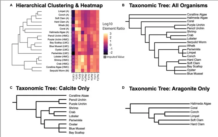
A K-Nearest-Neighbors (KNN) machine learning algorithm was employed to estimate missing values (with a pseudocount of +1 added to place the values on a log-10 scale) in the X/Ca ratio dataset (14.21% of the dataset) using theimpute R package (v1.64.0,Beretta and Santaniello, 2016;Hastie et al., 2020). For this model, KNN selects ana priori neighborhood (3 in this study to get a range of values and not overfit value estimation) and imputes them using a weighted mean of the neighbors where those with the smallest Euclidean distance have more impact on the final estimation. Each “object” represents a species, and its location in the space is determined by each of the log-10 transformed X/Ca ratios. The distance between objects is their straight-line distance in the space. The analysis begins by treating each organism as a separate cluster. Then, the algorithm iteratively merges the two closest (i.e., most similar) clusters until all are merged. The main output of the hierarchical clustering analysis is the dendrogram on the left of Figure 4, which shows the results of the iterative clustering and reveals relationships in X/Ca ratios separated by mineralogy (Figure 4). The resulting dataset was used for ordination and cluster analysis.
Clustering and ordination of elemental ratios by taxon and annotation of phylum was conducted using the vegan and ggplot2 packages (v3.32,Oksanen et al., 2008; v2.5–7,Wickham, 2009). Bray-Curtis dissimilarity (a statistic used to quantify the compositional dissimilarity between two different sites) was calculated for each pairwise imputed elemental ratio by species and subject to complete linkage hierarchical clustering, where the maximum distance between two clusters is identified and the new clusters are merged. This step is repeated until the dataset has agglomerated into a complete dendrogram. The same values were used to model species dissimilarity in ordination space using Non-metric Multidimensional Scaling (NMDS), which was selected because it is rank-based and detects non-linear relationships well. The model collapses information from multiple dimensions and projects this into a lower state (2 dimensions) and iteratively (999 iterations) places objects in ordination space while minimizing distance in projected dimensions as compared to the original dissimilarity matrix.
Phylogenetic Analyses
Initial phylogenetic trees reflecting the taxonomy for the invertebrate species studied here was constructed with the phyloT application1 based on the NCBI taxonomic backbone
(Figures 4B–D). NCBI taxonomy IDs used for the studied species were 6706 (H. americanus), 6763 (C. sapidus), 161926 (P. plebejus), 6550 (M. edulis), 6565 (C. virginica), 6596 (M. mercenaria), 6604 (M. arenaria), 31199 (A. irradians), 387448 (S. alatus), 31216 (L. littorea), 399971 (U. cinerea), 176853 (C. fornicata), 7641 (A. punctulata), 7632 (E. tribuloides), 2071691 (Neogoniolithon sp.), 170419 (H. incrassata), 1196087 (H. crucigera), and 1282862 (O. arbuscula). This tree constructed using the NCBI taxonomy was used to initially examine the correlation of species’ geochemistry and mineralogy against taxonomy.
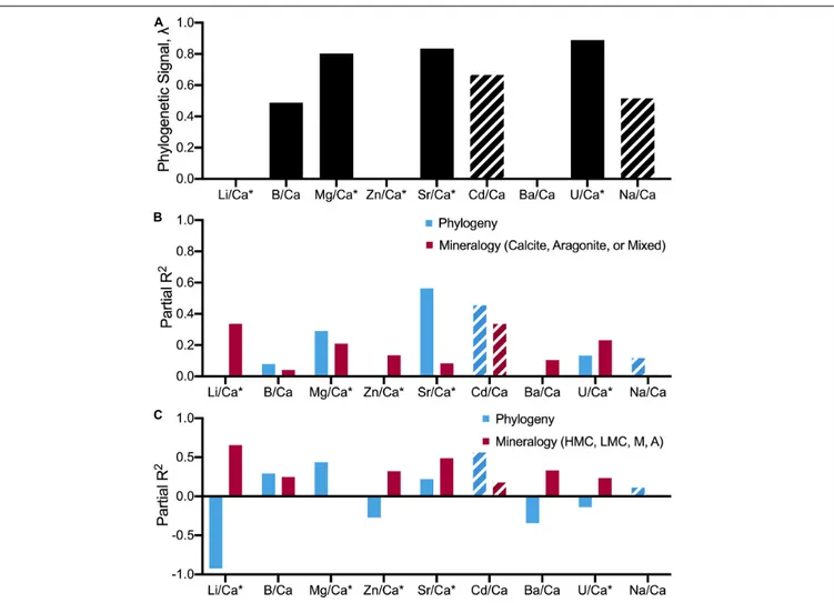
Next, two mitochondrial (COI, cytb) gene regions and a single nuclear (18S) gene region were used to infer the phylogenetic relationships and times of divergence for all the 18 focal species. Supplementary Material section “Methods and Results of Phylogenetic Trees” includes details on tree assembly in BEAST 1.10 (Suchard et al., 2018). The resulting phylogeny is provided in Supplementary Material section “Link to Nexus File for Time-Calibrated Phylogenetic Tree.” The newly assembled time-calibrated phylogeny was first used to test for phylogenetic signal in geochemistry. Phylogenetic signal, defined as the tendency for closely related species to resemble each other more than species selected at random from the tree, is here used as a test for phylogenetic conservatism or inertia in geochemistry (Pagel, 1999). However, the coupling between evolutionary history and patterns of X/Ca divergence between species can also be confounded by alternative variables such as mineralogy (Table 7). Thus, regression models incorporating the newly inferred phylogeny were used to estimate the relative contributions of mineralogy and evolutionary history to differences in geochemistry among species (Figure 5).
Phylogenetic signals in the elemental geochemistry were estimated using both uni- and multivariate approaches. The univariate phylogenetic signal (i.e., for each elemental ratio) was computed using the lambda statistics in the phylosig function in thephytools R package (v0.7–70,Revell, 2012). Next, multivariate phylogenetic signals (i.e., across all elemental ratios) were estimated with Pagel’s lambda (Pagel, 1999) using the phyl.pca inphytools (Revell, 2009, 2012). For both approaches, lambda estimates range from 0 to 1, with values closer to 1 indicating that differences in elemental ratio(s) among species reflect evolutionary history (phylogenetic conservatism). Finally, the initial dataset was partitioned into five different datasets with variable number of imputed values to determine whether they affect the resulting phylogenetic signal (see details in
Supplementary Table 9). First, the phylogenetic signal of an elemental dataset, including all of the elements except Cd/Ca and Na/Ca Second, the original dataset was subsampled for only Zn/Ca, Mg/Ca, Sr/Ca, and Li/Ca data. This dataset did not include any imputed values. Third, since almost half of elemental data for the arthropods were imputed, the shrimp,
feart-09-641760 April 28, 2021 Time: 17:15 # 8
Ulrich et al. Elemental Ratios Recapitulate Phylogeny
crabs, and lobsters were excluded from the analyses. Fourth, a dataset with all species was generated that included only Mg/Ca and Sr/Ca data. Fifth, a dataset of all species was generated that included only Mg/Ca, Sr/Ca, and Li/Ca. This set of five additional datasets was used to examine the effects of data imputation on the multivariate phylogenetic signal estimate. Lastly, the relative contributions of the phylogeny and mineralogy to geochemistry patterns among species was estimated using phylogenetic and non-phylogenetic regression models. It should be noted that patterns of divergence between X/Ca ratios and phylogenetic signal can still be explained by differences in polymorph mineralogy. Thus, a set of three regression models were fit for each of the elemental ratios. Each set of regression models included an intercept-only linear regression model (model 1), a linear regression model between the target elemental ratios and mineralogy (model 2), and a phylogenetic regression model between the target elemental ratios and mineralogy (model 3). Non-phylogenetic models were fit using the lm function in the stats R package. Phylogenetic regression models, with lambda values estimated from the data, were fit using the phylolm function in the phylolm R package (v2.6.2; Ho et al., 2016). The relative contribution of differences in biogenic carbonate mineralogies among species to elemental ratios among species was estimated by comparing partial R2-values between non-phylogenetic models (models 1 and 2). Similarly, the relative contribution of evolutionary history to explaining differences in elemental ratios among species was estimated by comparing partial R2-values between
the phylogenetic regression and the linear regression models of elemental ratios versus mineralogy across species and pCO2
conditions (models 2 and 3). Comparison of partialR2-values, following Ives (2018), was conducted using the rr2 R package (v1.0.2,Ives and Li, 2018).
RESULTS
The reported X/Ca ratios for each species represent means of the measured data across the pCO2 culture conditions
(Supplementary Table 3). These mean values were used for the multivariate and phylogenetic analyses described below because the range of X/Ca values for a given species across pCO2treatments is relatively small compared to the differences
in mean X/Ca of different species. For example, the pencil urchin, E. tribuloides, exhibits Li/Ca and Mg/Ca values of 50– 53 µmol/mol and 60–78 mmol/mol across pCO2 treatments,
respectively, whereas the oyster, C. virginica, exhibits values of 15–30µmol/mol and 9.5–13 mmol/mol, respectively (Figure 1).
Element/Calcium Ratios Amongst
Diverse Marine Calcifiers
As expected, Mg, Sr, and Na were the most abundant elemental substitutions across all mineralogies (Figure 1 and
Supplementary Table 3;Reeder, 1983;Sugawara and Kato, 2000;
Allison et al., 2001; Iglikowska et al., 2016). The calcite in crustaceans’ carapaces and urchins’ spicules exhibits Mg/Ca in the range of 50–100 mmol/mol and the mixed mineralogy serpulid
worm and calcitic coralline red algae exhibit relatively high Mg/Ca in the range of 100–300 mmol/mol, while the aragonite-producing species were low in Mg/Ca. Molluscs exhibited low Mg/Ca, regardless of the CaCO3 polymorph produced. Sr/Ca
was highest in the range of 9–12 mmol/mol in the aragonite-forming coral and green algae. Strikingly, mollusc CaCO3of all
polymorphs was relatively low in all elemental ratios compared to other species, except for Li/Ca compared to the temperate coral and Na/Ca compared to most other species. Of the other elements, Li/Ca and B/Ca was notably higher in organisms that formed high-Mg calcite, including the serpulid worm, which produces a worm tube of aragonite and high-Mg calcite (see more analyses below in section “Relationships Between Mg/Ca and Other Elemental Ratios”). B/Ca was also high in the aragonite coral skeleton. The coralline red algae and serpulid worm generally had comparatively high levels of all measured elements compared to the other species. Amongst the aragonite producing species, the coral was noticeably different in that it exhibited much higher B/Ca, Sr/Ca, and U/Ca. The Halimeda algae exhibited elemental ratios similar to those of the coral.
Relationships Between Mg/Ca and Other
Elemental Ratios
Generally, higher incorporation of Mg in the biomineral lattice appears to be linked to higher incorporation of other elements (Figure 2). For example, for Li/Ca, the molluscs and coral group together with lower Mg content (Li/Ca: 6.5–25µmol/mol; Mg/Ca: 0.5–6 mmol/mol), while the echinoderms, serpulid worms, and coralline red algae are relatively enriched in both Mg and Li (Li/Ca: 39–60µmol/mol; Mg/Ca: 60–275 mmol/mol). Potential increases in Zn/Ca with Mg incorporation are less clearly resolved.
In this X/Ca-Mg/Ca space, the data appear to group by phylum, so generalized additive models (GAMs) were used to explore the influences of phylum and mineralogy on elemental clustering. The final GAMs explain between 26.4 and 99% of the variation in the elemental ratio of interest, with model selection indicating a preferred final model with phylum, or a combination of phylum and mineralogy, for seven of the eight elements (see Table 6 for final models; see Supplementary Table 4 for complete list of candidate models; see in Supplementary Table 5 for likelihood ratio test results; see Supplementary Figure 9 for final model components). Models that only consider Mg/Ca explain up to 71.9% of the variation in the element of interest but were in no case preferred by model selection. In seven of eight cases, including mineralogy with Mg/Ca substantially improves the models and explains between 16.6 and 95.6% of the variation in the element of interest. Cd/Ca is the only case where the model including only mineralogy was preferred. Six of the eight models were improved by including phylum, explaining up to 98.7% of the variation. All final models produced normally distributed residuals (Supplementary Figures 1–8). Overall, we find evidence that both mineralogy and phylum are key predictors of elemental ratios in the study organisms. Please note that these models consider the phylum that were used to classify the samples (i.e., Rhodophyta, Chlorophyta,
FIGURE 1 | Elemental ratio data across all pCO2 culture conditions combined for the invertebrates studied. Color and shape indicate phylum and mineralogy, respectively. The species are organized from left to right according to mineralogy: Aragonite, Mixed Mineralogy, and Calcite. Mixed Mineralogy refers to carbonates with less than 90% of either aragonite or calcite. Differences between species and phyla are typically much greater than the variation within species data that could be attributed to varying seawater conditions. Note some elemental ratios are not displayed to avoid scale compression or due to low confidence in their analytical accuracy (e.g., arthropod Zn/Ca; see section “Materials and Methods”).
Cnidaria, etc.); the models are not informed by the phylogenetic relationships between species. The results of the phylogenetically informed analyses are described below in section “Phylogenetic Signal and Regression Analyses.”
Comparison of Inorganic Carbonate
Element Partitioning to Marine
Biominerals
Patterns of elemental partition coefficients (Kx) observed here
are of course similar to those observed for the X/Ca data. However, calculating the apparent partition coefficients allows for comparison to other cultured biogenic samples and published
partition coefficients derived from inorganic synthesis of calcite, aragonite, and amorphous calcium carbonate (ACC; Table 2 and Figure 3). Though some apparent partition coefficients align with those of inorganically precipitated CaCO3 minerals
(e.g., KLi for aragonitic organisms and ACC; KLi for calcitic
organisms and calcite), there are many that are relatively enriched or depleted with respect to those observed for inorganic precipitates. Positioning relative to the inorganic partition coefficients appears to be consistent amongst organisms of the same phylum regardless of mineralogy, as observed, for example, in the mollusca.
The molluscs are relatively depleted with respect to most of the measured elements compared the other organisms,
feart-09-641760 April 28, 2021 Time: 17:15 # 10
Ulrich et al. Elemental Ratios Recapitulate Phylogeny
FIGURE 2 | Elemental ratio data plotted against Mg/Ca (log10-transformed values are shown. Color and shape indicate phylum and mineralogy, respectively. Generalized additive models (GAMs) of this data show a number of significant relationships between elemental ratios and Mg/Ca, explaining 0–71% of the variance in the data (Supplementary Table 4). Grouping the organisms by phylum or mineralogy substantially improves model performance, and the best-performing models consider either or both grouping variables (38.70–99.00% of variance explained; Table 6).
while the coralline red algae and echinoderms are relatively enriched with respect to these elements. For KLi, the coral
and the molluscs, regardless of mineralogy, exhibited values aligned with the published inorganic partition coefficients of ACC. The apparent KB values of the calcitic organisms all
lie closest to the published partition coefficient for calcite (Figure 3 and Table 2). The apparent KB of aragonitic coral
(0.014 ± 0.0009) is depleted relative to inorganic aragonite (0.02–2.48). The apparent KB of the serpulid worm tube
(0.0117 ± 0.0014) falls between the published values for inorganic calcite (1.4E-6-4.14E-3) and inorganic aragonite (0.02–2.48), consistent with its mixed mineralogy.
KZnvalues spanned the greatest range across the organisms,
with the crustaceans exhibiting values>200. Only the coralline red algae exhibited KZn that was comparable to that of the
crustacea, ranging from approximately 100 to 200. With the exception of the calcitic Eastern Oyster, which has an apparent partition coefficient similar to that of inorganic calcite, the remainder of the organisms sampled align with theKZnpublished
for inorganic aragonite.
Surprisingly, apparent KSr for all species studied were
lower relative to published values for inorganic precipitates of corresponding carbonate polymorph (Schöne et al., 2010). The highest apparent KSr for organisms were calculated
FIGURE 3 | Heatmaps displaying the log10-transformed differences between apparent partition coefficients and published partition coefficients from inorganic mineral precipitation experiments (See Table 2 for values; Supplementary Table 5 for experimental conditions and citations for inorganic values). The apparent elemental partition coefficients calculated for the cultured species studied typically do not align with values derived from synthetic minerals, and species belonging to the same phyla appear to exhibit similar patterns. The warm color gradient (i.e., the left, yellow-black gradient) represents when biogenic carbonates are enriched in an element relative to the published synthetic values (KSynthetic< KBiogenic). Alternatively, a green-yellow color gradient (i.e., the right gradient) represents when biogenic carbonates are depleted relative to the published synthetic values (KBiogenic< KSynthetic). White pixels indicate that no published, synthetic values for that element were found. Circles within pixels denote imputed values (See section “Imputation, Hierarchical Clustering, and Ordination” and Figure 4 for details). Apparent partition coefficients were calculated by dividing the measured and imputed elemental ratios of the biogenic carbonates by established seawater minor and trace element concentrations (Bruland, 1983). The top row of panels presents the aragonitic organisms, while the bottom panels represent the calcitic organisms. The label above each panel denotes the inorganic, synthetic partition coefficients being compared to (i.e., aragonite, calcite, and amorphous calcium carbonate; ACC). The color of the pixels was determined by log10(| KX, Biogenic – KX, Synthetic|). The absolute value is used since y cannot be less than 0 in log10(y).
from the aragonitic species of coral and Halimeda algae sampled, which range from 0.001 to 0.00125. The next highest values were calculated for the serpulid worm and the arthropods—approximately half of that of the aragonite species—which possess shells of mixed mineralogy and high-Mg calcite, respectively. The KSr of the coralline red algae
(4E-4 ± 0.2), molluscs (1.8-2.9E-4), and echinoderms (2.0-3.0E-4) are even lower.
All of the molluscs, as well as the aragonitic coral and Halimeda algae, have apparent KMg similar to that of
synthetic aragonite (4.72E-4). The high-Mg calcite arthropods and echinoderms are enriched relative to the values for
published inorganic calcite (2.66E-2), while the serpulid worm is comparable to value for inorganic calcite. Coralline red algae high-Mg calcite exhibits the highestKMgat approximately 0.06.
There were no published partition coefficients for Cd in synthetic aragonite. The publishedKCdfor synthetic calcite (18.5)
overlaps with the highest and lowest ends of the respective ranges of apparentKCd calculated for the serpulid worm (9.78)
and the coralline red algae (22.9). The coral, molluscs and echinoderms are all extremely depleted with respect to Cd relative to synthetic calcite.
The apparentKBavalues calculated for the crustacea and the
feart-09-641760 April 28, 2021 Time: 17:15 # 12
Ulrich et al. Elemental Ratios Recapitulate Phylogeny
partition coefficients for synthetic CaCO3minerals, though their
values range widely from 3 to 20. The lowest limit of this range as well as both theHalimeda and the coralline red algae appear to align with the KBa measured for synthetic ACC.
The echinoderms, which produce high-Mg calcite biominerals, provide an apparent KBa consistent with that derived from
synthetic calcite experiments. The apparentKBaof the mollusc
species appear to be consistent, regardless of mineralogy, and lie between the published KBa values for synthetic calcite and
aragonite. The values calculated for coral fall between the published values for synthetic calcite and ACC.
The highest apparent KU are calculated for the coral and
the serpulid worm, ranging from 0.5 to 0.75 and 0.25 to 0.40, respectively, and are both enriched relative to the publishedKU
values for synthetic ACC, calcite, and aragonite. The molluscs, regardless of mineralogy, and the echinoderms partition U similarly to synthetic calcite, except for the mixed mineralogy hard clam, which has an average calculatedKUsimilar to values
published for synthetic aragonite. Coralline red algae appear to partition U similarly to synthetic ACC.
Imputed Values and Hierarchical
Clustering
Some of the analyzed specimens were missing elemental ratios (14.2% of the dataset). These missing data were imputed using the data of similar points in the space (see Methods 2.5.3 for details; see imputed results in Supplementary Table 3) in order to facilitate multivariate and phylogenetic analysis of the dataset. These mean and imputed values for elemental ratios are used for the hierarchical clustering (Figure 4A) and phylogenetic signal analyses (Table 7 and Supplementary Table 8), as well as for the non-metric multidimensional scaling ordinations (NMDS;
Figures 5, 6A,B) described below.
When compared to the taxonomic trees (Figures 4B–D), the hierarchical clustering results of the elemental ratio data (Figure 4A) appear to recapitulate the mineralogically specific taxonomic trees (Figures 4C,D). When including species of differing polymorph mineralogy, the similarities between the clustering analysis and the taxonomic tree (Figure 4B) seem to be confounded by polymorph mineralogy. Parsing out the confounding effects of mineralogy from the effects of phylogeny is explored below.
Phylogenetic Signal and Regression
Analyses
Uni- and multivariate analyses of phylogenetic signal based on the Pagel’s lambda statistics, reflecting the extent to which closely related species show similar X/Ca ratios, generally indicate a strong coupling between the phylogenetic tree and patterns of elemental ratios between species. While a Pagel’s lambda value of 0 for X/Ca ratios would indicate that closely related species are more likely to differ in X/Ca ratios than distantly related species (Pagel, 1999), the multivariate analyses of all nine X/Ca ratios recovered an estimated lambda of 0.89–0.99 (Table 7; range based on alternative datasets), indicating that closely related species tend to have similar X/Ca ratios. However, patterns of congruent
evolutionary history and X/Ca ratios are not generalizable across all X/Ca ratios. For instance, three out of the nine X/Ca ratios examined in this study had phylogenetically decoupled patterns of change in ratios between species (Li/Ca, Zn/Ca, and Ba/Ca;
Table 7).
We also explored the potential impact of the imputed values on the phylogenetic signal results by determining Pagel’s lambda with subsets of the data that minimize the number of imputed values (e.g., 0.938 for all X/Ca ratios except Cd/Ca and Na/Ca; 0.968 for all species except Arthropods) and found no substantial effects of missing data on estimate of phylogenetic signal (Supplementary Table 9). Furthermore, the impact of using a lower number of X/Ca was assessed through determining Pagel’s lambda using subsets of two, three, and four elemental ratios (Table 7). Pagel’s lambda remains high (0.925 for multivariate phylogenetic signal across Mg/Ca, Sr/Ca; 0.803 for Mg/Ca; 0.835 for Sr/Ca; Table 7). However, when an elemental ratio with no apparent phylogenetic signal is included in the analysis, lambda slightly decreases (0.898; Table 7). Thus, the analyses suggest that for some, but not all, of the examined X/Ca ratios, phylogenetic closeness is potentially a major driver of differences in X/Ca values amongst species.
Further, regression analysis was used to examine whether interspecific differences in X/Ca ratios are better explained by phylogeny or differences in mineralogy. As shown above, phylogenetic signal varies between X/Ca ratios (Table 7), so the effects of phylogenetic history relative to mineralogy are expected to vary amongst elemental ratios. Phylogenetic and non-phylogenetic models were used to resolve the relative contributions of evolutionary history and mineralogy to explaining patterns of X/Ca ratios between species. When classifying mineralogy as calcite, aragonite, or mixed, phylogeny was 1.4–59 times better at explaining variance in X/Ca ratios than mineralogy in five out of the nine X/Ca ratios (i.e., B/Ca, Mg/Ca, Sr/Ca, Cd/Ca, and Na/Ca; Figure 7 and Supplementary
Table 9). However, when mineralogical classification is broken down further (high-Mg calcite, low-Mg calcite, aragonite, and mixed), the amount of variance explained by phylogeny decreases to 1.3–15.7 times better in four out of the nine X/Ca ratios, demonstrating the importance of distinguishing between low-Mg and high-Mg calcites. Also notable is that in all but one of the X/Ca ratios (U/Ca), high phylogenetic signal was coupled with higher explanatory effects of phylogeny relative to mineralogy. Overall, these phylogenetic analyses suggest that elevated phylogenetic signals generally indicate that differences in X/Ca ratios are better explained by phylogenetic closeness, not mineralogy. Thus, the elevated phylogenetic signal recovered across all X/Ca ratios using multivariate analyses reflects the major contributions of phylogeny to generating extant patterns of X/Ca ratios amongst species.
Finally, mollusc elemental data were used to examine the relative contributions of mineralogy and phylogeny to explaining differences in X/Ca ratios between species within the same phylum. Regression analyses were conducted comparing the relative contributions of mineralogy and phylogenetic history using phylogenetic and non-phylogenetic models. The mollusk dataset includes four species assigned to the calcite category,
FIGURE 4 | (A) Hierarchically clustered (Bray-Curtis dissimilarity) heatmap of log10 values of element to calcium ratios separated by species. Letters in ellipses correspond to organism biomineralogy: A, aragonite; HMC, high Mg calcite; LMC, low Mg calcite; and M, mixed. Lighter colors indicate higher values from log10-transformations of elemental ratios, and an “O” on top of a pixel indicates that the value was imputed using a K-Nearest Neighbors model estimation (see section “Materials and Methods” for details). (B–D) Taxonomic trees of the studied organisms based on genetic similarity/difference for all, calcitic, and aragonitic species, respectively. Taxonomic trees were built using the phyloT application based on the NCBI taxonomic backbone (see section “Phylogenetic Analyses”;Letunic and Bork, 2019). Qualitative similarities between the resulting dendrogram of the clustering analysis and the mineral-specific taxonomic trees suggest that taxonomic patterns arise in the elemental ratio measurements but are potentially convoluted by mineralogical effects.
four assigned to the aragonite category, and a single species to the mixed mineralogy category. It should be noted that the limited sample size may compromise the calculations assessing phylogenetic signal at the class level presented below. Regression models run for X/Ca ratios with high phylogenetic signals (B/Ca, Mg/Ca, and Sr/Ca; Table 7) found that for two of the three X/Ca ratios examined within molluscs, phylogenetic history better explains patterns of divergence in X/Ca ratios than mineralogy. Phylogeny is about two times better than mineralogy (partial R2
phylogeny = 0.239 vs. mineralogy = 0.097) in predicting B/Ca.
Similarly, phylogeny explains nearly two times more variance in Mg/Ca than mineralogy (partial R2, phylogeny = 0.60 vs. mineralogy = 0.33). For Sr/Ca, both phylogeny and mineralogy explain a similar fraction of differences in ratios between species (partial R2, phylogeny = 0.632 vs. mineralogy = 0.65). Overall,
results within molluscs for X/Ca ratios with high phylogenetic signal indicate that phylogeny is generally a better predictor of differences in X/Ca ratios between species than mineralogy. Nevertheless, as indicated above, these results were potentially affected by the limited sample size and should be re-examined in future studies including more mollusc species. This analysis of
a mollusc-only dataset reaffirms that, for specific X/Ca with high phylogenetic signal, differences in X/Ca between species largely reflect phylogenetic closeness, not mineralogy.
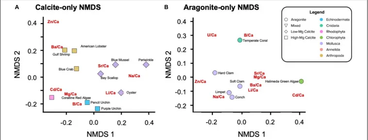
Non-metric Multidimensional Scaling
(NMDS) Ordination
Non-metric Multidimensional Scaling ordinations project the all of X/Ca ratios, including the imputed values, project in two dimensions (Figures 5, 6). As opposed to Euclidean distance, which is the distance computed for the hierarchical clustering analysis, NMDS uses rank-based ordering and is better suited for detecting non-linear relationships. The model iteratively collapses the nine dimensions of X/Ca ratios onto two dimensions, seeking to minimize the distances between species.
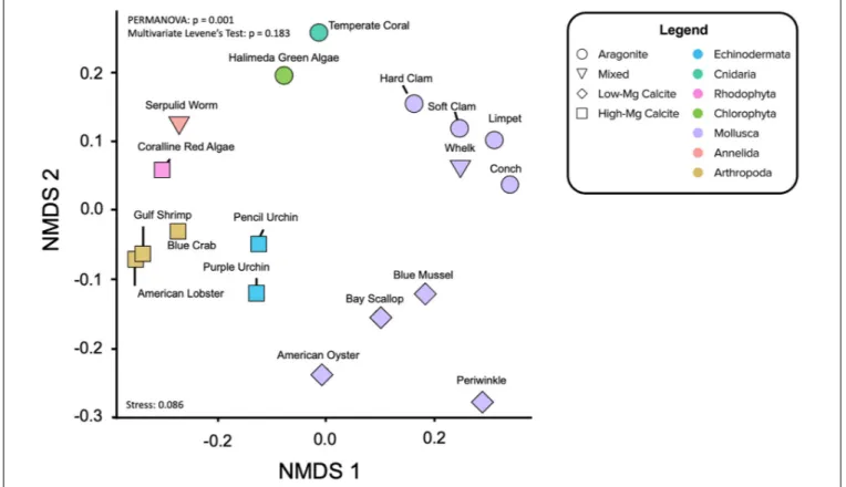
Not surprisingly, there is a split with the dataset between the calcitic and aragonitic organisms, with the 50HMC:50A serpulid worm occupying an intermediate position between the groups (Figure 5). Within mineralogy, however, species cluster according to phylogenetic relationships (Figure 5) much more strongly than in the hierarchical clustering analysis. NMDS
feart-09-641760 April 28, 2021 Time: 17:15 # 14
Ulrich et al. Elemental Ratios Recapitulate Phylogeny
FIGURE 5 | Non-metric Multidimensional Scaling (NMDS) ordination of the elemental ratio data projected to two-dimensions and colored by taxon phylum. Shape denotes mineralogy. PERMANOVA determined whether clustering by phyla is significant (p = 0.001). Multivariate Levene’s test of homogeneity (p = 0.183) and the stress value for this analysis (0.086) are reported. Visualizing the elemental ratio data in this way further illustrates the relative influences of mineralogy and phylogeny and potentially provides a framework for interpreting diagenetic effects of fossil carbonates.
ordination of all organisms shows statistically significant clusters of X/Ca ratios by phylum (i.e., for species of same mineralogy), where the ratios within phylum show equal variances across organisms (PERMANOVA:p = 0.001; permutational multivariate Levene’s test: p = 0.183). For example, the bivalve molluscs fall close together, as do the arthropods and echinoderms. The aragoniticHalimeda green algae and temperature coral aragonitic species lie proximal, as do the high-Mg calcite producing coralline red algae and the serpulid worms of mixed mineralogy.
Separating the calcite-forming (Figure 6A) and the aragonite-forming (Figure 6B) organisms removes the role of mineralogy while revealing rank-based positioning of the X/Ca ratios, themselves. In the calcite-only NMDS, significant clustering of organisms by phylum is also observed (Figure 6A; PERMANOVA: p = 0.003), along with variation within phyla. The X/Ca ratios position themselves in the ordination space with a similar multivariate structure as the organisms; they lie closest to organisms that incorporate them the most. Of the arthropods, Ba/Ca has the most similar data structure to the American lobster and Gulf shrimp. Li/Ca, Na/Ca, and Sr/Ca in the calcitic organisms have data structures similar to those elements in the calcitic molluscs, although there is some variation amongst them. Also, Li/Ca in addition to B/Ca in the calcite ordination to have data structures similar to those elements in the echinoderms. The coralline red alga exhibits the most distinct data structure,
exhibiting high ratios of Mg/Ca, Cd/Ca, and U/Ca. Zn/Ca in the calcite ordination does not appear to have a data structure similar to that of any of the other calcitic organisms. In the aragonite-only NMDS, significant clustering by phyla is again observed (Figure 6B; PERMANOVA:p = 0.136). The temperate coral and the Halimeda green algae have data structures more similar to B/Ca and Cd/Ca, respectively. The aragonitic molluscs, with the exception of the hard clam, exhibit relatively high Na/Ca, Li/Ca, and Ba/Ca. Also of note is the clustering of Sr/Ca, Mg/Ca, Ba/Ca, and Li/Ca for the aragonitic species, potentially indicating similar mechanisms of partitioning.
Relationships Between Elemental Ratios,
Carbonate Chemistry, and Other
Measured Parameters
Relationships between the elemental data and a number of the measured experimental parameters were explored via linear and quadratic regressional analysis, including net calcification rate (Ries et al., 2009), culture water carbonate ion concentration ([CO32−]), culture seawater pH (pHsw), and
δ11B-derived internal calcifying fluid pH (pH
cf;Liu et al., 2020;
Supplementary Figures 10–45). If both linear and quadratic fits were significant, Akaike Information Criterion (AIC) was used to compare and identify the best fit (Tables 3–5).