HAL Id: hal-00304773
https://hal.archives-ouvertes.fr/hal-00304773
Submitted on 1 Jan 2003HAL is a multi-disciplinary open access archive for the deposit and dissemination of sci-entific research documents, whether they are pub-lished or not. The documents may come from teaching and research institutions in France or
L’archive ouverte pluridisciplinaire HAL, est destinée au dépôt et à la diffusion de documents scientifiques de niveau recherche, publiés ou non, émanant des établissements d’enseignement et de recherche français ou étrangers, des laboratoires
Turkey
A. Altunkaynak, M. Özger, Z. Sen
To cite this version:
A. Altunkaynak, M. Özger, Z. Sen. Triple diagram model of level fluctuations in Lake Van, Turkey. Hydrology and Earth System Sciences Discussions, European Geosciences Union, 2003, 7 (2), pp.235-244. �hal-00304773�
Hydrology and Earth System Sciences, 7(2), 235–244 (2003) © EGU
Triple diagram model of level fluctuations in Lake Van, Turkey
Abdüsselam Altunkaynak, Mehmet Özger and Zekai Sen
1Istanbul Technical University, Faculty of Civil Engineering, Maslak 80626, Istanbul, Turkey 2
Email for corresponding author: altunkay@itu.edu.tr
Abstract
This paper presents a triple diagram method (TDM) based on the Kriging technique for predicting future lake levels from two antecedent measurements, which are considered as independent variables. The experimental semivariograms (SV) for three lags are obtained, and the most suitable theoretical SV for the three cases is the Gaussian type. Based on these theoretical SVs, the contour lines of the dependent variable are constructed by Kriging. The resulting maps are referred to as the TDM model for lake level fluctuation. It is expected that this model will be used more extensively than the Markov or ARIMA (AutoRegressive Integrated Moving Average) models commonly available for stochastic modelling and predictions. The TDM does not have restrictive assumptions such as the stationarity and ergodicity which are preliminary requirements for the stochastic modelling. The TDM is applied to monthly level fluctuations of Lake Van in eastern Turkey. In the prediction procedure lags, one, two and three are considered. Interpretations from these three basic diagrams help to identify properties of lake level fluctuations. It is observed that the TDM preserves the statistical properties. These diagrams also help to make predictions with less than 10 % relative error.
Key words: fluctuation, hydrologic budget, lake level, Kriging, prediction
Introduction
Lakes are natural, inland, free-surface bodies and they respond to atmospheric, meteorological, geological, hydrological and astronomical influences. Hence, the behaviour of natural lakes requires knowledge of these driving events recorded within or around the lake catchments. Streamflow data integrate the effects of the various factors which influence the hydraulic balance of a drainage area; similarly, lake-water level fluctuations represent the end result of the complex interplay of the various water balance components. Among those components are the flow of incoming or outgoing rivers and streams, direct precipitation onto the lake surface and the groundwater exchange. Furthermore, meteorological factors, including precipitation over the lake drainage area, evaporation from the lake surface, wind velocity, humidity and temperature in the adjacent lower atmosphere, all play significant roles in lake water level fluctuations. Some lakes in semi-arid regions are closed with no outlet. Large lakes may modify the precipitation over and around the free water surface. Simultaneous measurements of all the factors
affecting lake water level fluctuations are difficult and measurements for the application of hydrological water balance equations are incomplete for many large natural lakes of the world. Perhaps the simplest lake behaviour measurement sequences are the lake water level time series, which incorporate all the combinations of possible effects. Consequently, lake level time series in many parts of the world may include nonstationarity components such as shifts in the mean value, trend and apparent or hidden periodicities. It may, therefore, be sufficient to examine and model these fluctuations in the hope of finding simple predictors for future changes.
Since questions of gradual (trend) or abrupt (shifts) in climate change have received particular attention in recent years, most research on lake level changes is concerned with the meteorological factors of temperature and precipitation data. Hubert et al. (1989), Vannitsni and Demaree (1991) and Sneyers (1992) showed, statistically, that temperature, pressure and flow series in Africa and Europe have altered several times during the present century. On the other hand, Slivitzky and Mathier (1993), have stated that most
modelling of levels and flow series on the Great Lakes has assumed stationarity of time series using either Markov or ARIMA (Auto Regressive Integrated Moving Average) processes (Box and Jenkins, 1976). These models mainly work on lags of one, two, three or more, but they take into account the linear structure in lake level fluctuations. Since lake level fluctuations do not have the property of stationarity, classical models such as Markov and ARIMA processes cannot stimulate lake levels reliably. Multivariate models using monthly lake levels failed to reproduce adequately the statistical properties and persistence of basin supplies (Loucks, 1989; Iruine and Eberthardt, 1992). On the other hand, spectral analysis of water levels pointed to the possibility of significant trends in the hydrological variables affecting lake levels (Privalsky, 1990; Kite, 1990). Almost all these scientific studies relied significantly on the presence of an autocorrelation coefficient as an indicator of long-term persistence in lake level time series. However, many researchers have shown that shifts in average lake level might introduce unrealistic and spurious autocorrelations. This is the main reason why the classical stochastic and statistical models may fail to reproduce the statistical properties. However, Mathier et al. (1992) were able to reproduce the statistical properties of a shifting-mean model quite adequately.
This study develops an estimation procedure independent of the autocorrelation concept and, accordingly, of restrictive assumptions of linearity, normality (Gaussian distribution), homoscedasticity (variance constancy) and stationarity. A triple diagram model is suggested and then used to predict monthly lake level fluctuations. This
methodology is capable of depicting the linearity, non-normality and non-stationarity features in the lake level fluctuations. The method is applied to water level fluctuations in Lake Van in eastern Turkey.
Study area features
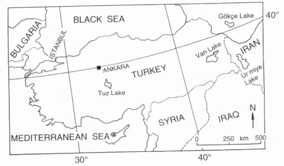
The world’s largest soda lake, Lake Van, located on the Anatolian high plateau in eastern Turkey (38.50N and 430E), (Fig. 1), experiences severe winters with frequent temperatures below 0oC. In winter, most precipitation falls as snow and, towards the end of spring, heavy rainfalls occur. High runoff rates in spring during snowmelt result in more than 80% of the annual discharge from the catchment reaching the lake during this period. The summer (July to September) is warm and dry, with average temperatures of 20oC. Diurnal temperature variations are about 20oC.
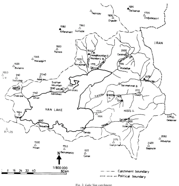
Lake Van has a drainage basin of 12 500 km2 (Fig. 2) and the lake surface presently averages about 3600 km2 (Kempe et al., 1978). The surface is approximately 1650 m above mean sea level. The lake is surrounded by hills and mountains which reach 4000 m above mean sea level. The volcanic mass, Süphan Mountain, rises to about 4434 m.
Lake Van has no natural outlets. It is the world’s fourth closed basin lake, with a volume of about 600 km3. From the lake surface, on average, 4.2 km3 of water is lost annually to the atmosphere by evaporation; this is balanced by the long-term averages of annual surface runoff and precipitation amounts of 2.5 km3 and 1.7 km3, respectively. Kadioglu et al. (1997) have shown that the fluctuations in water level are entirely dependent on the natural variability
Triple diagram model of level fluctuations in Lake Van, Turkey 237 0 50 100 150 200 250 300 350 400 450 0 100 200 300 400 500 Tim e, m o nths Le v e ls, cm
Fig. 2. Lake Van catchment.
of the hydrological cycle and on any longer term climatic changes which affect the drainage basin.
In the last decade, the water level in Lake Van has risen about 2 m; and, consequently, the low-lying inundated areas along the shore are now concerning local administrators and government officials, and affecting irrigation activities and people’s properties. Figure 3 shows monthly lake level fluctuations at a staff gauge located at the western corner of the lake from 1944–1994; each year, water level rises from January to June and falls thereafter. In this figure, the vertical axis indicates the readings from. These changes are
term lake level average is at 1648 m. Under prevailing climatic conditions, the lake level fluctuations have yearly amplitudes of 40–60 cm. Degens and Kurtman (1978) calculated the average annual amplitude as 49.7 ± 18 cm for the period 1944–1974. However, the record from 1944 to 1994 has average and standard deviation values of 136.8 cm and 70.8 cm, respectively (Sen et al., 1999). Comparison of these two periods shows increases of 275% and 383% in the mean lake level and amplitude, respectively, as a result of a rise in lake water level 1974, perhaps caused by a change in climate in the area. As a result the region has become more humid with more precipitation but less evaporation. In consequence, it is not realistic to assume linear, normal and stationary lake level fluctuations.
Triple diagram method (TDM)
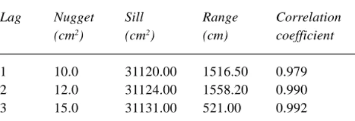
Human beings can visualise variations in three dimensions, using Cartesian coordinate systems through contour maps. Generally, maps are regarded as the variation of a variable by location variables that are either longitudes and latitudes or eastings and northings (Isaaks and Srivastava, 1989; Cressie, 1993; Kitanidis, 1997). Hence, it is possible to estimate the concerned (mapped) variable value for a given pair of location variables. Similarly, since one wants to predict the current lake level from previous records, it is suggested that two previous records replace the two location variables. Thus the current value of a variable can be mapped, based on two previous values of the same variable. The first step prior to mapping is to determine the empirical SV which guides the theoretical model that will be employed in the classical Kriging modelling. For this purpose, the scatter of SV values versus distance is obtained for lag-one, -two and -three. To depict the general trend of the scatter diagram, the distance range is divided into nine intervals, and the average of the SV values that fall at each interval is considered as the representative SV value within the mid-point distance of that interval as suggested by Myers et al. (1982). Different theoretical SV models such as linear, power, spherical and Gaussian types have been tried for the best fit and, in the end, the Gaussian SV was the best match to the experimental SV trend (Fig. 4). The Gaussian model is the most suitable in all lags and the properties of a fitted Gaussian SV model are presented in Table 1.
Such a mapping technique is referred to hereafter as triple diagram methodology (TDM). Such maps are based on three consecutive lake levels. TDMs help to make interpretations in spite of extremely scattered points. Although for mapping Davis (1986) has suggested the application of various simple regional techniques such as inverse distance, inverse distance square, etc. which consider the geometrical
configuration of the scatter points only without the use of a third variable. In this paper, preparation of the TDM is based on classical Kriging technique.
The construction of a TDM requires three variables, two of which are referred to as independent variables (predictors) and constitute the basic scatter diagram. The third is the dependent variable, which has its measured values attached to each scatter point. The equal value lines are constructed
Triple diagram model of level fluctuations in Lake Van, Turkey
239
by the Kriging methodology concept, which is also referred to as geostatistics (Matheron, 1963). Details of this methodology are explained for earth sciences applications by Journel and Huijbregts (1978), Isaaks and Srivastava (1989) and Cressie (1993).
The geostatistical methods take into consideration the effective role of the measured values of a regional variable at a set of irregular sites. In this paper, the positions of irregular sites constitute the scatter points of two independent variables. In the scatter diagram attached to its points are the values of the dependent variable, which is then mapped by conventional Kriging methodology. The resulting map appears in the form of contour lines covering the whole variability domains of the two independent variables. Preparation of such a map referring to the TDM triple diagram helps to predict the value of the mapped variable given the values of the independent variables. Detailed information concerning the mapping procedure by Kriging is presented elsewhere (Matheron, 1963; Journal and Huijbrets, 1977; Kitanidis, 1997).
Application and interpretations
Lake Van water level records are used with Kriging methodology to obtain triple diagrams that give the common behaviour of three variables, which are taken consequently from the historical time series data. The first two variables represent two past lake levels and the third indicates the present lake level. Hence, the model has three parts, namely, observations (recorded time series) as input, triple diagram as response and the output as prediction. Lags between the successive data at one, two, three, etc. intervals can be considered. Such an approach is very similar to a second-order Markov process, which can be expressed as
i 2 i 1 i i H H H =α − +β − +ε (1)
where Hi, Hi-1 and Hi-2 are the three consecutive lake levels; α and β are model parameters and εi is the error term. Prior to any prediction procedure, the application of such a model requires parameter estimations from the available data. Furthermore, its application requires assumptions which
include linearity, normality (Gaussian distribution of the residuals, i.e. εi’s), variance constancy, ergodicity and independence of residuals. The triple diagram in the form of a map replaces Eqn.(1) without any restriction. Such a map has the appearance of a natural relationship between three consecutive time values of the same variable.
To apply the triple diagram approach, the data must be divided into training and testing parts. Hence, 24 months (two years, 1984,1985) are used for the test (prediction) whereas all the other values are employed for training, which is the mapping. Maps are prepared according to a Kriging procedure through available software programs. Prior to any prediction, the following interpretations can be drawn from these figures.
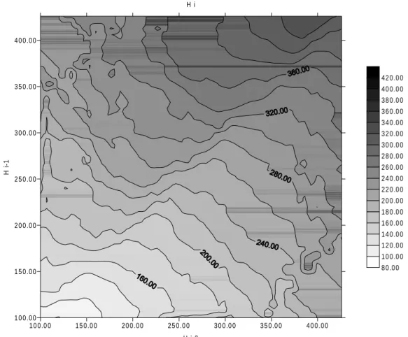
(1) In the case of lag-one there is a strong relationship between Hi-1 and Hi-2 with increasing contour values of Hi along the 45o line (see Fig. 5). The small H
i values are concentrated at small Hi-1 and Hi-2 values, this implies the clustering of small values of the three consecutive lake levels. Similarly, high lake level values of the three consecutive levels also constitute a high value cluster. That small values follow small values and high values follow high values indicates positive correlations. Local variations in the contour lines appear at either low (high) Hi-1 and high (low) Hi-2 values. Consequently, better predictions can be expected within a certain band around the 45o line. The following set of logical rules can be deduced from Fig. 6.
IF Hi-1 is low and Hi-2 is low THEN Hi is low, IF Hi-1 is medium low and Hi-2 is medium THEN Hi
is medium,
IF Hi-1 is high and Hi-2 is high THEN Hi is high, These rules can be used for a fuzzy logic inference system as suggested by Zadeh (1968).
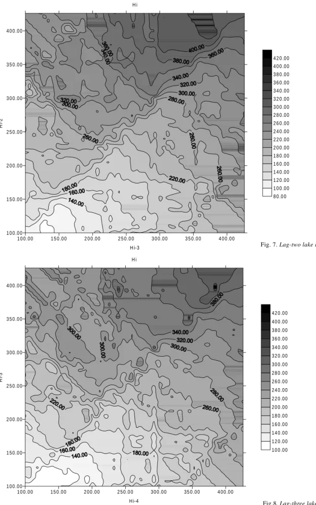
(2) In Fig. 7 (lag-two), the variations in the contour lines become very distinctive and rather haphazard compared with Fig. 5. This implies that with the increment in the lag value, present time lake level prediction will have more relative error. There is also a distinctive 45o line but with a comparatively narrower band of certainty around it.
(3) Finally, at lag-three case (Fig. 8) the contour pattern is even more haphazard. This implies an increase in the relative error of predictions.
Sen et al. (2000) identified suitable models and estimates for lake level fluctuations and their parameters for trend, periodic and stochastic parts. A second order Markov model is found suitable for the stochastic part. Triple diagrams of lake levels can replace the second order Markov process.
Table 1. Theoretical Gaussian semivariogram parameters Lag Nugget Sill Range Correlation
(cm2) (cm2) (cm) coefficient
1 10.0 31120.00 1516.50 0.979
2 12.0 31124.00 1558.20 0.990
10 0.0 0 15 0.0 0 20 0.00 25 0.0 0 30 0.0 0 35 0.0 0 40 0.00 H i-2 H i 10 0.00 15 0.00 20 0.00 25 0.00 30 0.00 35 0.00 40 0.00 H i -1 80 .00 10 0.0 0 12 0.0 0 14 0.0 0 16 0.0 0 18 0.0 0 20 0.0 0 22 0.0 0 24 0.0 0 26 0.0 0 28 0.0 0 30 0.0 0 32 0.0 0 34 0.0 0 36 0.0 0 38 0.0 0 40 0.0 0 42 0.0 0 80 130 180 230 280 330 380 430 80 180 280 380 Actu al Es t ima t e d
Fig. 5. Lag-one lake level triple diagram
Fig. 6. Lag-one cross-validation
In this manner, it is not necessary to use first and second order autocorrelation coefficients, in order to take more persistence into account. To make predictions for the 24 months that are not used in constructing the triple diagrams shown in Figs. 5, 7 and 8, Hi-k and Hi-k-1 for each month must be emtered on vertical and horizontal axes, respectively. The prediction value of Hi can either be read from this map approximately, or calculated using Kriging prediction equations, which is the course taken in this paper. The prediction results are shown in Table 2 with corresponding relative error amounts. Individual errors are
slightly greater than 10% but the overall prediction of relative error percentage is about 2.16%. Figure 9 indicates the observed and predicted Hi values which follow each other very closely; on average, observed and predicted lake level series have almost the same statistical parameters. The triple diagram model depicts even the increasing trend, which is not possible directly with the second order Markov process. During the prediction procedure, there is no special treatment for trend, but even so it is modelled successfully. However, in any stochastic or statistical modelling, it is first necessary to make a trend analysis and separate it from the original data. To verify the triple diagram approach for lake level predictions, in Fig. 9 the test data are plotted against the predictions; almost all the points are around the 45o line and hence the model is not biased. Predictions are successful at low or high values.
It is possible to look at the triple diagram model performance at two and three lag values. Figures 10 and 11 show that while the deviations of predictions are larger than those in Fig. 9, they still depict the general trend. The prediction results, shown in Tables 3 and 4 demonstrate numerically that increases in the lag cause increases in the relative error.
Triple diagram model of level fluctuations in Lake Van, Turkey 241 1 0 0.00 1 5 0 .00 2 0 0 .00 2 5 0 .0 0 3 0 0.00 3 5 0 .00 4 0 0 .00 H i-3 H i 1 0 0 .00 1 5 0 .00 2 0 0 .00 2 5 0 .00 3 0 0 .00 3 5 0 .00 4 0 0 .00 Hi -2 8 0 .0 0 1 0 0 .00 1 2 0 .00 1 4 0 .00 1 6 0 .00 1 8 0 .00 2 0 0 .00 2 2 0 .00 2 4 0 .00 2 6 0 .00 2 8 0 .00 3 0 0 .00 3 2 0 .00 3 4 0 .00 3 6 0 .00 3 8 0 .00 4 0 0 .00 4 2 0 .00 1 0 0 .0 0 1 5 0 .0 0 2 0 0 .0 0 2 5 0 .0 0 3 0 0 .0 0 3 5 0 .0 0 4 0 0 .0 0 H i-4 H i 1 0 0 .0 0 1 5 0 .0 0 2 0 0 .0 0 2 5 0 .0 0 3 0 0 .0 0 3 5 0 .0 0 4 0 0 .0 0 Hi -3 1 0 0 .0 0 1 2 0 .0 0 1 4 0 .0 0 1 6 0 .0 0 1 8 0 .0 0 2 0 0 .0 0 2 2 0 .0 0 2 4 0 .0 0 2 6 0 .0 0 2 8 0 .0 0 3 0 0 .0 0 3 2 0 .0 0 3 4 0 .0 0 3 6 0 .0 0 3 8 0 .0 0 4 0 0 .0 0 4 2 0 .0 0
Fig. 7. Lag-two lake level triple diagram
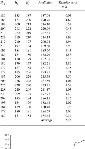
Table 2. Lag-one lake level prediction (cm)
Hi-2 Hi-1 Hi Prediction Relative error (%) 180 183 187 187.06 0.03 183 187 200 190.76 4.62 187 200 213 214.10 0.52 200 213 222 220.99 0.45 213 222 219 227.61 3.78 222 219 210 214.13 1.93 219 210 197 200.94 1.96 210 197 184 189.50 2.90 197 184 181 183.60 1.41 184 181 180 182.79 1.53 181 180 179 182.95 2.16 180 179 177 182.21 2.86 179 177 185 181.02 2.15 177 185 206 193.21 6.21 185 206 226 213.56 5.50 206 226 228 237.59 4.04 226 228 220 223.41 1.52 228 220 209 211.17 1.03 220 209 195 197.77 1.40 209 195 184 186.15 1.16 195 184 179 182.68 2.02 184 179 180 180.48 0.26 179 180 181 184.69 2.00 180 181 184 184.63 0.34 Average 2.16 0 50 100 150 200 250 300 350 400 450 0 5 10 15 20 25 30 Tim e (m o nth s) La k e l ev e l (c m ) observation prediction 0 50 100 150 200 250 300 350 400 450 0 5 10 15 20 25 30 Tim e (m o n th s) La k e l ev e l (c m ) observation prediction
Fig. 9. Observed and predicted lake levels at lag-one for the test
data
Conclusions
The concept of the triple diagram method (TDM) based on a single variable such as lake level is presented for tmaking predictions from past records. The diagram is a map with two independent values of the same variable at successive time intervals and the contours picture the current values of
Fig.10. Observed and predicted lake levels at lag-two for the test
data 0 50 100 150 200 250 300 350 400 450 0 5 10 15 20 25 30 Tim e (m o n th s) L a ke leve l (c m ) observation prediction
Fig. 11. Observed and predicted lake levels at lag-three for the test
data
the same variable. In any application, the TDM map is drawn using classical Kriging methodology based on the training data set, which includes the first portion of the available record. The TDM map is used for prediction provided that the values of two independent variables are given. The TDM may be regarded as the mapping form of a second order Markov process where three successive record values are related to each other. In the TDM, there no restrictive assumptions such as linearity, normality, stationarity, ergodicity, independence of residuals, etc. Besides, it does need estimations of first and second order autocorrelation coefficients for prediction and yields more accurate predictions. The methodology has been applied to water level fluctuation records in Lake Van, in eastern Turkey. The predictions are obtained for the two-year (24 months) test data at lags of one, two and three. In all three lags, the overall prediction relative error is less than 10%, which is acceptable in practical terms. In the case of the lag-one triple diagram prediction, the relative error is the least (less than 5%). The procedure presented in this table can be used to predict any hydrological variable.
Triple diagram model of level fluctuations in Lake Van, Turkey
243
Table 3. Lag-two lake level predictions (cm)
Hi-3 Hi-2 Hi Prediction Relative error (%) 181 180 187 184.88 1.13 180 183 200 191.20 4.40 183 187 213 196.44 7.78 187 200 222 219.85 0.97 200 213 219 237.44 7.77 213 222 210 221.62 5.24 222 219 197 207.85 5.22 219 210 184 195.08 5.68 210 197 181 188.63 4.04 197 184 180 182.73 1.50 184 181 179 185.51 3.51 181 180 177 184.88 4.26 180 179 185 184.07 0.51 179 177 206 184.78 10.30 177 185 226 200.15 11.44 185 206 228 211.61 7.19 206 226 220 238.44 7.74 226 228 209 217.65 3.98 228 220 195 200.21 2.60 220 209 184 191.04 3.69 209 195 179 184.24 2.85 195 184 180 181.43 0.79 184 179 181 182.28 0.70 179 180 184 188.00 2.13 Average 4.39
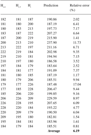
Table 4. Lag-three lake level predictions (cm)
Hi-4 Hi-3 Hi Prediction Relative error (%) 182 181 187 190.86 2.02 181 180 200 187.19 6.41 180 183 213 197.73 7.17 183 187 222 207.27 6.64 187 200 219 215.90 1.41 200 213 210 237.90 11.73 213 222 197 211.16 6.71 222 219 184 202.98 9.35 219 210 181 194.94 7.15 210 197 180 186.58 3.52 197 184 179 183.64 2.52 184 181 177 191.09 7.37 181 180 185 187.19 1.17 180 179 206 185.51 9.94 179 177 226 187.48 17.04 177 185 228 206.47 9.44 185 206 220 199.85 9.16 206 226 209 229.59 8.97 226 228 195 207.65 6.09 228 220 184 193.22 4.77 220 209 179 190.50 6.04 209 195 180 182.81 1.54 195 184 181 183.96 1.61 184 179 184 185.51 0.81 Average 6.19
References
Box, G.F.P. and Jenkins, G.M., 1976. Time series analysis
forecasting and control. Holden Day, San Francisco, USA. 560
pp.
Cressie, N.A.C., 1993. Statistics for spatial data, revised edition. Wiley, New York, USA. 900pp.
Davis, J.C., 1986. Statistics and data analysis in geology. Wiley, New York, USA. 646pp.
Degens, E.T. and Kurtman, F., 1978. The geology of Lake Van. Rept. 169, The Mineral Research and Exploration Institute of Turkey. 158 pp.
Hubert, P., Carbomnel, J.D. and Chaouche, A., 1989. Segmentation des series hydrometeoraloques: application a des series de precipitation et de debits de L’Afrique de L’ouest. J. Hydrol., 110, 349–367
Iruine, K.N. and Eberthardt, A.K.,1992. Multiplicative seasonal ARIMA models for lake Erie and Lake Ontario water levels,
Water Resour. Bull., 28, 385–396.
Isaaks, E.H. and Srivastava, R.M., 1989. An Introduction to
Applied Geostatistics. Oxford Univ. Press, Oxford, 561 p.
Journel, A., and Huijbregts, A., 1978. Mining Geostatistics. Academic Press, London, UK.
Kadioglu, M., Sen, Z. and Batur, F., 1997. The greatest soda-water lake in the world and how it is influenced by climatic change.
Ann. Geophysicae, 15, 1489–1497.
Kempe, S., Khoo, F. and Gürleyik, V., 1978. Hydrography of lake Van and its drainage area. In: Geology of Lake Van, E.T. Degen and F. Kurtman, (Eds.), The Mineral Research and Exploration Institute of Turkey, Rep. 169, 30–45.
Kite, V., 1990. Time series analysis of Lake Erie levels. In: Proc
Symp. Great Lakes Water Level Forecasting and Statistics, H.C.
Hurtmann and M.J. Donalhue (Eds.), Great Lake Comission, Ann Arbor, Michigan, USA. 265–277.
Loucks, F.D., 1989. Modeling the Great Lakes
hydrologic-hydraulic system. PhD Thesis, University of Wisconsin,
Madison, USA.
Matheron, G., 1963. Principles of geostatistics. Econ. Geol., 58,1246–1266.
Mathier, L., Fagherazzi, L., Rasson, J.C. and Bobee, B., 1992. Great Lakes net basin supply simulation by a stochastic approach. INRS-Eau Rapp Scientifique 362, INRS-Fau, Sainte-Foy. 95 pp.
Myers, D.E., Begovich, C.L., Butz, T.R. and Kane, V.E., 1982. Variogram models for regional groundwater chemical data.
Math. Geol., 14, 629–644.
Privalsky, V., 1990. Statistical analysis and predictability of Lake Erie water level variations. In: Proc Symp. Great Lakes Water
Level Forecasting and Statistics, H.C. Hurtmann and M.J.
Donalhue (Eds.), Great Lake Comission, Ann Arbor, Michigan, USA. 255–264.
Sen, Z., Kadýoðlu, M. and Batur, E., 1999. Cluster regression model and level fluctuation features of Van Lake, Turkey. Ann.
Geophysicae, 17, 273–279.
Sen. Z., Kadioglu, M. and Batur, E., 2000. Stochastic modeling of the Van Lake monthly fluctuations in Turkey. Theor. Appl.
Climatol., 65, 99–110.
Slivitzky, M. and Mathier, L., 1993. Climatic changes during the 20th century on the Laurentian Great Lakes and their impacts on hydrologic regime. NATO Adv. Study Inst., Deauaille, France. Sneyers, R., 1992. On the use of statistical analysis for the objective
determination of climate change. Meteorol. Z., 1, 247–256. Vannitseni, S. and Demaree, G., 1991. Detection et modelisation
des secheresses an Sahel-proposition d’une nouvelle methodologie. Hydra Continent, 6, 155–17.
Zadeh, L.A., 1968. Fuzzy algorithms. Information and Control, 12, 94–102.