HAL Id: hal-00169438
https://hal.archives-ouvertes.fr/hal-00169438
Submitted on 4 Sep 2007
HAL is a multi-disciplinary open access
archive for the deposit and dissemination of
sci-entific research documents, whether they are
pub-lished or not. The documents may come from
teaching and research institutions in France or
abroad, or from public or private research centers.
L’archive ouverte pluridisciplinaire HAL, est
destinée au dépôt et à la diffusion de documents
scientifiques de niveau recherche, publiés ou non,
émanant des établissements d’enseignement et de
recherche français ou étrangers, des laboratoires
publics ou privés.
Observation of enhanced X-ray emission from the CTTS
AA Tau during a transit of an accretion funnel
Nicolas Grosso, Jérôme Bouvier, Thierry Montmerle, Matilde Fernández,
Konstantin Grankin, Maria Rosa Zapatero Osorio
To cite this version:
Nicolas Grosso, Jérôme Bouvier, Thierry Montmerle, Matilde Fernández, Konstantin Grankin, et al..
Observation of enhanced X-ray emission from the CTTS AA Tau during a transit of an accretion
funnel. Astronomy and Astrophysics - A&A, EDP Sciences, 2007, 475 (2), pp.607-617. �hal-00169438�
hal-00169438, version 1 - 4 Sep 2007
September 4, 2007
Observation of enhanced X-ray emission from the CTTS AA Tau
during a transit of an accretion funnel flow
⋆
N. Grosso
1, J. Bouvier
2, T. Montmerle
2, M. Fern´andez
3, K. Grankin
4, and M.R. Zapatero Osorio
51 Observatoire astronomique de Strasbourg, Universit´e Louis-Pasteur, CNRS, INSU, 11 rue de l’Universit´e, 67000 Strasbourg, France 2 Laboratoire d’astrophysique de Grenoble, Universit´e Joseph-Fourier, CNRS, INSU, 414 rue de la Piscine, 38041 Grenoble, France 3 Instituto de Astrof´ısica de Andaluc´ıa, CSIC, Camino Bajo de Hu´etor 50, 18008 Granada, Spain
4 Ulugh Beg Astronomical Institute of the Uzbek Academy of Sciences, Astronomicheskaya 33, 700052 Tashkent, Uzbekistan 5 Instituto de Astrof´ısica de Canarias (IAC), v´ıa L´actea s/n, 38205 La Laguna, Tenerife, Spain
Received 15 June 2007 / Accepted 27 August 2007
ABSTRACT
Context.Classical T Tauri stars are young solar-type stars accreting material from their circumstellar disks. Thanks to a favorable inclination of the system, the classical T Tauri star AA Tau exhibits periodic optical eclipses as the warped inner disk edge occults the stellar photosphere.
Aims.We intend to observe the X-ray and UV emission of AA Tau during the optical eclipses with the aim to localize these emitting regions on the star.
Methods.AA Tau was observed for about 5 h perXMM-Newton orbit (2 days) over 8 successive orbits, which covers two optical eclipse periods (8.22 days). TheXMM-Newton optical/UV monitor simultaneously provided UV photometry (UVW2 filter at 206 nm) with a ∼15 min sampling rate. Some V-band photometry was also obtained from the ground during this period in order to determine the dates of the eclipses.
Results.Two X-ray and UV measurements were secured close to the center of the eclipse (∆V ∼ 1.5 mag). The UV flux is the highest just before the eclipse starts and the lowest towards the end of it. UV flux variations amount to a few 0.1 mag on a few hours timescale, and up to 1 mag on a week timescale, none of which are correlated with the X-ray flux. We model it with a weekly modulation (inner disk eclipse), plus a daily modulation, which suggests a non-steady accretion, but needs a longer observation to be confirmed. No such eclipses are detected in X-rays. Within each 5 h-long observations, AA Tau has a nearly constant X-ray count rate. On a timescale of days to weeks, the X-ray flux varies by a factor of 2–8, except for one measurement where the X-ray count rate was nearly 50 times stronger than the minimum observed level even though photoelectric absorption was the highest at this phase, and the plasma temperature reached 60 MK, i.e. a factor of 2–3 higher than in the other observations. This X-ray event, observed close to the center of the optical eclipse, is interpreted as an X-ray flare.
Conclusions. We identify the variable column density with the low-density accretion funnel flows blanketing the magnetosphere. The lack of X-ray eclipses indicates that X-ray emitting regions are located at high latitudes. Furthermore, the occurrence of a strong X-ray flare near the center of the optical eclipse suggests that the magnetically active areas are closely associated with the base of the high-density accretion funnel flow. We speculate that the impact of this free falling accretion flow onto the strong magnetic field of the stellar corona may boost the X-ray emission.
Key words.Stars: individual: AA Tau – Stars: pre-main sequence – Stars: flare – X-rays: stars – Accretion, accretion disks
1. Introduction
T Tauri stars (TTSs), i.e. young (1–10 Myrs) solar-type stars, are conspicuous X-ray emitters. Their high X-ray luminosities (LX ≃ 1028−31erg s−1) compared to the Sun (LX ≃ 1027erg s−1 at solar maximum), and intense flaring activity (up to LX ≃ 1032−33erg s−1) make them appear as extremelly active young Suns in the X-ray domain. The analogy with the solar activ-ity has been quite successful in ascribing the X-ray emission of TTSs to an optically thin, magnetically confined coronal plasma in collisional equilibrium at temperatures of 10–100 MK, emit-ting a thermal bremsstrahlung continuum and emission lines (see, e.g., review by Feigelson & Montmerle 1999). As ob-served in the X-ray coronae of active stars (e.g., Ness et al. 2004), the enhanced X-ray luminosity of TTSs can easily be ex-plained by coronal structures with high plasma density, because
⋆ Figures 2, 3 and 9, and Appendix A are only available in electronic
form via http://www.edpsciences.org .
the X-ray luminosity is proportional to the plasma emission mea-sure, which scales linearly with the plasma volume but with the square of the plasma electronic density. That most of TTSs X-ray emission arises in an active magnetic corona is supported by direct Zeeman measurements on photospheric spectral lines which indicate surface magnetic fields of a few kilogauss (e.g., Guenther et al. 1999; Johns-Krull et al. 1999, 2004; Johns-Krull 2007; Yang et al. 2005). However, the dynamo mechanism pro-ducing the magnetic field in these fully convective stars is still discussed (e.g., Preibisch et al. 2005; Briggs et al. 2007).
The solar paradigm, where the X-ray emitting plasma is con-fined in magnetic loop with both feet anchored on the stellar pho-tosphere, has been questionned in the context of a Classical TTS (CTTS), which accretes material from its circumstellar disk. Inside a few stellar radii above the CTTS surface, the stellar magnetic field pressure is larger than the ram pressure of the ac-creting gas. As a result, the stellar magnetosphere truncates the inner accretion disk and controls the accretion flows. The gas is
mainly accreted from the disk edge to the stellar surface along the dominant large scale stellar magnetic lines, creating accre-tion funnel flows. The free-falling gas hits the stellar surface at the feet of the accretion funnel flows, where the kinetic energy is dissipated in a shock producing hot excess emission (see review on magnetospheric accretion by Bouvier et al. 2007b).
The X-ray grating spectrometers aboardChandraand XMM-Newtonare able to obtain spectra of the X-ray brightest CTTSs, where the emission line triplets of He-like elements are re-solved, which provides a powerful tool to assess the elec-tronic density of the X-ray emitting plasma (e.g., Porquet et al. 2001). In several CTTSs, plasma with high electronic density (ne ∼ 1013cm−2) and low temperature (∼3 MK), untypical of stellar coronae, were identified, and therefore attributed to accretion shocks (Kastner et al. 2002; Stelzer & Schmitt 2004; Schmitt et al. 2005; Robrade & Schmitt 2006; Argiroffi et al. 2007; G¨unther et al. 2007; Telleschi et al. 2007); whereas some CTTSs display no such evidence (Audard et al. 2005; Smith et al. 2005; G¨udel et al. 2007b).
During the Chandra Orion Ultradeep Project (COUP, see Getman et al. 2005b), where the TTSs of the Orion nebula clus-ter were monitored nearly continuously over ∼13 days with the Advanced CCD Imaging Spectrometer, numerous X-ray flares were observed. In a few cases, a size of several stellar radii was derived for the magnetic loop confining the X-ray emitting plasma, large enough to connect the stellar surface with the edge of the accretion disk (Favata et al. 2005).
We propose to directly constrain the source and location of the X-ray emission in CTTSs by using eclipses. Eclipse map-ping have been successfully used in binary active stars to recon-struct the coronae (e.g., G¨udel et al. 2001, 2003), or to localize the flaring plasma (e.g., Schmitt & Favata 1999; Schmitt et al. 2003). Our target star is AA Tau, located in the Taurus molec-ular cloud complex at a distance of ∼140 pc (e.g., Kenyon et al. 1994). AA Tau is a quite typical member of the CTTS class, with a K7 spectral type, a bolometric luminosity of ∼0.8 L⊙, a stel-lar mass of ∼0.8 M⊙, and a stellar radius of ∼1.85 R⊙; exhibit-ing moderate accretion disk diagnostics (near-IR excess, optical veiling, Balmer line emission), but with the remarkable prop-erty to be viewed nearly edge-on. Bouvier et al. (1999, 2003, 2007a) reported evidence for a modulation of the photospheric flux and spectroscopic diagnostics with a period of 8.22 days, corresponding to the rotational period of the star. This stellar flux modulation was interpreted as the periodic eclipse of the stellar photosphere by the optically thick, magnetically-warp in-ner disk edge located at 8.8 stellar radii. Photopolarimetric vari-ations confirm the presence of an optically thick wall located at the disk edge, and eclipsing periodically the stellar photosphere (M´enard et al. 2003).
We obtained 8 observations of AA Tau with XMM-Newton(Jansen et al. 2001), which allows simultaneous obser-vations with an EPIC pn (Str¨uder et al. 2001) and two EPIC MOS (Turner et al. 2001) X-ray spectroimaging cameras, and the Optical/UV monitor (OM; Mason et al. 2001). We sup-plemented these X-rays and UV observations with an optical ground-based monitoring of AA Tau to secure the dates of the optical eclipses. TheseXMM-Newtonobservations were previ-ously reported in Schmitt & Robrade (2007, hereafter SR), who used the minimum of the UV light curve as proxy of the optical eclipse. SR found variable X-ray absorption “such that the times of maximal X-ray absorption and UV extinction coincide”. SR introduced an additional absorption in a disk wind, or a peculiar dust grain distribution to reconcile the high value of the X-ray absorption outside the eclipse and the low optical extinction.
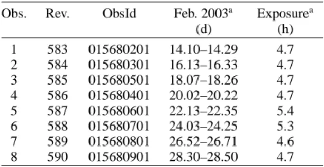
Table 1. Journal of the XMM-Newton observations of AA Tau (PI: J. Bouvier).
Obs. Rev. ObsId Feb. 2003a Exposurea
(d) (h) 1 583 015680201 14.10–14.29 4.7 2 584 015680301 16.13–16.33 4.7 3 585 015680501 18.07–18.26 4.7 4 586 015680401 20.02–20.22 4.7 5 587 015680601 22.13–22.35 5.4 6 588 015680701 24.03–24.25 5.3 7 589 015680801 26.52–26.71 4.6 8 590 015680901 28.30–28.50 4.7
a The observation beginning, end, and duration is given for MOS1.
In Sect. 2, we present the X-ray and UV properties of AA Tau based on a reanalysing of the full data set provided by theseXMM-Newtonobservations. In particular, we report X-ray (pn+MOS1+MOS2) and UV light curves with a time resolution of ∼15 min. We show that a bright and hot flare was observed during the second observation. In Sect. 3, thanks to our ground-based observations and optical OM data, we determine the dates of the optical eclipses, which allow us to compare the UV and X-ray variabilities versus the rotational phase. We show that the UV minimum is outside the eclipse, and that the (confirmed) varia-tion of the column density are not correlated with the rotavaria-tional phase. In Sect. 4, we propose another origin for this variable col-umn density, and we discuss the origin of the X-ray flare that was observed during an optical eclipse.
2. X-ray and UV properties of AA Tau
2.1. XMM-Newton observations and event selections
Our observational strategy withXMM-Newtonwas to cover two consecutive modulation periods (∼17 days) in order to demon-strate the reproducibility of the phenomenon from one rotational cycle to the next. The temporal sampling of the X-ray light curve needs not to be very dense because AA Tau spends nearly the same amount of time being eclipsed as being entirely vis-ible. Therefore, we requested one 4 h-exposure with EPIC pn per XMM-Newtonorbit (2 days) over 8 successive orbits. We used the full frame science mode of the EPIC cameras with the medium optical blocking filter. The pointing nominal co-ordinates were 04h34m55.s5, 24◦28′54.′′0 (J2000 equinox). The journal of theXMM-Newtonobservations of AA Tau is given in Table 1.
The data reduction was made using the XMM-Newton Science Analysing System (SAS, version 7.0.0) For each observations, the event lists for each camera of EPIC were produced using the SAS tasks epchain and emchain, respectively. We used the background lightcurves computed by these task in the 7.0–15.0 keV energy range to determine the time intervals affected by background proton flares. More than half of the observing time is affected by bad space weather. For each instrument, we made from the low background time intervals a sky image with 3′′-pixels in the 0.5–7.3 keV energy range1. The X-ray counterpart of AA Tau was detected in all the observations.
1 We selected single, double, triple, and quadruple pixel events (i.e. PATTERN in the 0 to 12 range), and also applied the predefined filter
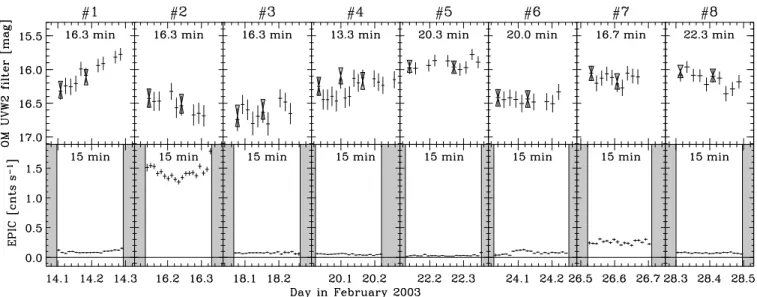
Fig. 1.XMM-Newtonobservations of AA Tau. Top and bottom panels show the background subtracted UV (180–250 nm) and X-ray (0.5–7.3 keV) light curves obtained with the Optical/UV Monitor (OM) and EPIC (pn+MOS1+MOS2), respectively. In each panel, the label indicates the time interval used to bin the light curve. Grey hourglasses and crosses data points indicate UV photometry obtained with the large and small OM central imaging window. The X-ray count rates are corrected from (circular) aperture. The gray stripes indicate the beginning and the end of the EPIC observation.
For the X-ray light curves of AA Tau, we selected the source+background events within a circular region centered on AA Tau . The extraction position and radius were optimized to maximize the signal-to-noise ratio in the sky image. The back-ground in MOS and pn was extracted using an annular region centered on AA Tau and a box region at the same distance to the CCD readout node, respectively, where areas illuminated by other weak X-ray sources were excluded. For the X-ray spec-tra, we used the same extraction regions and only time inter-vals with low background; we selected events with energy above 0.3 keV and the usual stronger selection criteria2. We computed the corresponding redistribution matrix files and ancillary re-sponse files.
2.2. X-ray light curves
For each instrument and observations, we first built the source+background and the background light curves with 1 s time bins starting at the first good time interval (GTI) of MOS1. We rebinned the light curve to 900 s to increase the signal. Then, we subtracted from the source+background light curve the back-ground light curve scaled to the same source extraction area.
From the GTI extension, we scaled up with an IDL routine count rates and errors affected by any lost of observing time, mainly due to the triggering of counting mode during high flar-ing background periods, when the count rate exceeded the de-tector telemetry limit. We also corrected count rates and errors for circular aperture photometry using the fraction of PSF counts inside the (circular) extraction region calculated by the SAS as-suming a fixed photon energy of 1.5 keV. Finally, the light curves of the three detectors were summed to produce the EPIC light curves. We estimated the missing pn data at the beginning of the observations by multiplying the MOS1+MOS2 count rates by
2 For pn, we selected only single and double pixel events (i.e. PATTERNin the 0 to 4 range) with FLAG value equal to zero; for MOS, we selected PATTERN in the 0 to 12 range, and applied the predefined filter #XMMEA SM.
1.17, the median scaling factor between MOS1+MOS and pn in the second observation where AA Tau was the brightest.
The bottom panel of Fig. 1 shows the EPIC light curves of AA Tau in the 0.5–7.3 keV energy range. Within each 5 h-long observations, AA Tau exhibited a nearly constant X-ray flux. The minimum X-ray flux, that we will call hereafter the qui-escent level, was observed during the observation #5, where the averaged EPIC count rate was 0.030 ± 0.002 counts s−1. On a timescale of days to weeks, the X-ray flux varies by a factor of 2–8, except between the end of the first observation and the beginning of the second observation, where the EPIC count rate jumped in less than 2 days from 0.093 ± 0.003 to 1.42 ± 0.01 counts s−1, i.e. a level 47 ± 3 times stronger than the quiescent level. Then, the EPIC count rate decayed in less than 2 days to 0.075 ± 0.003 counts s−1, i.e. a level only 2.5 ± 0.2 times stronger than the quiescent level.
Such large amplitudes in the X-ray fluxes of young stellar objects are usually observed during X-ray flares, which have typical light curves with fast rise and peak phase, and slower (exponential) decay phase, associated with fast heating and slow cooling of the magnetically confined plasma (e.g., Imanishi et al. 2003; Favata et al. 2005). X-ray flares with unusually long rise phases have also been reported (e.g., Grosso et al. 2004; Wang et al. 2007; Broos et al. 2007).
For a comparison purpose, we note that, assuming a typical convertion ratio between XMM-Newton/EPIC and Chandra/ACIS-I count rates (e.g., Ozawa et al. 2005), the aver-age EPIC count rate of AA Tau, ∼0.08 counts s−1at the distance of the Taurus molecular cloud (d ∼ 140 pc), would convert to ∼0.001 Chandra/ACIS-I counts s−1at the distance of the Orion nebula (d ∼ 450 pc). AA Tau, put in the Orion nebula cluster, would have then been brighter than 67% of the X-ray sources in the COUP. To check whether the behaviour of the light curve of AA Tau is consistent with the one of an X-ray flare, we can compare it to the light curve data set obtained in the COUP.
We use the COUP results of the Bayesian block (BB) vari-ability analysis (developed by Scargle 1998; adapted for the COUP data set and coded in IDL by one of us, N.G.), which segmented the X-ray light curves into a contiguous sequences
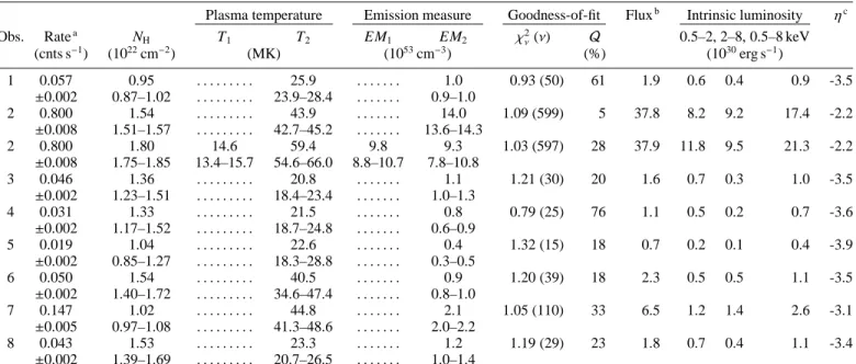
Table 2. Best parameters of simultaneous fitting of EPIC pn, MOS1, MOS2 spectra with XSPEC.
Plasma temperature Emission measure Goodness-of-fit Fluxb Intrinsic luminosity ηc
Obs. Ratea N H T1 T2 EM1 EM2 χ2ν(ν) Q 0.5–2, 2–8, 0.5–8 keV (cnts s−1) (1022cm−2) (MK) (1053cm−3) (%) (1030erg s−1) 1 0.057 0.95 . . . 25.9 . . . 1.0 0.93 (50) 61 1.9 0.6 0.4 0.9 -3.5 ±0.002 0.87–1.02 . . . 23.9–28.4 . . . 0.9–1.0 2 0.800 1.54 . . . 43.9 . . . 14.0 1.09 (599) 5 37.8 8.2 9.2 17.4 -2.2 ±0.008 1.51–1.57 . . . 42.7–45.2 . . . 13.6–14.3 2 0.800 1.80 14.6 59.4 9.8 9.3 1.03 (597) 28 37.9 11.8 9.5 21.3 -2.2 ±0.008 1.75–1.85 13.4–15.7 54.6–66.0 8.8–10.7 7.8–10.8 3 0.046 1.36 . . . 20.8 . . . 1.1 1.21 (30) 20 1.6 0.7 0.3 1.0 -3.5 ±0.002 1.23–1.51 . . . 18.4–23.4 . . . 1.0–1.3 4 0.031 1.33 . . . 21.5 . . . 0.8 0.79 (25) 76 1.1 0.5 0.2 0.7 -3.6 ±0.002 1.17–1.52 . . . 18.7–24.8 . . . 0.6–0.9 5 0.019 1.04 . . . 22.6 . . . 0.4 1.32 (15) 18 0.7 0.2 0.1 0.4 -3.9 ±0.002 0.85–1.27 . . . 18.3–28.8 . . . 0.3–0.5 6 0.050 1.54 . . . 40.5 . . . 0.9 1.20 (39) 18 2.3 0.5 0.5 1.1 -3.5 ±0.002 1.40–1.72 . . . 34.6–47.4 . . . 0.8–1.0 7 0.147 1.02 . . . 44.8 . . . 2.1 1.05 (110) 33 6.5 1.2 1.4 2.6 -3.1 ±0.005 0.97–1.08 . . . 41.3–48.6 . . . 2.0–2.2 8 0.043 1.53 . . . 23.3 . . . 1.2 1.19 (29) 23 1.8 0.7 0.4 1.1 -3.4 ±0.002 1.39–1.69 . . . 20.7–26.5 . . . 1.0–1.4
Notes: We fit the X-ray spectra with the continuum and emission lines produced by an optically thin plasma in thermal collisional ionization equilibrium model (vapec). We use for the plasma element abundances typical values observed in the coronae of young stars with fine X-ray spectroscopy (G¨udel et al. 2007a, see Table A.1). The wabs photoelectric absorption model use photoionization cross sections of Morrison & McCammon (1983), and solar abundances of Anders & Grevesse (1989). Errors are given at the 68% confidence level (i.e. ∆χ2= 1.0
for each parameter of interest), that corresponds to 1σ for Gaussian statistics. For observation #2, a better fit is obtained using a plasma with two temperature components.
a pn count rate (0.2–12 keV).
b Observed X-ray flux (0.5–8.0 keV) in unit of 10−13erg cm−2s−1.
c Logarithm of the X-ray intrinsic luminosity (0.5–8 keV) to the bolometric luminosity (0.8 L
⊙) ratio.
of constant count rates (see Getman et al. 2005b). We define a source to be variable, if there is more than one BB; with
BBmin and BBmax, the minimum and the maximum count rate levels, respectively (see, e.g., Stassun et al. 2007, for an appli-cation of COUP time-averaged X-ray variability). The latter and the former are viewed as the quiescent level and the peak level of the brightest flare, respectively. Applying this criteria, there are 977 variable sources (out of 1616 COUP sources). We find only 20 variable sources with peak amplitude (BBmax/BBmin) and duration larger than 45 and 4.7 h., respectively, as ob-served for AA Tau. For comparison, our subsample sources have
BBmax = 10−4–2 counts s−1, i.e., they are at peak between 200 times fainter and 100 times brighter than AA Tau (at the distance of the Orion nebula) at peak.
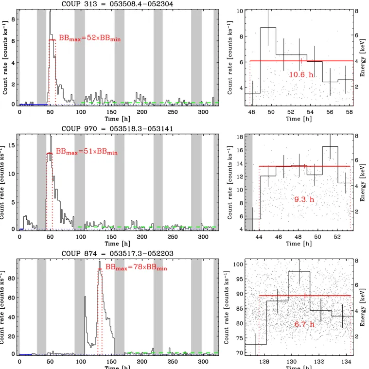
Then, we make a visual examination of the selected BB light curves to eliminate sources with peak flare BB having a spuri-ous long duration (including for example a passage through the van Allen belts), and/or sources with a decay phase too slow to reproduce the level observed at the beginning of the third ob-servation of AA Tau. For an exponential decay phase with a de-cay timescale τd, this latter criteria is equivalent to τd<0.6 day. Finally, we exhibit the brightest flares from COUP 313, 874, and 970, which fullfill our criteria (see online Fig. 2). These sources are bona fine members of the Orion nebula cluster (Getman et al. 2005a).
We conclude that a bright X-ray flare with a rapid cooling phase can well reproduce the large amplitude, and also the flat-ness of the light curve of AA Tau at its maximum. The following X-ray spectra analysis confirms this interpretation.
2.3. X-ray spectra and plasma parameters
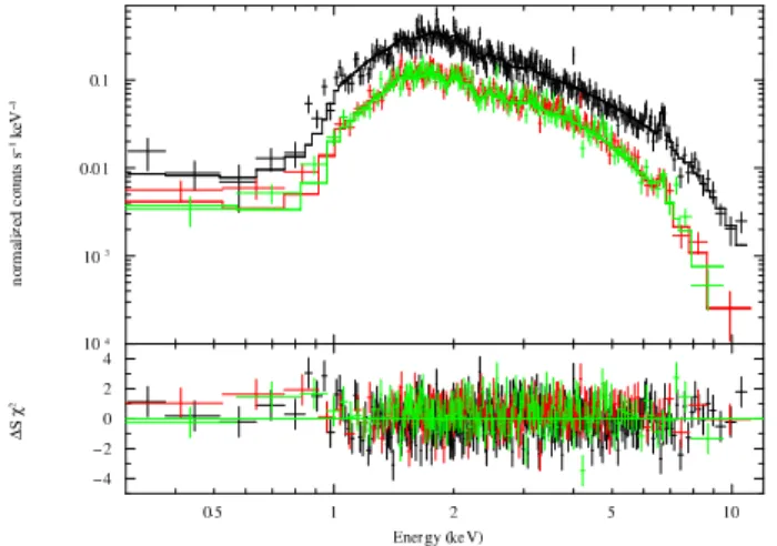
For each observations the pn, MOS1, and MOS2 spectra were binned to 25 counts per spectral bin. X-rays are detected up to 10 keV (see online Fig. 3). The spectra are featureless, except in the second observation where a prominent line around 6.7 keV is visible both in the pn and MOS spectra, corresponding to the FeXXVtriplet emission line (Fig. 4).
The pn, MOS1, and MOS2 spectra were fitted simultane-ously with XSPEC (version 12.3.0; Dorman & Arnaud 2001) to derive the plasma parameters. The model is an X-ray emission spectrum from collisionally-ionized diffuse gas, output from the Astrophysical Plasma Emission Code (vapec3), that in-cludes continuum and emission lines. The plasma element abun-dances were fixed to typical values measured in the coronae of young stars with grating X-ray spectroscopy (see online ap-pendix Table A.1), to allow a direct comparison with the XMM-Newton Extended Survey of the Taurus molecular cloud(XEST; G¨udel et al. 2007a). This emission model is combined with the wabsphotoelectric absorption model, which is based on the pho-toionization cross sections of Morrison & McCammon (1983), and the solar abundances of Anders & Grevesse (1989). The on-line Fig. 3 shows our best fits. For the second observation, we find a better fit by adding a second temperature component, which reduced the χ2from 655.4 (for 599 degrees of freedom; d.o.f.) to 617.2 (for 597 d.o.f.). Given the new and old values of χ2and number of degrees of freedom, a F-test indicates a prob-ability of ∼10−8for the null hypothesis; therefore, we conclude 3 More information can be found at:
Fig. 4. EPIC pn (black), MOS1 (red), MOS2 (green) spectra of
AA Tau for observation #2. The lines show our best fit using two temperature plasma combined with photoelectric absorption (Table 2). The residuals are plotted in sigma units with error bars of size one.
that it is reasonnable to add this extra temperature component to improve the fit. Our best fit with a two-temperature plasma is shown in Fig. 4.
Table 2 gives the corresponding plasma parameters.On timescale of 2-days, the photoelectric absorption of the X-ray spectra is not constant, but the observed relative variations are lower than a factor of two. The minimum and maximum values of the corresponding column density are ∼1.0 × 1022cm−2and 1.8 × 1022cm−2, respectively; the latter was observed during the second observation4. SR didn’t specify the model of X-ray ab-sorption that they used, but their one-temperature plasma model gave qualitatively similar results. We stress that the value of the column density can even be increased by 50% when revised so-lar abundances (i.e., metal poor) are adopted for the abundances of the absorbing material (see online Appendix A).
The plasma temperature is ∼23 MK during the low activ-ity levels. The observations showing an increase of X-ray count rates (namely #2, #6, and #7) also correspond to phases with the highest plasma temperatures (60 MK, 40 MK, and 45 MK, respectively), and therefore to flaring activity.
During the second observation the X-ray surface flux, i.e., the intrinsic X-ray luminosity divided by the stellar surface, peaked to 108erg s−1cm−2. The temperatures of the hot (60 MK) and cool (15 MK) plasma components, associated with this ele-vated level of X-ray surface flux, are consistent with the ones observed in the most active TTSs of COUP (see Fig. 11 of Preibisch et al. 2005). The cool plasma component is usually observed in the coronae of active stars, and may define a fun-damental coronal structure, which is probably related to a class of compact loops with high plasma density (see Preibisch et al. 2005, and references therein).
We make an estimate of the hot loop length using the method of Reale et al. (1997) (see also Favata et al. 2005, for an appli-cation on COUP data). Assuming a peak temperature of 60 MK and a flare decay time lower than 0.6 day (see Sect. 2.2), we find for the semi-circular loop a half-length lower than 7.1 R⋆ for a freely decaying loop, with no heating; or lower than 1.6 R⋆for
4 The increase of the spectrum slope between 1 and 2 keV observed
between observations #1 and #2, is not only due to the increase of the absorption, as argued in SR, but also for 20% to the increase of the plasma temperature.
a strongly sustained heating5 in the cooling phase. Therefore, the height of the semi-circular loop is lower than 1–4.5 R⋆. Therefore, this loop cannot connect the stellar surface and the inner accretion disk, distant by 7.8 stellar radii, and is likely an-chored on the stellar photosphere.
The high temperature and X-ray surface flux observed dur-ing the second observation point to an enhanced X-ray activity produced by a bright X-ray flare. Such bright flares on the Sun are sometimes associated with coronal mass ejection (CME). Therefore, we cannot rule out that the maximum of column den-sity observed during the second observation is due to this ener-getic event.
2.4. Comparison with previous X-ray observations of AA Tau AA Tau was previously observed several times in X-rays at dif-ferent epochs: on March 4, 1980 and February 7, 1981 with the IPC on boardEinstein, with an exposure of 0.6 h and 2.8 h, respectively; on August 10, 1990 during the ROSAT All Sky Survey(RASS) with the PSPC on boardROSAT, with an expo-sure of 0.2 h; and on February 22 and August 18, 1993 during two pointed PSPC observations of the young binary Haro 6-13 (PI: H. Zinnecker), with an exposure of 0.6 h and 1.5 h, respec-tively.
Walter & Kuhi (1981) reported a detection with 0.030 ± 0.005 IPC counts s−1, during the first observation with Einstein (bright enough to exhibit a crude spectrum), but only an upper limit of 0.004 IPC counts s−1 with a 5 times longer observation, nearly one year later (Walter & Kuhi 1984). Walter & Kuhi (1984) associated the X-ray emission detected from AA Tau as a quiescent level, and interpreted the non-detection in the framework of the smothered coronae of TTSs (see Walter & Kuhi 1981), where it was proposed that mass ejection could increase enough the absorbing column density to smother the coronal (quiescent) X-ray emission. Neuh¨auser et al. (1995) reported 10 years later a RASS de-tection with 0.014 ± 0.006 PSPC counts s−1.6 AA Tau was also detected during the PSPC pointed observation with 0.022 ± 0.005 PSPC counts s−1(see in the WGA catalogue of ROSAT point sources, the source 1WGA J0434.9+2428, located 37′ off-axis; White et al. 1996), but (again) only during the shortest ex-posure.
Further constraint can be derived on the X-ray variability of AA Tau by combining these multiple epoch observations with our better assessment of its quiescent level thanks to better spectra. For a plasma temperature ∼23 MK and an unabsorbed X-ray luminosity in the energy band from 0.5 to 8.0 keV of ∼ 0.5 × 1030erg s−1 (equivalent to an unabsorbed X-ray flux of 2.1 × 10⁻¹³erg s−1cm−2), absorbed by a column density of ∼ 1022cm−2, we compute with PIMMS7thatEinstein/IPC (0.2– 4.5 keV) andROSAT/PSPC (0.12–2.48 keV) would both observe only ∼0.002 counts s−1. This low count rate is consistent with the
5 Reale et al. (1997) use ζ, the slope of the flare decay in a log-log
diagram of the plasma temperature vs. the squared-root of the emis-sion measure (a proxy of the plasma density), as diagnostic to assess the level of sustained heating in the analysis of stellar flares. For the XMM-Newton energy coverture, the corresponding range for ζ values are 0.4 and 1.9, for strongly sustained heating and freely decaying loop, respectively.
6 Note that SR reported a RASS rate 10 times higher than the one
reported by Neuh¨auser et al. (1995).
IPC upper limit,8 and we found that it is twice lower than the background level (inside a 1.5′-radius circle) at the location of AA Tau in the second PSPC pointed observation. Therefore, the previous non-detections in X-rays are consistent with the quies-cent level observed withXMM-Newton.
We conclude that the previous X-ray detections with Einstein, the RASS, andROSAT/PSPC, were made during high levels of activity, where AA Tau was about 18, 8, and 13 times, respectively, above its quiescent level.
2.5.XMM-Newtonoptical/UV monitor light curves 2.5.1. UV photometry
The OM was operated in the imaging mode default, which uses 5 imaging windows plus a small (1.7′×1.7′) central imaging win-dow. The imaging mode default consists of a sequence of 5 expo-sures where one of the 5 imaging windows covers a large fraction of the OM field-of-view (17′×17′) with 1′′× 1′′spatial resolu-tion, while the small central imaging window ensures a contin-uous monitoring of the target at the center of the field-of-view with 0.′′5 × 0.′′5 spatial resolution (for an illustration of this ex-posure sequence and a light curve obtained with the small cen-tral window see Fig. 85 of theXMM-Newton Users’ Handbook and Grosso et al. 2007, respectively). We requested the mini-mum available exposure time in imaging mode default (800 s) to monitor any change in the UV photometry (UVW2 filter at 206 nm) with a ∼15 min sampling rate.
We run the OM imaging mode pipeline. We made our own IDLprogram to plot the light curves of AA Tau from the source lists of the small central window (*OM*SWSRLI0000.FIT), and the large central window (*OM*SWSRLI1000.FIT). The latter providesonly1 data point per OM exposure sequence (about 5 × 800 s), which is obtained simultaneously with the first (out of 5) data point of the small central window. In a few exposures, AA Tau is missing in the observation source list of the small cen-tral window, but a visual inspection of the corresponding images confirms the detection. Therefore, we complete the light curve by doing aperture photometry.
The top panel of Fig. 1 shows the UV light curves of AA Tau. We note that the UV light curves of AA Tau reported in SR were limited to the UV photometry obtained with the large OM central imaging window (see for comparison the grey hourglasses in the top panel of our Fig. 1 and their Fig. 1). The continuous moni-toring with the central window is crucial to determine accurately the UV variations on hour timescale. We find that AA Tau is variable in UV by an amount of a few 0.1 mag on a few hours timescale, and up to 1 mag on a week timescale. There are no correlation between the UV and X-ray variations.
2.5.2. Modeling of the UV variability
The UV excess observed in CTTSs is attributed to the accretion shocks at the base of the accretion funnel flows (see review on magnetospheric accretion by Bouvier et al. 2007b). Therefore, we assume that the UV flux must be somehow modulated by the warped inner disk, and we perform a least squares fitting of the UV light curve using a cosine function with free amplitude and phase, and period fixed to 8.22 days (Bouvier et al. 2007a). The resulting fit (χ2 = 206.5 for 80 d.o.f.) is not acceptable, mainly due to fast variations on day timescale that cannot be properly 8 However, the RASS rate is not consistent with the IPC upper limit.
Note that SR argued the opposite.
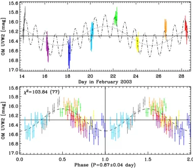
Fig. 5. Weekly and daily UV variability of AA Tau observed with
the OM. Top panel: the dotted and dashed-dotted line show the weekly modulation of the UV flux attributed to the eclipse pe-riod (8.22 days), and the overall modulation of the UV flux. The horizontal line shows the average flux. Bottom panel: the dashed line shows the daily modulation of the UV folded in phase after subtraction of the weekly modulation. Symbols are the same in both panels. The formula of the overall fit (dashed-dotted line) is given by Eq. 1.
reproduced with this simple model including only weekly vari-ations. A Lomb periodogram of the residuals suggests the pres-ence of an additional (high-frequency) modulation with a period of 0.87 ± 0.03 day.
We then compute a grid of fits in the amplitude and phase parameter space to look for optimized values that maximize the peak of the periodogram residuals. This is equivalent to a simul-taneous fitting of both modulations with the long-term period is fixed. We find a better fit (χ2 = 103.8 for 77 d.o.f.). Given the new and old values of χ2and number of degrees of freedom, a F-test indicates a probability of ∼10−11for the null hypothesis; therefore, we conclude that it is reasonnable to add this extra modulation to improve the fit. Moreover, a Lomb periodogram of the residuals shows no other modulations, and a perfect sub-straction of the two modulations. The fit formula is given by the following equation:
UV = 16.30 ± 0.02 mag (1)
+ (0.20 ± 0.02) cos{2π[t − (17.2 ± 0.1)]/8.22}
+ (0.24 ± 0.02) cos{2π[t − (14.75 ± 0.02)]/(0.87 ± 0.04)}, where t is the day in February 2003, and the errors are given at the 68% confidence level.
The top panel of Fig. 5 shows the UV light curve and the fit given by Eq. 1. The bottom panel shows the UV light curve folded in phase with the high-frequency period after the sub-straction of the long-term modulation. This light curve looks rather convincing. However, a longer UV observation with the OM is necessary to have a definitive confirmation of this high-frequency period, which would suggest a non-steady accretion.
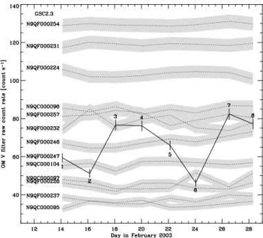
Fig. 6. Optical light curves of the OM guide stars obtained with
the field acquisition exposure. The dashed lines and grey stripes indicate the raw count rates of guide stars and one-sigma vari-ations, respectively. The thick line and error bars shows the op-tical light curve of AA Tau. Labels indicate counterparts in the Guide Star Catalog (version 2.3.2).
2.5.3. Optical variability from the field acquisition exposure We propose here to obtain extra informations on the optical pho-tometry of the target thanks to the OM Field Acquisition expo-sures (FAQs), where several stars are also detected in optical in the OM field of view, and are then available as comparison stars for variability study.
The FAQ is a short exposure (10 s) V-filter image always taken at the start of each science observation (i.e., at the begin-ning of the MOS observation) to allow proper identification of guide stars and to compensate small pointing errors. A threshold-ing is applied to the FAQ image by the OM on board software to identify guide stars. The derived offset is then applied to the OM science windows. The informations (positions in detector coordinates, count rates,...) on the guide stars are reported in the *OMS40000RFX*data files delivered with the Observation Data Files (ODFs). The use of the FAQ image, instead of scheduling an additional OM exposure in the imaging mode default with the
V-filter, allowed us to make a twice longer observation with the
UVW2 filter, by saving at least 5 × 800 s (without taking into account time overheads).
In each observation, we recover sky coordinates from detec-tor coordinates, and identify the counterparts of guide stars in the Guide Star Catalog (version 2.3.2). Then, we build a light curve for the 13 guide stars (including AA Tau). Fig. 6 shows the variations of the raw count rates in the optical of the guide stars during our campaign. All guide stars, except AA Tau, ex-hibited small (lower than 2σ) relative variations in the optical. By contrast, AA Tau exhibited large relative variations, in par-ticular, during observations #1, #2, #5, and #6 where a large dip is visible. We conclude that these 4XMM-Newtonobservations were likely made during the optical eclipses of AA Tau.
Table 3. Journal of ground-based optical observations.
Feb. 2003 Site Tel. Observer Nobs
(d)
13.89–28.88 Teide (Spain) 0.8 m M.R. Z. 177 16.83–17.96 Sierra Nevada (Spain) 1.5 m M. F. 5 20.63–28.64 Mt Maidanak (Uzbek.) 0.5 m K. G. 8
3. UV and X-ray variabilities versus rotational phase 3.1. Ground-based optical photometry
The Journal of ground-based optical observations is given in Table 3. Observations were carried out from three sites over a time span of two weeks, covering ourXMM-Newton observa-tions in February 2003, using either CCD detectors or a pho-tomultiplier tube (Mt Maidanak). Measurements were obtained in the V filter. Differential photometry was performed on CCD images and absolute photometry from photomultiplier observa-tions, with an accuracy of the order of 0.01 mag. Somewhat larger systematic errors (≤0.05 mag) might result from the rel-ative calibration of the photometry between sites. All data re-duction procedures can be found in Bouvier et al. (2003).
The top panel of Fig. 7 shows the ground-based optical light curve; for comparison purpose, the other panels show the UV and X-ray light curves, and the plasma parameters. Unfortunately, due to bad weather conditions in Europe, none ground telescope was able to obtain simultaneous optical obser-vations withXMM-Newton. In the most favorable cases, ground optical photometry was obtained only 4.3 h, 3.1 h, 2.8 h, and 2.0 h before the beginning of the MOS observations #1–#4, re-spectively; and only 3.3 h after the end the last MOS observa-tion. Despite the limited time sampling, a dip, likely associated with a primary eclipse of AA Tau, is however detected at the beginning of the monitoring campaign. This supports what we deduced previously in Sect. 2.5.3 from the optical FAQ images, thatXMM-Newtonobservations #1 and #2 were obtained dur-ing the eclipse. Consequently, the FAQ images can also be used safely to identify an eclipse duringXMM-Newtonobservations #5 and #6, located within the Feb. 23–27, 2003 gap of the ground observation.
3.2. Folded light curves and eclipse phases
To obtain a better determination of the dates of the optical eclipses, we compare our photometry with the one obtained just 6 months apart, from Aug. 27 to Oct. 24, 2003 (Bouvier et al. 2007a). The top panel of Fig. 8 shows both photometry data set folded together in phase using the 8.22-day rotational pe-riod (Bouvier et al. 2007a), i.e., we introduced no phase differ-ence between the two data set. The (arbitrary) common origin of phase was chosen to match the light curve of season 2003 shown in Fig. 15 of Bouvier et al. (2007a), taking the eclipse center at phase 0.5.
The behaviour of our photometry is consistent with the shape of the light curve observed during the season 2003. We can ex-clude any phase offset larger than 0.05 between the two epochs. A deep primary eclipse (∆V ∼ 1.5 mag) is well detected at the beginning of our monitoring campaign. There is also some ev-idence for a shallow secondary eclipse detected only at the end of our monitoring campaign, after the last XMM-Newton ob-servation. The differences in brightness of about 0.5 and 1 mag between the Feb. and Aug. 2003 data, observed at the begin-ning and the end of the primary eclipse, respectively, can be
Fig. 7. Light curves and plasma parameters of AA Tau. The panels show from top to bottom: the optical, UV, and X-ray light curves
(labels indicate observation numbers); the variations of the plasma emission measure(s) and temperature(s), and the photoelectric absorption (Table 2). The top horizontal axis indicates the corresponding phase for the rotation period of 8.22 days. The (arbitrary) phase origin is from Bouvier et al. (2007a).
Fig. 8. Light curves and plasma parameters of AA Tau folded in phase with the rotation period of 8.22 days. Symbols and the phase
origin are identical to the ones used in Fig. 7. In the top panel, black dots show for comparison the optical ground monitoring from Aug. 27 to Oct. 24, 2003 (Bouvier et al. 2007a). The horizontal arrow shows our estimate of the eclipse phase based on the optical ground monitoring.
explained with a longer duration of the eclipse in Feb. 2003. The brightening on Feb. 16, 2003, close to the center of the pri-mary eclipse, was observed with a high sampling rate (∼ 2 min), and exhibited only a fast decay. Therefore, this event is similar to the transient brightening events usually observed in the faint state of AA Tau (Bouvier et al. 1999). The primary eclipses were centered on Feb. 15.5 and Feb. 23.5, 2003, and covered phases ranging from ∼0.3 to ∼0.7. Our ground-based monitoring con-firms thatXMM-Newtonobservations #1, #2, #5, and #6 were made during primary eclipses. In particular, observations #2 and #6 are secured close to the center of the primary eclipse. We can exclude a secondary eclipse at the start of observations #4 and #8 thanks to the FAQ, and moreover the corresponding X-ray light curves show no decay. Therefore, we conclude that the shallow secondary eclipse likely started after the end of our observations. The UV flux is the highest when the primary eclipse starts and the lowest towards the end of it. Indeed, the lowest UV flux was observed during the XMM-Newtonobservation #3 at the end of the egress phase, i.e., outside the primary eclipse. Our model of the UV flux variations helps to disentangle weekly modulation (produced by the warped disk) and daily variation. Eq. 1 indicates that the weekly modulation was at minimum on Feb. 17.2, 2003 (see also the top panel fo Fig. 5), which cor-responds to a phase delay of about 0.2 compared to the opti-cal eclipse. Therefore, the warped disk produces a maximum of obscuration of the UV flux at the end of the optical eclipse. Consequently, the true maximum of the UV flux occurred around phase 0.2, well before the start of the eclipse. We didn’t sur-vey this time interval with XMM-Newton, but we note that a brightening in the B-band of AA Tau was observed around phase 0.2 during the 1995 campaign (Bouvier et al. 1999). The delay between the optical and UV eclipse, and the smaller depth of the UV eclipse (∆UVW2 ∼ 0.40 mag) compared to the optical eclipse (∆V ∼ 1.5 mag), suggests atrailingaccretion funnel flow, producing a strong absorption of the UV photons emitted at the accretion shock.
No eclipses are detected in X-rays. The variable photoelec-tric absorption of the X-ray spectra is not correlated with the rotational phase; similar low and high values of the column den-sity are observed both during the eclipse and outside it. The maximum of the column density was observed at phase 0.6, close to the center of the optical eclipse, during the X-ray flare. However, increases of the column density were also reported during large stellar flares, and solar flares are sometimes associ-ated with coronal mass ejection (see the review on X-ray astron-omy of stellar coronae by G¨udel 2004, and references therein). Therefore, we cannot rule out that the peak of column density is due to this energetic event. The gas column density on the line of sight produced by the warped disk is around 1025cm−2 (Bouvier et al. 1999), which is large enough to absorb all the X-rays emitted by AA Tau, even during a bright and hot flare. The lack of eclipses in X-rays indicates that X-ray emitting regions are located above the high-density disk warp at high latitudes.
The online Fig. 9 shows the scattered plot of the average OM count rate versus the column density, where the count rate error include the observed variations of the UV flux (see Fig. 1). The correlation coefficient of this sample is −0.72, suggesting a true correlation between the two physical parameters as argued by SR, who used smaller error bars for the count rates. However, we note that the data obtained outside the eclipse are located within the cloud of points, with error bars covering all the range of ob-served values of column density and count rate. Therefore, the column density variation cannot be attributed to the disk warp.
Assuming a frequency of one X-ray flare per 650 ks, as ob-served in young solar-mass stars (Wolk et al. 2005), our 38.8 h-exposure should detect only 0.2 flare from AA Tau. The center of the optical eclipse is limited to about 0.2 in phase. Therefore, the combined probability to observe by chance an X-ray flare during the center of the transit of an accretion funnel flow is only 0.04. Moreover, the median flare level in young solar-mass stars is only 3.5 times the characteristic level (Wolk et al. 2005), whereas we observed a flare with a larger amplitude. This sug-gests that this event is associated with the magnetic area corre-sponding to the base of the dipolar magnetic field line, which controls the accretion funnel flow.
4. Discussion and conclusions
The high throughput ofXMM-Newtonallows us to obtain spec-tra of AA Tau at each phase of its activity. By conspec-trast to previ-ousROSATobservations, where the measurement for this source was limited to count rate and hardness ratios in the soft X-ray en-ergy band9, the plasma parameters can be derived from spectral fitting, which provides, in particular, a better measurement of the column density and the X-ray luminosity.
We find that the column density, derived from the photo-electric absorption of the X-rays emitted by the active corona of AA Tau, varies from NH∼ 1.0 × 1022cm−2to 1.8 × 1022cm−2. However, the optical extinction of AA Tau by the dust is very low with AV = 0.78 mag (Bouvier et al. 1999), which can be converted to NH ∼ (1.2 ± 0.1) × 1021cm−2, using the relation
NH/AJ = (5.6 ± 0.4) × 1021cm−2mag−1 (Vuong et al. 2003), combined with the extinction law of Rieke & Lebofsky (1985),
AJ = 0.282 × AV(for their adopted RVvalue of 3.1). We con-clude that there is an excess of column density, varying from 0.9 × 10²² to 1.7 × 1022cm−2. These values are consistent with the one reported by SR. To explain this excess of column density, SR introduced an additional absorption in a disk wind (with no dust, and cool enough to avoid producing any soft X-ray emis-sion), or a peculiar dust grain distribution with RV∼ 0.4 to rec-oncile the observed extinction and X-ray absorption. However, we note that three-dimensional MHD simulations of disk accre-tion to a rotating magnetized star (e.g., Romanova et al. 2003) show that the stellar magnetosphere is far to be an empty cav-ity. Matter accretes mainly through narrow funnel loaded with high-density material (∼1012cm−3), which are surrounded by lower density funnel flows that blanket nearly the whole mag-netosphere. Therefore, we propose to identify this excess of gas with this lower density funnel flows filling the stellar magne-tosphere. Dividing the excess column density by the width of the magnetosphere of AA Tau (about 7.8 stellar radii) leads to a density of a few 1010cm−3, which is compatible with this inter-pretation. Moreover, the multiple spirals visible in the simulated accretion flows should help to produce a variable column den-sity. This low density gas, located below the radius of dust sub-limation (close to the inner accretion disk for AA Tau), is then dust free.
9 To convert theROSAT count rate of AA Tau to X-ray luminosity,
Neuh¨auser et al. (1995) estimate an energy conversion factor from the visual extinction (converted to foreground hydrogen column density) and the second hardness ratio (sensitive to the plasma temperature). This leads to an X-ray luminosity of 0.4 × 1030erg s−1(see Table 1 of
Johns-Krull 2007), which is likely underestimated by a factor of ten (see our simulations of count rates in Sect. 2.4), because the column density of AA Tau (see Table 2, and discussion below) is about 10 times larger than the one assumed by Neuh¨auser et al. (1995).
Accreting TTSs show in average a LX/Lbol ratio 2.5 times smaller than in non-accreting TTSs (see for COUP and XEST re-sults, Preibisch et al. 2005 and Briggs et al. 2007, respectively). This is generally interpreted as a direct or indirect consequence of the accretion process (see discussion in Preibisch et al. 2005; Telleschi et al. 2007; Gregory et al. 2007). The median value of log(LX/Lbol) for AA Tau is −3.5; for comparison this value is in-termediate between −3.7 and −3.3, the median values found for accretors and non-accretors, respectively (Preibisch et al. 2005; Briggs et al. 2007). The peculiar orientation of AA Tau may help to overcome partly the extinction by the accretion funnels (Gregory et al. 2007).
Recently, Johns-Krull (2007) reported new magnetic field measurements for CTTSs, based on Zeeman broading of pho-tospheric absorption lines in the near-IR, showing that the ob-served mean magnetic field is in all cases greater than the field predicted by pressure equipartition arguments. Johns-Krull (2007) suggests that the very strong fields decrease on these stars the efficiency with which convective gas motions in the photo-sphere can tangle magnetic loops in the corona. For AA Tau, Johns-Krull (2007) reports a value of 2.78 kG for the mean mag-netic field, that is 2.7 times larger than the field strength at pressure equipartition; and predicts from solar scaling an (un-observed) X-ray luminosity of about 4 × 1030 erg s−1(for com-parison this value is 10 times greater than the minimum level that we observed). However, our observation shows that a bright X-ray flare can occur during the transit of an accretion funnel flow, and locate the active X-ray area likely close to the foot of the accretion funnel flow. We speculate that a magnetic interac-tion exists between the free falling accreinterac-tion flow and the strong magnetic field of the stellar corona, which may trigger magnetic reconnections and give rise to bright X-ray flares, which boost the X-ray emission.
This campaign of observations of AA Tau with XMM-Newton shows that X-ray spectroscopy with CCD provides a unique tool to probe the circumstellar dust-free gas in this ob-ject, and that some magnetic flares are likely associated with the accretion process. Longer coordinated optical and X-ray/UV ob-servations of AA Tau are still needed to obtain continuous light curves, which is crucial to confirm the flaring behaviour of ac-tive regions associated with the accretion funnel flow, and daily modulation of the UV flux. Simultaneous Zeeman-Doppler im-ages would help to derive a surface magnetogram; this map of the magnetic active regions on the stellar photosphere, combined with the X-ray light curves, would then allow to build a self-consistent three-dimensional model of the corona of AA Tau.
Taking into account that the duration of the visibility window for AA Tau is about 130 ksec perXMM-Newtonorbit (2 days), a full monitoring of two optical eclipse periods of AA Tau (8.22 days) withXMM-Newtonis equivalent to an effective exposure of 1.1 million seconds. This project has the typical duration of the large programs which are anticipated withXMM-Newtonfor the next decade.
Acknowledgements. This research is based on observations obtained with
XMM-Newton, an ESA science mission with instruments and contributions directly funded by ESA Member States and NASA. M.F. was supported by the Spanish grants AYA2004-05395 and AYA2004-21521-E. This research was partly based on data obtained at the 1.5 m telescope at the Sierra Nevada Observatory, which is operated by the Consejo Superior de Investigaciones Cient´ıficas through the Instituto de Astrof´ısica de Andaluc´ıa.
References
Anders, E. & Grevesse, N. 1989, Geochim. Cosmochim. Acta, 53, 197
Argiroffi, C., Maggio, A., & Peres, G. 2007, A&A, 465, L5
Asplund, M., Grevesse, N., & Sauval, A. J. 2005, in ASP Conf. Ser. 336: Cosmic Abundances as Records of Stellar Evolution and Nucleosynthesis, ed. T. G. Barnes, III & F. N. Bash, 25–39
Audard, M., Skinner, S. L., Smith, K. W., G ¨udel, M., & Pallavicini, R. 2005, in Proceedings of the 13th Cambridge Workshop on Cool Stars, Stellar Systems and the Sun, ESA SP-560, ed. F. Favata et al., 411–415
Bouvier, J., Alencar, S. H. P., Boutelier, T., et al. 2007a, A&A, 463, 1017 Bouvier, J., Alencar, S. H. P., Harries, T. J., Johns-Krull, C. M., & Romanova,
M. M. 2007b, in Protostars and Planets V, ed. B. Reipurth, D. Jewitt, & K. Keil, 479–494
Bouvier, J., Chelli, A., Allain, S., et al. 1999, A&A, 349, 619
Bouvier, J., Grankin, K. N., Alencar, S. H. P., et al. 2003, A&A, 409, 169 Briggs, K. R., G ¨udel, M., Telleschi, A., et al. 2007, A&A, 468, 413 Broos, P. S., Feigelson, E. D., Townsley, L. K., et al. 2007, ApJS, 169, 353 Dorman, B. & Arnaud, K. A. 2001, in ASP Conf. Ser. 238: Astronomical Data
Analysis Software and Systems X, ed. F. R. Harnden, Jr., F. A. Primini, & H. E. Payne, 415–418
Favata, F., Flaccomio, E., Reale, F., et al. 2005, ApJS, 160, 469 Feigelson, E. D. & Montmerle, T. 1999, ARA&A, 37, 363
Getman, K. V., Feigelson, E. D., Grosso, N., et al. 2005a, ApJS, 160, 353 Getman, K. V., Flaccomio, E., Broos, P. S., et al. 2005b, ApJS, 160, 319 Gregory, S. G., Wood, K., & Jardine, M. 2007, ArXiv e-prints, 704
Grosso, N., Audard, M., Bouvier, J., Briggs, K. R., & G ¨udel, M. 2007, A&A, 468, 557
Grosso, N., Montmerle, T., Feigelson, E. D., & Forbes, T. G. 2004, A&A, 419, 653
G ¨udel, M. 2004, A&A Rev., 12, 71
G ¨udel, M., Arzner, K., Audard, M., & Mewe, R. 2003, A&A, 403, 155 G ¨udel, M., Audard, M., Magee, H., et al. 2001, A&A, 365, L344 G ¨udel, M., Briggs, K. R., Arzner, K., et al. 2007a, A&A, 468, 353 G ¨udel, M., Skinner, S. L., Mel’Nikov, S. Y., et al. 2007b, A&A, 468, 529 Guenther, E. W., Lehmann, H., Emerson, J. P., & Staude, J. 1999, A&A, 341,
768
G ¨unther, H. M., Schmitt, J. H. M. M., Robrade, J., & Liefke, C. 2007, A&A, 466, 1111
Imanishi, K., Nakajima, H., Tsujimoto, M., Koyama, K., & Tsuboi, Y. 2003, PASJ, 55, 653
Jansen, F., Lumb, D., Altieri, B., et al. 2001, A&A, 365, L1 Johns-Krull, C. M. 2007, ApJ, 664, 975
Johns-Krull, C. M., Valenti, J. A., & Koresko, C. 1999, ApJ, 516, 900 Johns-Krull, C. M., Valenti, J. A., & Saar, S. H. 2004, ApJ, 617, 1204 Kastner, J. H., Huenemoerder, D. P., Schulz, N. S., Canizares, C. R., &
Weintraub, D. A. 2002, ApJ, 567, 434
Kenyon, S. J., Dobrzycka, D., & Hartmann, L. 1994, AJ, 108, 1872 Mason, K. O., Breeveld, A., Much, R., et al. 2001, A&A, 365, L36
M´enard, F., Bouvier, J., Dougados, C., Mel’nikov, S. Y., & Grankin, K. N. 2003, A&A, 409, 163
Morrison, R. & McCammon, D. 1983, ApJ, 270, 119
Ness, J.-U., G ¨udel, M., Schmitt, J. H. M. M., Audard, M., & Telleschi, A. 2004, A&A, 427, 667
Neuh¨auser, R., Sterzik, M. F., Schmitt, J. H. M. M., Wichmann, R., & Krautter, J. 1995, A&A, 297, 391
Ozawa, H., Grosso, N., & Montmerle, T. 2005, A&A, 429, 963
Porquet, D., Mewe, R., Dubau, J., Raassen, A. J. J., & Kaastra, J. S. 2001, A&A, 376, 1113
Preibisch, T., Kim, Y.-C., Favata, F., et al. 2005, ApJS, 160, 401
Reale, F., Betta, R., Peres, G., Serio, S., & McTiernan, J. 1997, A&A, 325, 782 Rieke, G. H. & Lebofsky, M. J. 1985, ApJ, 288, 618
Robrade, J. & Schmitt, J. H. M. M. 2006, A&A, 449, 737
Romanova, M. M., Ustyugova, G. V., Koldoba, A. V., Wick, J. V., & Lovelace, R. V. E. 2003, ApJ, 595, 1009
Scargle, J. D. 1998, ApJ, 504, 405
Schmitt, J. H. M. M. & Favata, F. 1999, Nature, 401, 44
Schmitt, J. H. M. M., Ness, J.-U., & Franco, G. 2003, A&A, 412, 849 Schmitt, J. H. M. M. & Robrade, J. 2007, A&A, 462, L41
Schmitt, J. H. M. M., Robrade, J., Ness, J.-U., Favata, F., & Stelzer, B. 2005, A&A, 432, L35
Smith, K., Audard, M., G ¨udel, M., Skinner, S., & Pallavicini, R. 2005, in Proceedings of the 13th Cambridge Workshop on Cool Stars, Stellar Systems and the Sun, ESA SP-560, ed. F. Favata et al., 971–975
Stassun, K. G., van den Berg, M., & Feigelson, E. 2007, ApJ, 660, 704 Stelzer, B. & Schmitt, J. H. M. M. 2004, A&A, 418, 687
Str¨uder, L., Briel, U., Dennerl, K., et al. 2001, A&A, 365, L18
Telleschi, A., G ¨udel, M., Briggs, K. R., Audard, M., & Scelsi, L. 2007, A&A, 468, 443
Turner, M. J. L., Abbey, A., Arnaud, M., et al. 2001, A&A, 365, L27 Vuong, M. H., Montmerle, T., Grosso, N., et al. 2003, A&A, 408, 581
Walter, F. M. & Kuhi, L. V. 1981, ApJ, 250, 254 Walter, F. M. & Kuhi, L. V. 1984, ApJ, 284, 194
Wang, J., Townsley, L. K., Feigelson, E. D., et al. 2007, ApJS, 168, 100 White, N. E., Giommi, P., & Angelini, L. 1996, VizieR Online Data Catalog Wilms, J., Allen, A., & McCray, R. 2000, ApJ, 542, 914
Wolk, S. J., Harnden, F. R., Flaccomio, E., et al. 2005, ApJS, 160, 423 Yang, H., Johns-Krull, C. M., & Valenti, J. A. 2005, ApJ, 635, 466
N. Grosso et al.: Enhanced X-ray emission from AA Tau, Online Material p 2
Appendix A: Elemental abundances of the coronal plasma and the absorbing material
The typical values of plasma element abundances observed in the coronae of young stars with fine X-ray spectroscopy (G¨udel et al. 2007a), that we use for the vapec coronal plasma model in our X-ray spectral fitting with XSPEC, are given in Col. (2)–(4) of Table A.1.
The column density of the absorbing material located on the line of sight is estimated from spectral fitting using a photoelec-tric absorption model, that uses photoionization cross sections, and solar abundances for the material composition. The wabs photoelectric absorption model use photoionization cross sec-tions of Morrison & McCammon (1983), and (old) solar abun-dances of Anders & Grevesse (1989). Significant revisions of the solar abundances have been made recently, as a result of the ap-plication of a time-dependent, 3D hydrodynamical model of the solar atmosphere, instead of 1D hydrostatic models. This has de-creased the metal abundances, in particular of carbon and oxy-gen, which are the main contributor to the photoionization cross section above 0.3 and 0.6 keV, respectively. Consequently, the absolute value of the column density is dependent of the adopted photoelectric absorption model. Using updated solar abundances is then crucial when the absolute value of the column density is needed (e.g., Vuong et al. 2003). Col. (5)–(7) of Table A.1 give the recent compilation of elemental solar abundances by Asplund et al. (2005), where the decrease of metal by compari-son with Anders & Grevesse (1989) is indicated in the last col-umn.
We test the impact of these udpated solar abundances on our fitting by replacing wabs by tbvarabs (Wilms et al. 2000), which allows to input new abundances for the absorbing ma-terial. Moreover, tbvarabs uses also updated photoionization cross sections. We find nearly identical values of temperature and emission measure, however, as anticipated the column den-sity value is increased. Fig. A.1 shows that column denden-sity val-ues obtained with wabs are underestimated by about 50%.
Fig. A.1. Comparison of the column density values obtained
from spectral fitting when using the old (Anders & Grevesse 1989) and the updated (Asplund et al. 2005) solar abundances. The dashed line shows the mean average between the two values of column density.
Table A.1. Elemental abundances of the coronal plasma and the
absorbing material.
Coronal plasmaa Absorbing materialb
El A(El) n(El)/n(H) angr A(El) n(El)/n(H) angr (1) (2) (3) (4) (5) (6) (7) He 10.99 9.77E-02 1.000 10.93 8.51E-02 0.871 C 8.21 1.63E-04 0.450 8.39 2.45E-04 0.676 N 7.95 8.83E-05 0.788 7.78 6.03E-05 0.538 O 8.56 3.63E-04 0.426 8.66 4.57E-04 0.537 Ne 8.01 1.02E-04 0.832 7.84 6.92E-05 0.562 Na . . . 6.17 1.48E-06 0.691 Mg 7.00 9.99E-06 0.263 7.53 3.39E-05 0.892 Al 6.17 1.47E-06 0.500 6.37 2.34E-06 0.795 Si 7.04 1.10E-05 0.309 7.51 3.24E-05 0.912 S 6.83 6.76E-06 0.417 7.14 1.38E-05 0.852 Cl . . . 5.50 3.16E-07 1.682 Ar 6.30 2.00E-06 0.550 6.18 1.51E-06 0.417 Ca 5.65 4.47E-07 0.195 6.31 2.04E-06 0.892 Cr . . . 5.64 4.37E-07 0.902 Fe 6.96 9.13E-06 0.195 7.45 2.82E-05 0.602 Co . . . 4.92 8.32E-08 0.967 Ni 5.54 3.47E-07 0.195 6.23 1.70E-06 0.954 Notes: Col. (2) and (5) give the element abundances on the logarithmic astronomical scale, where the numbers of hydrogen atoms are set to
A(H) = log n(H) = 12. The numbers of element atoms normalized to
the number of hydrogen atoms are given in Col. (3) and (6); Col. (4) and (7) compare this ratio to Anders & Grevesse (1989)’s photospheric abundances.
a Elemental abundances observed in the coronae of young stars with
fine X-ray spectroscopy (G¨udel et al. 2007a) used in vapec.
b Elemental solar abundances of Asplund et al. (2005) used in tbvarabs.
List of Objects
‘AA Tau’ on page 1
Fig. 2. A subset of X-ray flares from theChandra Orion Ultradeep Projectwith peak amplitude and duration larger than the one observed in AA Tau. The left panels show COUP light curves (see Getman et al. 2005b), where blue and red segments indicate the minimum (BBmin) and maximum (BBmax) levels obtained from Bayesian block analysis (Scargle 1998), respectively. The blue dotted line show the minimum level. The peak amplitudes are also given. The dashed green lines start 1.7 days after the end of the maximum Bayesian block, and indicate the level (2.5 times above the minimum level), that was observed in the third observation of AA Tau. The right panels are an enlargement of the light curve around the Bayesian block showing the peak level and duration. Dots mark the arrival times of individual X-ray photons with their corresponding energies given on the right-hand axis. Large vertical gray stripes indicate the five passages ofChandrathrough the van Allen belts where ACIS was taken out of the focal plane and thus was not observing Orion.
N. Grosso et al.: Enhanced X-ray emission from AA Tau, Online Material p 4
Fig. 3. EPIC pn (black), MOS1 (red), MOS2 (green) spectra of AA Tau plotted with the same scale. The lines show our best fits
using one-temperature plasma combined with photoelectric absorption for observations #1 to #8 (Table 2) from left to right and top to bottom. The residuals are plotted in terms of sigmas with error bars of size one.
Fig. 9. Average OM count rate versus column density. Labels indicateXMM-Newtonobservations. The crosses mark observa-tions obtained outside the optical eclipse. The dotted hourglass shows the column density of observation #2 when using only one-temperature plasma.