HAL Id: hal-00297653
https://hal.archives-ouvertes.fr/hal-00297653
Submitted on 14 Nov 2007
HAL is a multi-disciplinary open access
archive for the deposit and dissemination of
sci-entific research documents, whether they are
pub-lished or not. The documents may come from
teaching and research institutions in France or
abroad, or from public or private research centers.
L’archive ouverte pluridisciplinaire HAL, est
destinée au dépôt et à la diffusion de documents
scientifiques de niveau recherche, publiés ou non,
émanant des établissements d’enseignement et de
recherche français ou étrangers, des laboratoires
publics ou privés.
continental tundra site in the Indigirka lowlands, NE
Siberia
M. K. van der Molen, J. van Huissteden, F. J. W. Parmentier, A. M. R.
Petrescu, A. J. Dolman, T. C. Maximov, A. V. Kononov, S. V. Karsanaev, D.
A. Suzdalov
To cite this version:
M. K. van der Molen, J. van Huissteden, F. J. W. Parmentier, A. M. R. Petrescu, A. J. Dolman, et
al.. The growing season greenhouse gas balance of a continental tundra site in the Indigirka lowlands,
NE Siberia. Biogeosciences, European Geosciences Union, 2007, 4 (6), pp.985-1003. �hal-00297653�
www.biogeosciences.net/4/985/2007/ © Author(s) 2007. This work is licensed under a Creative Commons License.
Biogeosciences
The growing season greenhouse gas balance of a continental tundra
site in the Indigirka lowlands, NE Siberia
M. K. van der Molen1, J. van Huissteden1, F. J. W. Parmentier1, A. M. R. Petrescu1, A. J. Dolman1, T. C. Maximov2, A. V. Kononov2, S. V. Karsanaev2, and D. A. Suzdalov2
1Department of Hydrology and Geo-Environmental Sciences, Faculty of Earth and Life Sciences, Vrije Universiteit Amsterdam, De Boelelaan 1085, 1081 HV Amsterdam, The Netherlands
2Institute of Biological Problems of the Cryolithozone, Russian Academy of Sciences, Siberian Division, 41, Lenin Prospekt, Yakutsk, The Republic of Sakha (Yakutia), 677980, Russian Federation
Received: 13 July 2007 – Published in Biogeosciences Discuss.: 17 July 2007
Revised: 4 October 2007 – Accepted: 29 October 2007 – Published: 14 November 2007
Abstract. Carbon dioxide and methane fluxes were mea-sured at a tundra site near Chokurdakh, in the lowlands of the Indigirka river in north-east Siberia. This site is one of the few stations on Russian tundra and it is different from most other tundra flux stations in its continentality. A suite of methods was applied to determine the fluxes of NEE, GPP, Recoand methane, including eddy covariance, chambers and leaf cuvettes. Net carbon dioxide fluxes were high com-pared with other tundra sites, with NEE=−92 g C m−2yr−1, which is composed of an Reco=+141 g C m−2yr−1 and GPP=−232 g C m−2yr−1. This large carbon dioxide sink
may be explained by the continental climate, that is re-flected in low winter soil temperatures (−14◦C), reducing
the respiration rates, and short, relatively warm summers, stimulating high photosynthesis rates. Interannual variabil-ity in GPP was dominated by the frequency of light limita-tion (Rg<200 W m−2), whereas Recodepends most directly on soil temperature and time in the growing season, which serves as a proxy of the combined effects of active layer depth, leaf area index, soil moisture and substrate availabil-ity. The methane flux, in units of global warming poten-tial, was +28 g C-CO2e m−2yr−1, so that the greenhouse gas balance was −64 g C-CO2e m−2yr−1. Methane fluxes de-pended only slightly on soil temperature and were highly sensitive to hydrological conditions and vegetation compo-sition.
Correspondence to: M. K. van der Molen
(michiel.van.der.molen@falw.vu.nl)
1 Introduction
Tundra covers 8.7×10⁶km2 globally or 6% of the global land area (USGS land use/land cover classification, Ander-son, 1976; van der Molen et al., 2007, 1). Despite this modest area the role of tundra in the global carbon cycle is important: Tundra soils contain an estimated 200 Pg C or about 30% of the global soil carbon pool (Post et al., 1982, Schlesinger, 1999, Hobbie et al., 2000); Global warming is expected (IPCC, 2007) and observed (Serreze et al., 2000, Chapin et al., 2005, Hinzman et al., 2005) to be amplified in polar regions and Northern wetlands (>60◦N) emit ∼8%
of the global natural methane flux (Cao et al., 1998). Being a strong greenhouse gas, increasing methane concentrations are responsible for ∼30% of the enhanced greenhouse effect (Forster et al., 2007). With an estimated carbon dioxide sink of 263 Tg C yr−1 for Russian tundra areas, their role in the global carbon cycle is also substantial (van der Molen et al., 20071). The stability of the tundra carbon pools is thus rele-vant to the global climate. To constrain the fluxes of carbon dioxide and methane, several experiments have been con-ducted in the past decades (cf. Chapin et al., 2000; McGuire et al., 2003). Major conclusions of these experiments are that the fluxes, particularly those of methane, show a high spatial variability due to heterogeneity in topography, veg-etation and hydrology, even at the smallest scales of poly-gons and floodplains (van Huissteden et al., 2005; Kwon et al., 2006). Decomposition of soil carbon is sensitive to tem-perature changes and enhanced thawing (Zimov et al., 2006; Wagner et al., 2007), but growth of tundra ecosystems is 1van der Molen, M. K., Dolman, A. J., Belelli, L., et al.: The carbon balance of Boreal Eurasia consolidated with eddy covariance measurements, in review, 2007.
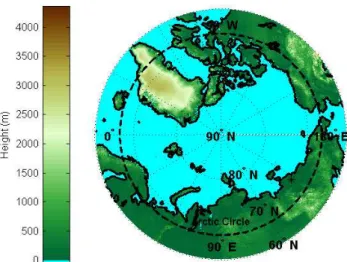
Fig. 1. Circum polar elevation map, the asterisk indicates the
loca-tion of the site.
nitrogen limited, which would reduce the sensitivity to cli-mate warming (Hobbie et al., 1998). The effect of clicli-mate warming in recent decades is already detected in the form of enhanced shrub growth and an advancement of the tree line (Jia et al., 2003; Lloyd et al., 2003; Esper et al., 2004).
The majority of the tundra field experiments were con-ducted on the North slope of Alaska and the Seward Penin-sula in Alaska. The tundra areas in the Russian Federa-tion, which comprise 45% of the total (van der Molen et al., 20071), are much less studied: Heikinnen et al. (2002) re-port about an experiment in Vorkuta, European Russia, Wag-ner et al. (2003) about an experiment in the Lena Delta and Tsuzuyaki et al. (2001) and Corradi et al. (2005) about exper-iments in the floodplains of the Kolyma River near Cherskii. Christensen et al. (1995) performed methane flux measure-ments along a transect through Arctic Siberia via the Arctic Ocean. Other greenhouse gas flux studies were performed on tundra in Sweden (Christensen et al., 2004) and Greenland (Christensen et al., 2000; Friborg et al., 2000; Soegaard et al., 2000). However, climatic and environmental conditions vary considerably across the arctic, as a function of conti-nentality (Sect. 2.1), distance to the northern treeline and the presence of mountain ranges (cf. Lynch et al., 2001).
Here we present the first combined observations of car-bon dioxide and methane fluxes collected at a tundra site in the lowlands of the Indigirka river, near the village of Chokurdakh, in North East Siberia. At about 150 km from East Siberian Sea, the site is located roughly half way be-tween the coast and the tree line. The nearest mountains are about 450 km to the South, making the latitudinal extend of the Indigirka lowlands some 600 km, in comparison with 350 km between the Brooks Range and the Arctic Ocean in Alaska. As such, climate is more continental and less in-fluenced by topography at this site than most other Arctic measuring sites. As 45% of the tundra area lies in the
Rus-Fig. 2. Geomorphological map of the site, derived from field
map-ping and a satellite picture of the Kytalyk reserve on http://maps. google.com (http://maps.google.com/?ll=70.8275,147.4790&spn= 0.1578,0.5905&t=k).
sian Federation, where it is the largest land cover class after forest, this study provides data necessary to understand the carbon dioxide and methane balances of Boreal Eurasia and to put existing tundra field experiment in a circumpolar per-spective.
Carbon dioxide fluxes were measured from 2003 to 2006, continuously during the summer using eddy covariance, complemented with chamber and leaf cuvette measurements of ecosystem respiration and photosynthesis rates. Methane flux measurements were carried out during intensive field ex-periments in the summers of 2004, 2005 and 2006. The ob-jective of this study is to present the seasonal cycle of the car-bon dioxide and methane fluxes, the resulting global warm-ing potential, as well as the annual sums. For a better in-terpretation of the measurements, we perform and validate a partitioning of the net carbon dioxide fluxes into the com-ponents of ecosystem respiration and photosynthesis. We also use and validate the ORCHIDEE photosynthesis model and the PEATLAND-VU methane flux model to scale up the measurements in time and space.
2 Site description and instrumentation
2.1 Site description
The research site (70◦49′36.28′′N, 147◦29′56.23′′E,
10 m a.m.s.l., Fig. 1) is located in the World Wildlife Fund Kytalyk (Crane) reserve, 28 km northwest of the village of Chokurdakh in the Republic of Sakha (Yakutia), Russian Federation. This puts the site roughly half way between the East Siberian Sea (150 km to the North) and the transition zone between taiga and tundra. The site is on the bottom of a thermokarst lake, that was drained by intersection of the Berelekh river, a tributary of the Indigirka river (Fig. 2).
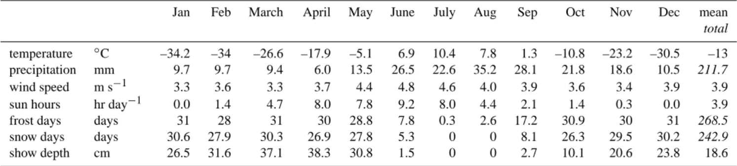
Table 1. Basic climatology of the study site as observed at the weather station near the village of Chokurdakh (WMO station 21946
Chokurdakh) between 1999 and 2006. Snow depths at the field station are usually 60–80 cm. Precipitation is reported for 1994–1999.
Jan Feb March April May June July Aug Sep Oct Nov Dec mean
total
temperature ◦C –34.2 –34 –26.6 –17.9 –5.1 6.9 10.4 7.8 1.3 –10.8 –23.2 –30.5 –13
precipitation mm 9.7 9.7 9.4 6.0 13.5 26.5 22.6 35.2 28.1 21.8 18.6 10.5 211.7
wind speed m s−1 3.3 3.6 3.3 3.7 4.4 4.8 4.6 4.0 3.9 3.6 3.4 3.9 3.9
sun hours hr day−1 0.0 1.4 4.7 8.0 7.8 9.2 8.0 4.4 2.1 1.4 0.3 0.0 3.9
frost days days 31 28 31 30 28.8 7.8 0.3 2.6 17.2 30.9 30 31 268.5
snow days days 30.6 27.9 30.3 26.9 27.8 5.3 0 0 8.1 26.3 29.5 30.2 242.9
show depth cm 26.5 31.6 37.1 38.3 30.8 1.5 0 0 2.7 10.1 20.6 23.8 18.6
2.1.1 Climatology
A basic climatology is presented in Table 1. With a mean January temperatures of −34.2◦C, the Chokurdakh site is colder than at other field sites e.g. near Scoresbysund (North East Greenland), Kiruna (North Sweden) and Vorkuta (East European Russia) (−13 to −16◦C), it is also colder than Barrow (Alaska, −25.4◦C), and Tiksi, at the Lena Delta (−30◦C). Temperatures below −40◦C occur regularly. The mean July temperature of +10.4◦C is warmer than in Barrow (4.6◦C) and Scoresbysund (6.0◦C), comparable to Tiksi and somewhat cooler than Kiruna and Vorkuta (12–14◦C). Max-imum temperatures at the site may reach over +25◦C. The mean annual temperature is −10.5◦C. Monthly mean temper-atures are quite variable in the winter, and more constant in the summer. Annual mean precipitation amounts to 212 mm, of which about half falls as snow. Snow depths at the site are 60–80 cm and quite constant throughout the years, this is somewhat more than measured at the long-term weather station near the village. With wind speeds around 4 m s−1 the site is amongst the calmer sites, Barrow and Vorkuta in particular experience stronger winds (∼5 m s−1). Wind di-rections are distributed fairly even, with a slight preference for northeasterly and southwesterly directions. The average (1998–2006) number of sunshine hours in June, July, August is 275, 248 and 136 h of sun. In 2004, the number of sun-hours in June, July and August was in total 384 h less (128 h per month) and in 2005 it was in total 186 h more (62 h per month). The years 2003 and 2006 had sunshine hours close to the long-term mean.
During the operation years of the site, water level in the nearby river varied considerably, and consequently also on the measurement sites. With respect to 2003, in 2004, the river stage was relatively high after high snowmelt runoff. In 2005, the river stage was approximately 1.5–2 m lower, as a result of a dry winter and spring; moreover, the air tempera-tures were as high as 30◦C during most of the field campaign. The river stage in 2006 was intermediate.
2.1.2 Geology and soils
Three major topographic levels occur around the measure-ment site (Fig. 2). The highest level is underlain by “Ice complex deposits” or “Yedoma”, ice-rich silt deposits of Late Pleistocene, deposited as loess or fluvial silts (Schirrmeis-ter et al., 2002; Gavrilov et al., 2003; Zimov et al., 2006). Near the site, the ice complex deposits occur in terrace-like 20–30 m high hills, probably representing a Pleistocene river terrace surface which has been eroded by thermokarst processes. Presence of cross-bedding in a riverbank expo-sure near the site indicates a fluvial origin of the sediments. The measurement site itself is located in a depression be-tween two N-S trending ice complex remnants, constitut-ing the second topographic level. This depression originated as a thermokarst lake of Holocene age, drained by fluvial erosion. The lowest topographic level is the present river plain, situated 2–3 m below the lake bottom. The river plain has a conspicuous fluvial relief with levees, back swamps and lakes. Active thermokarst features (slumps and thermo-erosional niches) are common along the river bank, and thermo-erosional expansion of creeks and sloughs is also common on the river plain.
The area is underlain by continuous permafrost. The ac-tive layer ranges from 25 cm in dry, peat-covered locations to 40 cm in wet locations. On the floodplain the active layer may be locally thicker. Both on the floodplain and the lake bottom a network of ice wedge polygons occurs, in general of the low-centered type. The ice wedge polygons on the lake bottom have a more mature appearance, with well developed ridges and wet, low centers. This suggests that the age of this surface is older than that of the river plain. Next to the polygons, also low, flat palsa-like features occur on the lake bottom, representing generally drier areas. The lake bottom is drained by a diffuse network of depressions, covered with a Carex-Eriophorum vegetation and underlain by a generally thicker active layer.
The soils generally have a 10–15 cm organic top layer overlying silt. In case of wet sites, the organic layer con-sists of loose peaty material, composed either of sedge roots
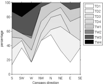
Fig. 3. Areal proportion of vegetation/terrain classes along 150 m
transects in different directions from the tower, TD classes: dry sites with a grass-moss-Betula nana vegetation (TD1,TD3) or
Erio-phorum hummocks (TD2). TD4 is a dried Sphagnum vegeta-tion with very thin active layer. TW classes: wet sites with a
Carex-Eriophorum vegetation (TW1, “sedge meadows”), open
wa-ter (TW2) or Sphagnum-dominated vegetation (TW3,4). See Ta-ble 2 for further description of terrain classes.
or Sphagnum peat, depending on the vegetation. Drier sites tend to have a thinner, more compact organic layer.
The Berelekh river meanders from west to east. In a band of about 30 km wide, centered at the river, many small lakes occur (17%), with diameters of a few hundred meters. In a wider area (about 75×75 km) fewer, larger lakes occur (22%), with typical diameters of 10 km.
Based on a detailed digital map, the fraction of water in the narrow band was estimated at 17% and at 22% in the wider area. The relatively large fraction of water needs to be taken into account when interpreting the flux measurements made on land.
2.1.3 Vegetation composition
On the Circumpolar Arctic Vegetation Map (CAVM Team, 2003) the area and its surroundings classify as G4 (Tussock-sedge, dwarf-shrub, moss tundra) or S2 (Low-shrub tundra). However, within the site and its wide surroundings large tracts of W2 (Sedge, moss, dwarf-shrub wetland) occur and may even dominate. In the area in the immediate surround-ings of the tower, the vegetation is a mosaic of: 1) drier sites (palsa, ridges along ice wedges) dominated by Betula nana,
Salix sp., mosses and grasses; 2) isolated depressions
(poly-gon centers, thawing ice wedges) dominated by submerged
Sphagnum, Potentilla palustris and some Carex, 3) mires
with Sphagnum hummocks and some Salix and 4) depres-sions with a dense Carex-Eriophorum vegetation.
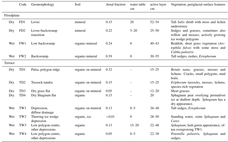
For the methane flux measurements, a classification has been developed, linking vegetation and geomorphology (Van Huissteden et al., 2005; Table 2, Fig. 2). At the highest level, this classification distinguishes between floodplain and river terrace/tundra. Next, dry and wet sites have been dis-tinguished based on water table position, where “wet” is de-fined as largely water saturated soils, with a water table not lower than 5 cm below the surface. The lowest level of the classification is based on smaller morphological features and their vegetation. Van Huissteden et al. (2005) give a detailed description of all classes. The areal fraction of the terrain units has been determined by point counting at regular dis-tances along transects, near the eddy correlation flux tower and on the floodplain area near the field station. In general, in the area to the south and west of the tower, the wet TW classes (see Table 2 for code conventions) dominate while to the north and east of the tower the dry TD classes dominate (Fig. 3). On the floodplain, FW2 dominates.
2.2 Instrumentation
2.2.1 Eddy covariance and micrometeorology
At the site two masts are installed, the first mast contains the eddy covariance instrumentation, consisting of an ultrasonic anemometer (Gill Instruments, Lymington, UK, type R3-50) and an open path infra-red gas analyzer (Licor, Lincoln, NE, USA, type Li-7500) at a height of 4.7 m. Eddy covariance data were collected on a handheld computer (van der Molen et al., 2006) at a rates between 5 and 10 Hz, depending on the time between field visits and storage capacity. It was experi-mentally verified that reducing the data collection frequency to 5 Hz did not significantly change the resulting fluxes at the site. Eddy fluxes were computed on a half-hourly basis following the Euroflux methodology (Aubinet et al., 2000) with the addition of the angle of attack dependent calibra-tion (van der Molen et al., 2004; Nakai et al., 2006). Stor-age flux was corrected for using the discrete approach, which did not significantly change the fluxes however. The second mast contains a shortwave radiometer (Kipp & Zn, Delft, the Netherlands, type albedometer, CM7b), up- and down facing longwave radiometers (The Eppley Laboratory, Newport, RI, USA, type PIR) and a net radiometer (Campbell Scientific, Logan, UT, USA, type Q7). 20 soil thermometers (made at the Vrije Universiteit Amsterdam) were dug into 2 profiles, each reaching 60 cm into the ground. The one profile was in a polygon depression, where the soil is more moist, the other profile was on the rim of a polygon with a relatively low water table. Soil moisture was not measured. Small scale variations in topography in relation to polygon mires causes a rather heterogeneous soil moisture field, however, during the entire growing season, the soil moisture conditions are wet. The instruments were usually installed in April each year and taken down for the winter in October. However, be-cause the system was operated on solar power and batteries,
Table 2. Site classification based on geomorphology, water table position and vegetation. Areal fraction with respect to a 150 m radius circle
around eddy correlation tower for the terrace (T) sites, and on cross transects for the floodplain (F), based on 5 m distance point counts.
Code Geomorphology Soil Areal fraction water table active layer Vegetation, periglacial surface features
cm cm
Floodplain
Dry FD1 Levee mineral 0.15 20 52–54 Tall Salix shrub with moss and lichen
understorey Dry FD2 Levee-backswamp
transition
mineral 0.22 5–20 25–50 Sedges and grasses, sometimes also
willow and mosses; actively growing ice wedge polygons
Wet FW1 Low backswamp organic-mineral 0.24 0 40–43 Reddish, short grass vegetation
(Arc-tophila fulva) with some moss and Caltha palustris
Wet FW2 Backswamp organic-mineral 0.39 0 30–55 Tall sedges, rushes, Eriophorum
Terrace
Dry TD1 Palsa, polygon ridge organic on mineral 0.32 – 15–25 Betula nana, grasses, mosses and lichens. Cracks, small polygons, mud boils.
Dry TD2 Tussock tundra organic on mineral 0.15 – 15–25 Eriphorum tussocks, mosses, lichens, species-rich vegetation
Dry TD3 Dry grass flat organic on mineral 0.05 – 12–20 Short grasses
Dry TD4 Dry Shagnum flat organic 0.15 – 20 Sphagnum peat overlying permafrost
ice at shallow depth. Sphagnum has a dry appearance.
Wet TW1 Depression, diffuse drainage
organic on mineral 0.13 0–5 26–48 Tall sedges, Eriophorum Wet TW2 Thawing ice wedge
depression
organic, ice <0.01 0 28–50 Standing water, some Sphagnum and Carex
Wet TW3 Low polygon centre, other depressions
organic 0.13 15–20 22–48 Sphagnum, lush green appearrance, of-ten overgrowing TW1.
Wet TW4 Low polygon centre, other depressions
organic 0.05 0–5 22–38 Potentilla palustris, Sphagnum and
sedges.
and the area is inaccessible during the period of snow melt and ice breaking (May), power failures caused the system to shut down in the spring of 2004, 2005 and 2006, but each year’s record starts at least within a few days after leaf onset. Low solar radiation conditions cause some gaps in the record during the fall. An additional wind generator was installed in 2006 to help prevent power failures.
2.2.2 Chamber measurements of the ecosystem respiration rate of CO2
Observations of the ecosystem respiration rate were made us-ing a portable gas analyzer (PP Systems, Hitchin, UK, type EGM-4) equipped with a closed chamber (type SRC-1) and a soil temperature probe (type STP-1). The chamber has dimensions of (height × diameter) = (15×10 cm). 25 alu-minium rings on which the chamber fits precisely were in-stalled in the field at various locations with representative vegetation cover, so that the respiration rates were measured each time at the same places without disturbing the soil. The increase in volume was corrected for. Observations were carried out from 27 July to 1 August 2004 (Fig. 7a) and from 26 to 29 June 2005 (Fig. 7b), at 3 hourly intervals. In
2004, 189 individual measurements passed quality control and in 2005, 249. At a few measuring locations, the ecosys-tem respiration rate is possibly under-estimated, because the rings and chambers could not hold larger plants. However, at most of these sites, the plant cover would not be more than a single twig. Some variation of ecosystem respiration rate was observed between the various locations, but the average fluxes per location varied less than a factor 2. The differ-ences were not consistent and variations due to temperature and weather were of similar magnitude. We assumed that the mean ecosystem respiration rate over each of the 25 lo-cations as representative for the ecosystem respiration in the footprint of the flux tower.
2.2.3 Photosynthesis measurements
On 14 July 2003, measurements of photosynthesis rates were made using a portable LCA-4 (ADC Bioscientific, Herts, UK) Infrared Gas Analyser with leaf cuvettes. On 30 July 2004, a LI-6400 system (Li-Cor, Lincoln, NE, USA) was used. The photosynthetic activity was measured of leaves of Betula, Salix, Eriophorum plants. Of each species 2–3 leaves were sampled and the measurements were repeated
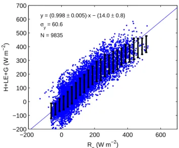
−200 0 200 400 600 −200 −100 0 100 200 300 400 500 600 700 y = (0.998 ± 0.005)⋅x − (14.0 ± 0.8) σy = 60.6 N = 9835 R n (W m −2) H+LE+G (W m −2 )
Fig. 4. Energy balance closure based on half hourly fluxes. The
x-axis indicates the amount of net radiation (Rn) received and the y-axis the amount of energy spent on the sensible (H ), latent (LE) and soil heat fluxes (G).
3–5 times. The entire measurement cycle was repeated at three hour intervals during 24 h periods, using the same leaves. After the last measurement cycle, the leaves were taken to determine the leaf area. No systematic difference in photosynthetic activity was observed between species, and the variation between leaves of the same species was of the same order of magnitude as the variation between species. For this reason the measurements taken in a three hour inter-val were averaged into a single inter-value.
2.2.4 Methane flux measurements
Methane flux measurements were made during a number of consecutive days in the summers of 2004 (27–30 July), 2005 (20–27 July), 2006 (15–18 August). The methane flux mea-surements were made using static chambers (diameter 30 cm, height 20–30 cm), at 55 sites in 2004, 86 sites in 2005 and 60 sites in 2006, selected from the terrain classes in Ta-ble 2 for determination of spatial variation of the fluxes. The round static chambers were attached to a photo-acoustic gas monitor (model 1312, Innova AirTech Instruments, Ballerup, Denmark), capable of measuring CO2, H2O, N2O and CH4 concentrations. In 2006 a model 1412 Innova was used, equipped for H2O and CH4 measurements. The detection limit for CH4is 0.1 ppmv, resulting in a theoretical minimum detectable flux of 0.13 mg CH4m−2hr−1given the measure-ment setup. In total, 201 methane flux measuremeasure-ments have been made during these three field campaigns. For logis-tic reasons, only a few chambers could be transported to the site. To obtain insight in spatial variation of the methane fluxes we choose for measurement of a large number of sites rather than a few fixed measurement stations, as described by
Table 3. Soil characteristics.
component fraction density specific heat kg/m3 kJ/kg/K
mineral 4% 2650.00 0.90
organic 36% 1300.00 1.92
water 30–60% 1000.00 4.18
air remaining 1.20 1.01
Van Huissteden et al. (2005). Installing chambers relatively shortly before measurement could lead to aberrant fluxes due to ebullition. Therefore, a few sites have been measured peatedly during several days; the measured fluxes proved re-peatable. Moreover, each flux measurement was checked for quality by graphing the CH4concentration against time. Ir-regular increase of the CH4concentration was taken as evi-dence of induced ebullition or leakage of the chamber. These measurements were rejected. Each flux measurement was accompanied by determination of the active layer depth and soil temperatures. At each site characteristics of the vegeta-tion and soil profile, and the water table were recorded, using a hand auger. Each flux measurement was quality controlled following van Huissteden et al. (2005).
3 Validation of measurements and models
3.1 Energy balance closure
Figure 4 shows the energy balance closure as a method to test the quality of the eddy flux data. The linear least square re-gression through all data points shows a good energy balance closure of 99.8% with an offset of 14 W m−2and a standard deviation of 60 W m−2. However, the binned data suggest an underestimation of the larger fluxes. The soil heat flux G was estimated here as a function of the change of tempera-ture in the profile and typical soil characteristics as shown in Table 3.
3.2 CO2fluxes during calm conditions
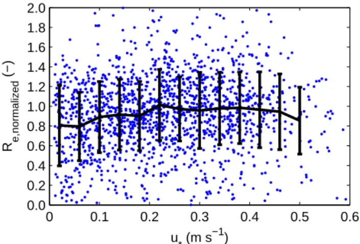
Underestimation of ecosystem CO2fluxes under calm con-ditions is amongst the most prominent error sources of the eddy covariance method. Figure 5 shows some indications that this so-called u∗-problem may occur at the field site for u∗<0.2 m s−1, although the underestimation is small com-pared to what is sometimes observed at other sites (cf. Dol-man et al., 2004). Because calm, “night-time” conditions may also occur during the polar day at this high latitude site, we estimate NEE for u∗<0.2 m s−1as follows:
where Reco,mod and GPPmod are model estimates of the ecosystem respiration and photosynthesis rates (see Sects. 3.3 and 3.5).
3.3 Parameterising the ecosystem respiration rate
Continuous time series of the ecosystem respiration rate was estimated as the CO2 flux measured with eddy covariance under conditions of low global radiation (<20 W m−2)and
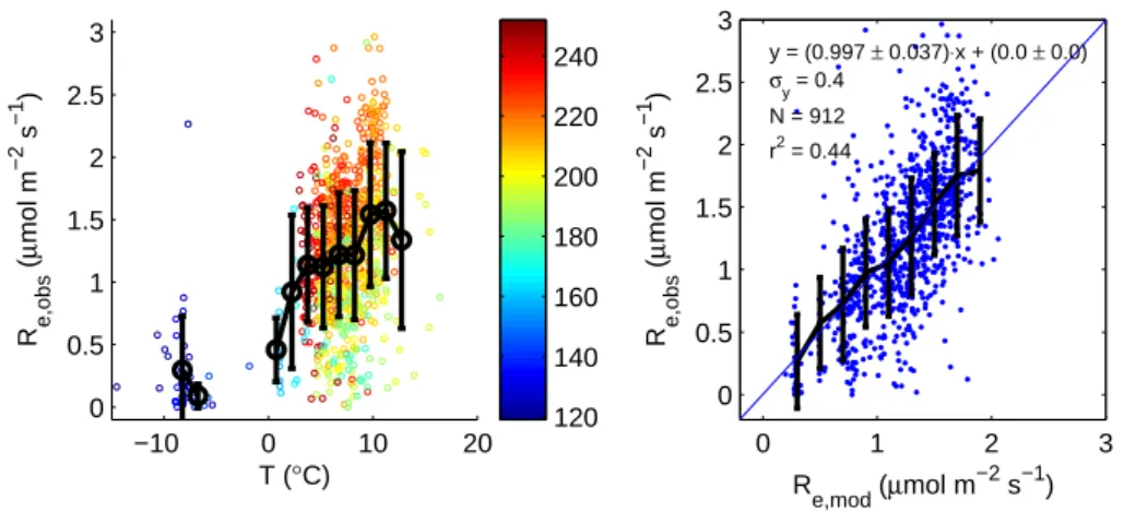
strong turbulence (u∗>0.2 m s−1). Figure 6a shows that the
ecosystem respiration rate increases with temperature, but that soil temperature does not explain all the variation. The timing in the growing season appears to explain a large part of the remaining variation, as indicated by the colours of the data points. A linear optimization of the model
Reco,mod= R0Q(T /10 10) (180 < doy < 240) (2) where the base respiration R0(µmol m−2s−1)is written as a 3rd degree polynomial function of the day-of-year, is shown in Fig. 6b. The optimized parameters are [−8.37E-06, 5.15E-03, −1.04E+00, 6.94E+01] with an associated Q10of 1.80. The rationale for using day-of-year as a proxy for R0is that active layer depth, biomass and substrate co-vary during the growing season and it is as yet impossible to distinguish be-tween those. For dates outside the range 180 to 240, Eq. (2) is fixed to 180 or 240. The resulting Reco,mod has a slope of about 1.0 versus Reco,obs but with considerable scatter (r2=0.44). The unexplained part of the variation may be due to heterogeneity of vegetation composition or ground water table. The respiration rate does not vary with wind direc-tion. The respiration rate derived here from the eddy covari-ance data is compared with the chamber measurements in Sect. 4.2.
3.4 Validation of partitioning of NEE into Recoand GPP The partitioning of NEE as measured by the eddy covariance method into Reco and GPP was validated against chamber and leaf level photosynthesis measurements. Figure 7 shows a comparison of the diurnal cycles of respiration rates result-ing from Eq. (2) with chamber measurements of the respira-tion rate for a few consecutive days in 2004 and 2005. Fig-ure 7 shows agreement in the order of magnitude, but there is also considerable variation. Particularly on days 209 and 210 in 2004 (Fig. 7a), the chamber fluxes are larger than the eddy fluxes, but at these days relatively few reliable chamber mea-surements were made, due to malfunctioning of the battery. From day 211 to 214, when measurements were made at a higher temporal resolution, the agreement is closer. The x’s indicate the variability of eddy covariance flux measurements at the corresponding times, for turbulent (u∗>0.2 m s−1)and dark (Rg<20 W m−2)conditions.
The photosynthesis rate GPP was estimated as Reco–NEE. Diurnal cycles of photosynthesis rates were also measured independently (see Sect. 2). Figure 8 shows a good level of
0 0.1 0.2 0.3 0.4 0.5 0.6 0.0 0.2 0.4 0.6 0.8 1.0 1.2 1.4 1.6 1.8 2.0 u * (m s −1) R e,normalized (−)
Fig. 5. The ecosystem respiration rate, determined from nighttime
(Rg <20 W m−2)eddy covariance measurements, normalized for
temperature and time influences, as a function of u∗, showing a slight underestimation for u∗<0.2 m s−1.
agreement between GPP from the partitioning of eddy fluxes on the one hand and leaf level measurements on the other hand on 14 July 2003 and 30 July 2004. Figure 8 also shows model simulations of GPP, using the ORCHIDEE model that is described in Sect. 3.5. The close agreement in absolute values and in the shape of the diurnal cycles of Recoand GPP gives confidence in the performance of the method of parti-tioning NEE into GPP and Reco.
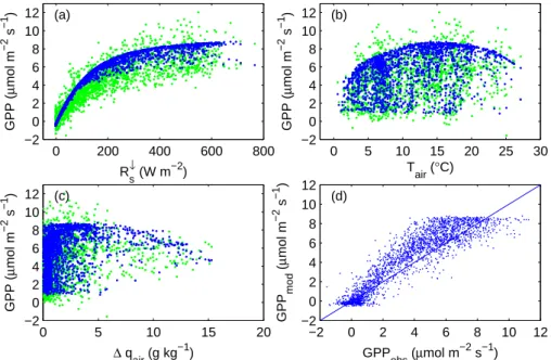
3.5 Modelling of photosynthesis and methane fluxes The ORCHIDEE photosynthesis model (Krinner et al., 2005; Morales et al., 2005) was used in combination with the PEATLAND-VU methane flux model (van Huissteden and van den Bos, 2003; van Huissteden, 2004). ORCHIDEE sim-ulates GPP as a function of solar radiation, surface temper-ature, air humidity, air pressure, CO2concentration and sur-face conductance (Farquhar, 1980; Ball et al., 1987; Collatz et al., 1992). ORCHIDEE may also be used as a dynamical vegetation model, but in this application only the photosyn-thesis module was used, without accounting for phenology. The C3 grassland plant functional type was used to simu-late the tundra photosynthesis rate, after adapting the Vc,max (Vj,max) from 60 (120) to 35 (70). The Leaf Area Index
was maintained at 1.0. The performance of the ORCHIDEE model for tundra is shown in Fig. 9, using mid summer data, when the vegetation was fully developed. Further validation is provided in Fig. 8, where diurnal cycles of simulated GPP are compared with leaf cuvette measurements and with par-titioned eddy covariance measurements. GPP is simulated from 2003 to 2006, for each half hour that the required input variables are available, and is used for gap filling, when me-teorological variables were available and eddy fluxes were not available, or when eddy fluxes were rejected due to low turbulence conditions (Eq. 1).
−10 0 10 20 0 0.5 1 1.5 2 2.5 3 T (°C) R e,obs ( µ mol m −2 s −1 ) 120 140 160 180 200 220 240 0 1 2 3 0 0.5 1 1.5 2 2.5 3 y = (0.997 ± 0.037)⋅x + (0.0 ± 0.0) σy = 0.4 N = 912 R e,mod (µmol m −2 s−1) R e,obs ( µ mol m −2 s −1 ) r2 = 0.44
Fig. 6. (a) the variation of observed ecosystem respiration rate as a function of soil temperature and time. (b) performance of the ecosystem
respiration model.
Fig. 7. Comparison of Reco,obs: observed respiration rate (night-time eddy fluxes when u∗>0.2 m s−1), Reco,mod(Eq. 1), chamber fluxes at individual locations and the mean chamber fluxes. The left figure shows data for 27 July to 1 August 2004 and the right figure for 26 to 29 June 2005.
PEATLAND-VU simulates CH4fluxes as the difference of production in the root zone and consumption by
oxida-21 0 3 6 9 12 15 18 21 0 −2 0 2 4 6 8 10 12 14 time (LT) GPP ( µ mol m −2 s −1 ) eddy flux ORCHIDEE LI−6400 21 0 3 6 9 12 15 18 21 0 −2 0 2 4 6 8 10 12 14 time (LT) GPP ( µ mol m −2 s −1 ) eddy flux ORCHIDEE LI−6400
Fig. 8. Diurnal cycles of GPP determined by 1) partition of eddy
covariance measurements of NEE, 2) model simulations with OR-CHIDEE, using local meteorology and 3) leaf level measurements. The left figure shows the diurnal cycles for 14 July 2003, and the right figure for 30 July 2004.
tion (cf. Walter, 2000). The production is a function of the rate of root exudation of labile organic compounds, which is generally assumed to depend on NPP, as well as a function of the availability of oxygen in the soil. For this purpose, we assume that NPP corresponds to 50% of GPP (Turner et
0 200 400 600 800 −2 0 2 4 6 8 10 12 R s ↓ (W m−2 ) GPP ( µ mol m −2 s −1 ) (a) 0 5 10 15 20 25 30 −2 0 2 4 6 8 10 12 T air (°C) GPP ( µ mol m −2 s −1 ) (b) 0 5 10 15 20 −2 0 2 4 6 8 10 12 ∆ q air (g kg −1 ) GPP ( µ mol m −2 s −1 ) (c) −2 0 2 4 6 8 10 12 −2 0 2 4 6 8 10 12 GPP obs (µmol m −2 s−1) GPP mod ( µ mol m −2 s −1 ) (d)
Fig. 9. Performance of the ORCHIDEE model to simulate GPP as a function of (a) global radiation, (b) air temperature (c) vapour pressure
deficit. The blue dots represent the modelled GPP and the green ones the GPP obtained by partitioning the observed NEE. (d) shows modelled versus observed GPP. In this comparison data only mid summer data have been used (9 July to 18 August), to exclude dates when the vegetation was not fully grown.
al., 2006), or 125% of NEE (which are numerically identi-cal in this instance). The NPP input for PEATLAND-VU is derived from the eddy covariance data, augmented with modelled values from ORCHIDEE whenever gaps in the data were present. Oxidation is a function of soil aeration, which varies with ground water table. The ground water table is modelled as a function of the balance between precipitation and evaporation, which are both observed, and snowmelt, us-ing a modified version (Yurova et al., 2007) of the model of Granberg et al. (1999). The modelling of the water table for the site and the methane flux simulations using the modelled water table are described in a separate publication by Pe-trescu et al. (2007). With PEATLAND-VU, methane fluxes were simulated for three different vegetation types represen-tative for the vegetation around the tower site: Carex vegeta-tions (TW1 type), Sphagnum vegetavegeta-tions (TW3-4 type) and dry tundra vegetation (TD types). The NPP generated from the eddy covariance data or ORCHIDEE was used as input for PEATLAND-VU. This was done for 2004 to 2006, so that the model could be verified with the field observations. It was assumed that the ombrotrophic Sphagnum vegetations and dry tundra vegetations had a lower primary production (20% lower than average NPP) than the TW1 type vegeta-tion (20% higher than average NPP). On wet sites, oxidavegeta-tion is a function of vegetation species, with Carex species hav-ing aerenchyma, which enable efficient transport of methane to the atmosphere, with less oxidation. Sphagnum mosses have a symbiosis with methanotrophic bacteria (Raghoebars-ing et al., 2005), result(Raghoebars-ing in a larger methane oxidation. The
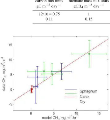
vegetation-related parameters (plant transport rate factor and oxidation factor) in the CH4submodel of PEATLAND-VU have been set accordingly. For the dry sites, water table was set 20 cm lower than for the wet sites, in line with the field observations made during the methane flux measurements. After initial setting of these parameters, the model output was further optimized on both the methane production rate, a tuning parameter in the model (Walter, 2000), and the plant oxidation rate. The performance PEATLAND-VU model for methane fluxes is shown in Fig. 10, where simulated methane fluxes are plotted versus observed ones, for the three differ-ent simulated vegetation types and the three available mea-surement campaigns. Although the uncertainty ranges are quite wide, the actual values compare rather well. This model was used successfully also for methane fluxes in Stordalen, Abisko, Sweden (Petrescu et al., 2007). The methane model was used to scale up the observed fluxes in time to the com-plete length of the growing season for the sites around the flux tower. The wet floodplain (FW) have been modelled by Petrescu et al. (2007) but are not considered here because the data from the floodplain do not permit a consistent compari-son between CO2and CH4fluxes.
3.6 Comparison of carbon dioxide and methane fluxes As the main objective of this paper is to determine the net greenhouse gas budget for this site, it is convenient to express methane fluxes in units of global warming potential. Based on the IPCC 4th Assessment report (Forster et al., 2007),
Table 4. Comparison of units of methane fluxes. The first row gives conversion factors from methane flux in units gCH4m−2day−1to other the units in the other columns. The second row gives conversion factors from units gC-CO2e m−2day−1to units in the other columns. The asterisk-marked column indicates the Global Warming Potential over a 100 year time horizon of gCH4m−2day−1, although these units are not used here.
carbon flux units methane mass flux units GWP units (*) GWP in carbon flux units gC m−2day−1 gCH4m−2day−1 gCO2e m−2day−1 gC-CO2e m−2day−1
12/16 = 0.75 1 25 25×(12/44) = 6.8
0.11 0.15 3.7 1
Fig. 10. Validation of the methane fluxes simulated by the PEATLAND-VU model versus observations. Each data point rep-resents the weekly average of methane measurements for the indi-cated vegetation type in a specific year.
a mass of methane gas has 25 times more global warming potential (GWP) than the same mass of carbon dioxide gas, which has a GWP of 1 by definition. This factor of 25 g CO2 (g CH4)−1results from integrating the radiative effects of a pulse emission (or removal) over a time horizon of 100 years. The GWP of methane decreases with the integration time, be-cause atmospheric methane oxidises. In terms of GWP, a flux of 1 g CH4m−2day−1is equivalent to 25 g CO2m−2day−1, or 25 g CO2e m−2day−1. However, it is common practice to express carbon dioxide fluxes in terms of the mass flux of the carbon atom only. Thus a flux of to 25 g CO2m−2day−1 is written here as 25×(12/44)=6.8 g C m−2day−1. Table 4 gives an overview and comparison of these units and their numerical value. We use the units of carbon flux in g C-CO2e m−2day−1. For carbon dioxide fluxes this is identical to g C m−2day−1numerically and in terms of global
warm-ing potential.
This methodology of assigning methane (and other ghg’s) a global warming potential to compare its radiative effects of different greenhouse gasses has been commonly applied
since it was adopted in the Kyoto protocol. However, it has a few shortcomings: first, the method strictly only applies for pulse emissions/removals, whereas natural landscapes are better characterized as continuous sources and sinks; sec-ond, it only expresses the radiative effects over a fixed time horizon (100 years), whereas in practice the radiative effects evolve dynamically. Over short periods, methane emissions have strong radiative effects, but due to the chemical removal of methane from the atmosphere, the impact decreases over time. Carbon dioxide on the other hand, although being a less effective greenhouse, has a much longer residence time in the atmosphere. Consequently, the radiative effects ac-cumulate and may eventually exceed those of methane. We adopt the methodology of Frolking et al. (2006) to compare the short-term and long-term effects of the carbon dioxide and methane fluxes from this tundra site.
4 Results
4.1 Methane flux measurements
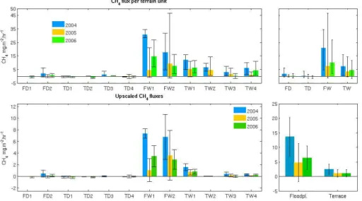
The methane fluxes show a large spatial and temporal vari-ation. The fluxes measured on the river floodplain (FW classes) are considerably higher than those of the Sphagnum-rich sites on the river terrace (TW classes). Only sites in the TW1 class show fluxes that are comparable to those of FW sites (Van Huissteden et al., 2005), although they are still lower (Fig. 11). Dry sites (TD and FD classes) generally show negative fluxes (uptake) and sometimes slightly posi-tive fluxes. Posiposi-tive fluxes decrease rapidly with lower water table (Van Huissteden et al., 2005).
Compared to van Huissteden et al. (2005), who reported about the 2004 campaign, the 2005 and 2006 field campaigns add to understanding of the temporal variation of the fluxes. Fluxes were highest in 2004, and lowest in 2005, despite the higher the air and soil temperatures. In 2006, the fluxes were intermediate, while the soil surface temperature was lower than in 2005. As such, high fluxes correspond well with high river water levels (Sect. 2.1.1). Statistical analysis shows that methane emission increases significantly with height of the water table and with active layer thickness. Methane emission decreases with surface temperature, and does not
Fig. 11. Top: Average CH4fluxes per terrain/vegetation unit. The error bars indicate the standard deviation of the average. Top right: averages for all wet and dry groups of terrace and floodplain. Bottom: upscaled fluxes by weighting of the measured fluxes by areal proportion in the terrain.
significantly vary with soil temperature at 10 cm depth. This surprising results are discussed in Sect. 5.1. The negative fluxes on dry sites do not show any significant correlation with the environmental variables above, albeit that negative fluxes only occur on sites with low water table. Sites where the water table was only a few cm below the surface may al-ready show negative methane fluxes. At water table depths below −5 cm, fluxes higher than 5 mg CH4m−2h−1do not occur and negative fluxes dominate.
Upscaling of the methane fluxes has been performed by multiplying the fluxes with the areal fraction of the different terrain units. This gives an integrated methane flux for the terrace area around the flux tower and the investigated flood-plain area (Table 5, Fig. 11). The integrated fluxes are small on the terrace compared to some of the site fluxes, due to the large relative area of dry sites (68%), which are mostly located to the east of the tower. The area to the west of the tower consists of a mosaic of dry and wet sites, associated with polygons. Particularly the polygon ridges contribute to the fraction of drier areas with negative fluxes, a phenomenon that is also known from other Siberian tundra sites (Wagner et al., 2003; Wille et al., 2007). In contrast, only 37% of the floodplain area consist of dry sites, and mosaic-like pattern are not as pronounced there. Consequently, the contribution of the floodplain sites to the integrated flux is larger consid-ering their small relative area.
4.2 Seasonal course of carbon dioxide and methane fluxes Daily fluxes of NEE, its components GPP and Reco and methane fluxes are presented in Fig. 12 for the entire period of record. The increase in GPP at the start of the growing
sea-Table 5. Up scaled methane fluxes, based on estimated areal
frac-tion of terrain types on the Terrace/tundra near the eddy correlafrac-tion tower and on the floodplain. Fluxes are given as mg CH4m−2h−1.
vegetation class 2004 2005 2006 FD1 –0.01±0.01 –±– –0.10±0.11 FD2 0.46±0.60 –0.04±0.18 –0.14±0.23 TD1 –0.10±0.16 –0.08±0.14 –0.15±0.18 TD2 –0.02±0.01 0.01±0.00 –0.18±0.06 TD3 0.06±0.09 0.001±0.001 0.02±0.003 TD4 –0.06±0.02 0.01±0.23 –0.04±0.10 FW1 7.38±0.77 1.09±1.99 3.47±1.82 FW2 6.79±3.83 3.61±4.26 2.91±1.67 TW1 1.60±0.60 0.69±0.47 0.82±0.40 TW2 0.03±0.02 0.02±0.02 –±– TW2 0.41±0.35 0.19±0.25 0.03±0.20 TW3 0.33±0.15 0.05±0.08 0.22±0.20 Floodplain 13.66±6.63 4.76±6.51 6.41±4.10 Terrace/Tundra 2.46±1.73 1.08±1.29 1.11±1.28
son of 2003 is remarkably sharp. Uptake by photosynthesis is quite variable from day to day, whereas ecosystem respira-tion rates vary much slowlier throughout the year. As a con-sequence, NEE is also quite variable, particularly in a relative sense. The growing season lasts about 60 days, in July and August. The ecosystem respiration increases steadily from the start of the growing season until the second half of Au-gust, when it starts to decline. Methane fluxes make up a significant part of the greenhouse gas budget and are largest at the onset of the growing season, when wet conditions pre-vail due to snow melt. Considering that the methane flux in
m j j a s o m j j a s o m j j a s o m j j a s o −6 −4 −2 0 2 4 6 2003 2004 2005 2006 time (month) GHG flux (g C−CO 2 e m −2 day −1 ) : NEE : R e : GPP : f CH 4 tundra : f CH 4 floodplain : f CH 4 modeled
Fig. 12. The seasonal cycles of GPP, Reco, NEE and methane flux, fCH4. The individual data points represent daily total fluxes, except for
the observed methane fluxes (data points with errorbars) which represent weekly averages. The time axis is compressed in the winter months.
carbon flux units (Table 4) is only 12% of the flux indicated in Fig. 12, the methane fluxes play only a minor role in the carbon budget.
In order to quantify inter-annual variability, daily fluxes were averaged to weekly fluxes and shown in Fig. 13. It ap-pears that interannual variability is small for ecosystem res-piration, and larger for GPP and NEE, as well as for methane fluxes. The largest variability in GPP occurs at the start of the growing season, implying that the date of snow melt and the start and length of the growing season are important factors determining the carbon and greenhouse gas balances. The variability at the end of the growing season is smaller, be-cause weather conditions are less important than the limi-tation due to the shorter day lengths. The lower panels of Fig. 13 again confirm that the greenhouse gas balance is pri-marily determined by the carbon dioxide component, with a smaller but significant role for methane fluxes. Photosynthe-sis rates are 3.5 g C m−2yr−1 in the middle of the growing season, and consistently larger in 2003.
The annually cumulative fluxes are shown in Fig. 14. These fluxes result from averaging the weekly fluxes shown in Fig. 13 over all years and then integrating. It is clear that the net carbon flux NEE is the relatively small differ-ence (−92 g C m−2yr−1) between the large terms of GPP (−232 g C m−2yr−1)and Reco (+141 g C m−2yr−1), which makes NEE sensitive to relatively small changes in ei-ther GPP or Reco. The methane emissions are 28 g C-CO2e m−2yr−1. This is equivalent to a methane emission of 4.1 g CH4m−2yr−1 and a carbon flux of 3.1 g C m−2yr−1. As a consequence, the greenhouse gas balance is negative, and the site is a net sink of −64 g C-CO2e m−2yr−1. for greenhouse gases.
The uncertainty in annual totals of NEE is typically 40 g C m−2yr−1(Goulden et al., 1996; Lee et al., 1999; Yang et al., 1999; Lafleur et al., 2001; Baldocchi, 2003). Based
on the CH4flux measurements on the terrace, the coefficient of variation of the measured fluxes is 92%; in Fig. 10 the variation of the modelled values for 5-day periods is simi-lar. Therefore we estimate the uncertainty of the methane flux measurements as 25.8 g C-CO2e m−2yr−1. Assuming that uncertainty is normally distributed, the confidence level αthat the site is a sink for carbon dioxide is α=0.94, a source for methane (α=0.22) and a sink for greenhouse gas gases (α=0.83).
Using the methodology of Frolking et al. (2007) to deter-mine the temporal evolution of radiative forcing of sustained carbon dioxide and methane fluxes, we find that on short time horizons (<13 years), the methane emission has stronger radiative impacts than the carbon dioxide sink. However, because the change in atmospheric methane concentration may be considered in equilibrium with the methane source, the radiative forcing due to methane emission has settled at 1.1×10⁻¹⁴W m−2per m2 of tundra source area, which is about 4.4×10¹²m2 in the Russian Federation and about 8.7×10¹²m2worldwide (van der Molen et al., 20071). Over time horizons longer than 13 years, the radiative effect of the sustained carbon dioxide removal from the atmosphere be-comes dominant. Considering the age of tundra is older than that, this site may be considered a sink of greenhouse gasses and acts to cool the climate.
5 Discussion
5.1 Methane fluxes
A main feature of the CH4fluxes is the very high spatial vari-ability which is related to vegetation and water table variabil-ity. The water table effect is directly related to anaerobic con-ditions in the soil and has been documented by many authors (Bartlett et al., 1992; Friborg et al., 2000; Heikinnen et al.,
−5 −4 −3 −2 −1 0 1 2 3 2003 GPP, R eco , fCH 4 (g C−CO 2 e m −2 day −1 ) R eco GPP f CH 4 2004 2005 2006 −2 −1 0 1 month NEE m j j a s o −2 −1 0 1 month GHG
Fig. 13. The interannual variability in the seasonal cycles of Reco, GPP, fCH4 (upper panel) and NEE and the net GHG balance (lower
panel). The data points represent weekly mean daily fluxes. The lower panel has the same scale as the upper panel.
m j j a s o −250 −200 −150 −100 −50 0 50 100 150 month GHG (g C−CO 2 e m −2 yr −1 ) R eco = 141 g C m −2 yr−1 GPP = −232 g C m−2 yr−1 NEE = −92 g C m−2 yr−1 f CH 4 = 28 g C m−2 yr−1 GWP = −64 g C m−2 yr−1
Fig. 14. Annually cumulative GPP, Reco, NEE and methane fluxes and the resulting GHG balance. The numbers at the right indicate the total flux in mid September, indicated by the vertical dashed line, when eddy covariance measurements were no longer available.
2002; Oberlander et al., 2002; Wagner et al., 2003; Kutzbach et al., 2004). Statistical analysis shows that the spatial het-erogeneity of the terrain mainly affects water table variation, and soil temperature to a much smaller extent. The correla-tion patterns with soil temperature and active layer thickness further confirm the dominating effect of the water table. The negative correlation of soil surface temperature and the poor correlation of soil temperature at 10 cm depth with methane emission rates seems to contradict the often reported
posi-tive effect of temperature on methane fluxes of higher soil temperatures, related to microbial reaction rates (cf. Mor-rissey and Livingston, 1992; Christensen et al., 1995, 2003; Verville et al., 1998; Treat et al., 2007). We hypothesize that this reflects the evaporative cooling effect of the wet soil sur-face, and the generally thinner active layer on the terrace. Also the adaptation of the microbial population to low tem-peratures, causing high production rates even at near-zero temperatures, contributes to the low temperature sensitivity
of the CH4fluxes (Wagner et al., 2003; Rivkina et al., 2007). Apparently, the sensitivity of CH4fluxes to temperature per-tains rather to large scale variations between sites at differ-ent latitudes (Christensen et al., 2003) than within-site and short-term temporal variation in temperature. The positive correlation of methane flux with active layer depth may be a secondary effect. High water tables increase the methane flux but flooding also tends to increase active layer thickness (French, 1996, and references therein). Also, the active layer thickness co-varies with substrate availability throughout the season (see above). The main driver of methane emission is water table, which determines soil temperature and active layer thickness as well, particularly on the river terrace.
Water table also drives the temporal variability of the CH4 fluxes. On a year-to-year time scale there appears to be no clear influence of temperature. This does not exclude that the temperature influence should operate on a seasonal time scale, but as yet our observations lack full seasonal coverage. However, Wagner et al. (2003) also report absence of any correlation of CH4fluxes with soil temperature from a site in the Lena delta. The relation of CH4 flux to water table depth is approximately exponential, the fluxes decrease very rapidly with lower water table. The river water stage appears particularly important for parts of the floodplain.
The sensitivity of the methane fluxes to water table rather than soil temperature has an important implication for cli-mate change effects on CH4fluxes from tundra landscapes. An increase of precipitation and river water discharge will have a strong influence on the methane fluxes, perhaps larger than an increase in soil temperature. In particular changes in river regime will have a comparatively large influence, since the CH4production on the floodplain is comparatively large (Van Huissteden et al., 2005). The difference between soil warming and soil wetness effects need further quantification for a better appraisal of climate change effects on methane fluxes from arctic landscapes.
5.2 Carbon dioxide fluxes
The small-scale heterogeneity that is so prominent in the methane fluxes, is much less pronounced for carbon diox-ide fluxes. Both the ecosystem respiration rates and photo-synthesis rates, measured with chambers and leaf cuvettes, were variable in time and between sites, but the amount of variation is in the order of a factor of two, and not orders of magnitude, as for methane. The variation in GPP and Reco could not be well explained by vegetation type, water table depth or active layer thickness. Moreover, soil temperature appears to determine the ecosystem respiration rates only to a limited extend (Fig. 6), as was also observed for methane. We hypothesize that small scale variations in hydrology, soil temperature, soil composition, organic matter content, active layer depth and soil moisture/water table depth are interre-lated in such a complex way that the current measurements are insufficient to untangle their individual influences.
Photosynthesis appears mainly limited by radiation (Fig. 4) and much less by temperature or vapour pressure deficit. Based on the sunhour anomalies (Sect. 2.1.1), where 2004 had significantly less and 2005 significantly more sun-hours than climatologically normal, whereas 2003 and 2006 are close to normal, the photosynthesis rates would be ex-pected to change accordingly. This is however, not the case. Instead, photosynthesis rates are largest in 2003 and rela-tively small in 2006. The explanation of this apparent incon-sistency is that the sunhour anomalies do not correlate well with the relative frequency of global radiation levels below the threshold of 200 W m−2, when photosynthesis becomes severely radiation limited (Fig. 9). Instead, the relative fre-quency of radiation limitation occurs more than average in 2003 and below average in 2006. In 2004 and 2005, this frequency is close to the mean. This implies that photo-synthesis rates indeed mainly depend on the occurrence of radiation limitation. During daytime, severe cloudiness is required to reduce global radiation levels below the thresh-old of 200 W m−2. In this perspective, the absence of large mountain ranges in northern zone of Siberian tundra may be a relevant difference with Alaska, considering the relation-ship between topography and frontogenesis that was shown for Alaska (Lynch et al., 2001). Photosynthesis rates are not often limited by temperature, except for temperatures below 4◦C. Figure 4b shows that in the temperature range between 10 and 20◦C, not much gain in maximum photosynthesis ca-pacity may be expected. Similarly, vapour pressure deficit does not often limit photosynthesis and high vapour pressure deficits are actually quite rare.
5.3 Temporal and spatial upscaling
Because our measurement setup depends on solar energy, and because of the harsh climate and the inaccessibility of the area, we were unable to measure carbon dioxide and methane fluxes in the winter period. Where previously it was thought that carbon dioxide and methane emissions from frozen soils are negligible, evidence is accumulating that they may actually make up a considerable part of the annual bal-ances. Wintertime carbon dioxide emissions may be 1.3– 10.9 g C m−2winter−1in Alaska (Fahnestock et al., (1998), 8.1 g C m−2winter−1in Greenland (Soegaard et al., 2000), 4–6 g C m−2winter−1in Vorkuta, European Russia (Heikin-nen et al., 2002). These numbers often amount to about 20% of the annual sum (Chapin et al., 2000). It should be mentioned though that due to the more continental cli-mate in Chokurdakh, the soil temperatures of ±–14◦C in
the springs of 2004, 2005 and 2006 and around ±–10◦C in 2007 (probably as a result of the deeper snow) are much colder than observed in Alaska (−5.6 to −3.6◦C, Fahnestock et al., 1998). Winter time methane emissions may be be-tween 0.2 and 0.8 g C-CH4m−2winter−1with a peak emis-sion of 7.8 g C-CH4g C m−2winter−1on wet flarks. Zimov et al. (1997) present a flux of 1.13 g C-CH4m−2winter−1
from Siberian lakes. Thus winter fluxes of carbon dioxide may be relatively small compared to the summer time NEE, but winter time methane fluxes may contribute up to an ex-tra 25% of the summer fluxes. The relative importance of methane emissions may be explained by the anaerobic con-ditions that may prevail in frozen, snow covered soils (Cor-radi et al., 2005). Also, microbial metabolism in general and production of CH4in particular, has been shown to con-tinue at subzero temperatures in arctic soils (Rivkina et al., 2000, 2007; Panikov and Sizova, 2006; Wagner et al., 2007). Assuming a winter carbon dioxide flux of 5 g C m−2yr−1 and a winter methane flux of 1 g C m−2yr−1=9 g C-CO2e m−2yr−1, would change the NEE to −87 g C m−2yr−1, the methane flux to 4.1 g C m−2yr−1 with a GWP of 37 g C-CO2e m−2yr−1, and the GHG balance from −64 to −50 g C-CO2e m−2yr−1.
In Sect. 2.1.2 it was mentioned that near 20% of the area surrounding the site consists of surface water. As the carbon dioxide exchange between lakes and the atmosphere is prob-ably smaller than between land and the atmosphere, whereas methane emissions from lakes may be larger than from dry land (Bartlett et al., 1992), the greenhouse gas balance of the larger area is probably more neutral than presented in Fig. 14. At present, information about which fraction of the larger area is covered with floodplain is lacking. Therefore we have not taken the contribution of floodplains into ac-count in the upscaling, which would cause an underestima-tion of the methane emission.
5.4 Short-term and long-term sensitivity
On the short-term, the carbon dioxide balance of this tun-dra ecosystem may be influenced by primarily photosynthe-sis rates as a function of cloud-radiation interactions and by respiration rates via temperature. Another short-term change may be through changes in the length of the growing season. All other things remaining equal, Fig. 14 suggests that longer growing seasons are in favour of a stronger carbon dioxide sink if thawing starts earlier, but in favour of a reduced sink if the end of the growing season is postponed. This difference is because respiration is limited by temperature at the start, whereas photosynthesis is limited by sunlight at the end of the season. Apart from light limitation, phenology also de-termines photosynthesis rates. Methane fluxes are most di-rectly affected by changes in the hydrological cycle (Moore et al., 1993; Walter et al., 1996).
On the longer-term, changes in climate may impact the carbon dioxide balance through changes in vegetation com-position and permafrost conditions, whereas methane fluxes depend on vegetation composition as well and on hydrology. We should be very careful to explain our observations in the perspective of climate change on the longer-term. Vegetation composition changes have been observed to occur in Alaska (Jia et al., 2003; Lloyd et al., 2003; McGuire et al., 2003; Wilmking et al., 2006) as well as for western Siberia (Esper
and Schweingruber, 2004), but similar studies in NE Siberia are lacking.
5.5 Comparison with other sites
A comparison of the carbon dioxide and methane fluxes ob-served in Chokurdakh with those obob-served at other arctic tun-dra sites is given in Table 6. The mean daily carbon diox-ide flux is within the range observed for different vegetation types in Greenland. On an annual scale, the carbon dioxide sink is quite a bit larger than observed at other sites. Some sites in Alaska and Greenland even act as sources of carbon dioxide. The smaller NEE at other sites may be explained by the smaller GPP at Vorkuta (Heikinnen et al., 2002) and the larger Recoat Toolik Lake (Oberbauer et al., 1998). The smaller NEE at Greenland (Soegaard et al., 2000) may be ex-plained by the shorter growing season there. Possibly, a gen-eral explanation of the large NEE is that the site experiences a more continental climate than other sites, so that ecosystem respiration is limited by the cold soils, with temperatures lag-ging behind the air temperatures, but with warm summers, which stimulates photosynthesis. Daily methane fluxes are variable between the sites, due to vegetation, and change sub-stantially during the season. Nevertheless, the daily methane fluxes are well in the range found in the literature, be it often on the larger side. Annual fluxes are also quite comparable between sites, with the exception of the fluxes measured in the floodplains of the Kolyma river (Corradi et al., 2005), which are much higher, probably as a result of the high water table and the high nutrient availability.
6 Conclusions
At an arctic tundra site in North East Siberia, near the village of Chokurdakh in the lowlands of the Indi-girka river, we observed an mean annual carbon diox-ide flux of −92 g C m−2yr−1, which is the net result of 232 g C m−2yr−1of uptake by photosynthesis and a release of 141 g C m−2yr−1as ecosystem respiration. The mean an-nual methane emission amounts to 28 g C-CO2e m−2yr−1 (=4.1 g CH4m−2yr−1), so that the net greenhouse gas bal-ance becomes −64 g C-CO2e m−2yr−1. Because the emitted methane is removed from the atmosphere by oxidation, the radiative effect of the sustained carbon dioxide sink domi-nate over time horizons longer than 13 years, which, consid-ering the old age of the site, means that the site acts to cool the global climate. The greenhouse gas balance would prob-ably be more neutral if winter fluxes and the percentage of lakes and floodplains would be taken into account. The net carbon dioxide flux is large compared to other arctic tundra sites, probably as a result of the more continental climate. On the short-term, photosynthesis appears to depend most on the frequency of radiation limitation due to severe cloudi-ness, ecosystem respiration rates depend on temperature, but
Table 6. Comparison of daily and annual carbon dioxide and methane fluxes measured at arctic tundra. In some occasions, hourly fluxes
were integrated to daily fluxes by multiplying with 24 h per day.
region site vegetation type remarks NEE CH4flux reference
daily annual daily annual
gC gC gC-CO2e gC-CO2e
m−2d−1 m−2yr−1 m−2d−1 m−2yr−1
Alaska Barrow wet sedge tundra – −55.5 – – Kwon et al., 2006
Alaska Barrow moist tussock tundra – +18.3 – – Kwon et al., 2006
Alaska Yuken-K. Delta wet meadow – – 0.90 – Bartlett et al., 1992
Alaska Yuken-K. Delta dry upland tundra – – 0.01 – Bartlett et al., 1992
Alaska Yuken-K. Delta large tundra lakes – – 0.02 – Bartlett et al., 1992
Alaska Yuken-K. Delta small tundra lakes – – 0.48 – Bartlett et al., 1992
Alaska Toolik Lake tussock tundra 0.32 – 0.01–0.06 – Oberbauer et al., 1998
Alaska Toolik Lake wet sedge meadow control – – 0.50 30.7 King et al., 1998
Alaska Toolik Lake wet sedge meadow moss removal – – 0.53 36.1 King et al., 1998
Alaska Toolik Lake wet sedge meadow sedge removal – – 0.04 3.8 King et al., 1998
Greenland Zackenberg Cassiope heath −0.60 – 0.00 – Christensen et al., 2000
Greenland Zackenberg hummocky fen −4.80 – 0.90 – Christensen et al., 2000
Greenland Zackenberg continous fen −2.88 – 1.35 – Christensen et al., 2000
Greenland Zackenberg grasland −4.80 – 0.41 – Christensen et al., 2000
Greenland Zackenberg salix arctica −0.60 – 0.00 – Christensen et al., 2000
Greenland Zackenberg overall −2.30 – 0.29 – Christensen et al., 2000
Greenland Zackenberg fen area July – – 0.75 23.2 Friborg et al., 2000
Greenland Zackenberg fen area Aug – – 0.06–0.09 – Friborg et al., 2000
Greenland Zackenberg integrated pre-season – 8.4 – – Soegaard et al., 2000
Greenland Zackenberg integrated growing season – −18.8 – – Soegaard et al., 2000
Greenland Zackenberg integrated winter – 8.1 – – Soegaard et al., 2000
Greenland Zackenberg integrated all year – −2.3 – – Soegaard et al., 2000
Greenland Zackenberg fen + grass all year – −18.8 – – Soegaard et al., 2000
Greenland Zackenberg heath all year – 5.2 – – Soegaard et al., 2000
Greenland Zackenberg willow all year – 0.6 – – Soegaard et al., 2000
Sweden Stordalen bogs+mires eddy covariance – – 0.46 – Christensen et al., 2004
Sweden Stordalen bogs+mires chambers – – 0.40–0.45 – Christensen et al., 2004
Eur. Russia Vorkuta tundra wetland – −29.0 – 4.9 Heikinnen et al., 2002
Eur. Russia Vorkuta tundra wetland – −34.6 0.28 – Heikinnen et al., 2004
Siberia transsect various mean – – 0.29 – Christensen et al., 1995
Siberia Lena delta Carex aquatilis depression – – 0.33 – Wagner et al., 2003
Siberia Lena delta mosses rim – – 0.03 – Wagner et al., 2004
Siberia Lena delta polygon depression 45% of area – – 0.18 – Kutzbach et al., 2004
Siberia Lena delta polygon rim 55% of area – – 0.03 – Kutzbach et al., 2004
Siberia Chokurdakh mixed moist tundra −1.53 −92 0.47 28 this study
Siberia Cherskii horsetail grassland – – 1.44 – Tsuyuzaki et al., 2001
Siberia Cherskii Carex grassland – – 0.46 – Tsuyuzaki et al., 2001
Siberia Cherskii Eriophorum grassland – – −0.01 – Tsuyuzaki et al., 2001
Siberia Cherskii tussock tundra – −38.0 – 100 Corradi et al., 2005
also on water level, active layer depth and time in the grow-ing season. Methane fluxes are highly variable on small spa-tial scales. This heterogeneity is primarily related to depth of the water table and on the occurrence of vegetation types with aerenchyma, to transport methane from the soil to the atmosphere. Further variation may be explained by the exu-dation of labile organic compounds by plant roots, which is related to photosynthesis rates, soil temperature, and active layer depth. The methane fluxes are insensitive to soil tem-perature but depend strongly on changes in hydrologic con-ditions. Potential positive feedbacks between climate change
and arctic methane fluxes are likely to be governed by pre-cipitation increase next to warming for this continuous per-mafrost area.
Acknowledgements. The investigations were supported by the
Research council for Earth and Life Sciences (ALW) with financial aid from the Netherlands Organization for Scientific Research (NWO, grant no. 854.00.018) and the Darwin Center for Biogeol-ogy of ALW/NWO and by the European Commission under the Fifth Framework Programme TCOS-Siberia (EVK2-2001-00143).