HAL Id: hal-01003853
https://hal.inria.fr/hal-01003853v4
Submitted on 5 Jul 2017
HAL is a multi-disciplinary open access
archive for the deposit and dissemination of sci-entific research documents, whether they are pub-lished or not. The documents may come from teaching and research institutions in France or
L’archive ouverte pluridisciplinaire HAL, est destinée au dépôt et à la diffusion de documents scientifiques de niveau recherche, publiés ou non, émanant des établissements d’enseignement et de recherche français ou étrangers, des laboratoires
Simulating diffusion processes in discontinuous media:
Benchmark tests
Antoine Lejay, Géraldine Pichot
To cite this version:
Antoine Lejay, Géraldine Pichot. Simulating diffusion processes in discontinuous media: Benchmark tests. Journal of Computational Physics, Elsevier, 2016, 314, pp.384 - 413. �10.1016/j.jcp.2016.03.003�. �hal-01003853v4�
Simulating Diffusion Processes
in Discontinuous Media:
Benchmark Tests
Antoine Lejay
*†‡SGéraldine Pichot
¶‖July 5, 2017
Abstract
We present several benchmark tests for Monte Carlo methods simulating diffusion in one-dimensional discontinuous media. These benchmark tests aim at studying the potential bias of the schemes and their impact on the estimation of micro- or macroscopic quantities (repartition of masses, fluxes, mean residence time, . . . ). These benchmark tests are backed by a statistical analysis to filter out the bias from the unavoidable Monte Carlo error. We apply them on four different algorithms. The results of the numerical tests give a valuable insight of the fine behavior of these schemes, as well as rules to choose between them.
Keywords. Monte Carlo methods for discontinuous media; Fick’s law; breakthrough curve
Note. This is a corrected version of the article with the same title published in Journal of Computational Physics in 2016. The correction concerns the Uffink algorithm, Eq. (25) and Eq. (23).
*Université de Lorraine, IECL, UMR 7502, Vandœuvre-lès-Nancy, F-54500, France †CNRS, IECL, UMR 7502, Vandœuvre-lès-Nancy, F-54500, France
‡Inria, Villers-lès-Nancy, F-54600, France
SContact: IECL, BP 70238, F-54506 Vandœuvre-lès-Nancy CEDEX, France. Email: [email protected]
¶Inria, Rennes, France
‖Contact: Inria de Paris, Inria, 2 rue Simone Iff, CS 42112, 75589 Paris Cedex 12, France. Email: [email protected]
1
Introduction
Many diffusion models arising in geophysics, population ecology and biology involve second-order operators of type ∇(𝐷∇·) with a discontinuous diffusivity 𝐷. Monte Carlo methods provide simple ways to solve diffusion problems. Random walk techniques are popular in the geophysical community [55, 57]. Basically, the physical quantity of interest (e.g. the concentration of a solute) is approximated by averaging a suitable function over the positions of a large cloud of particles. For this, we need a rule for moving the particles during a small (deterministic or random) time step in a way which respects the physics. For linear equations, the particles move independently. Besides, their random future positions depend only on their current ones as well as on their immediate environments.
A simple technique when 𝐷 is differentiable is to move the particle during a time step 𝛿𝑡 from its position 𝑥 to
𝑥 + 𝜉√︀2𝐷(𝑥)𝛿𝑡 +∇𝐷(𝑥)𝛿𝑡, (1) where 𝜉 follows the unit, centered normal distribution.
This scheme no longer works when 𝐷 is discontinuous (see e.g. [19, 27] for numerical tests). The latter case is still a challenging problem. However, the dynamic of the particles is now well understood for one-dimensional media.
Many interpretations and simulation techniques have been proposed during the last twenty years. Some numerical methods consider only the mathematical aspect of the simulation [12–14, 30, 31, 36–38] while others are driven by applications in a specific field: in geophysics [1–4, 9, 11, 22, 24–27, 33, 35, 43–46, 48, 55], fluid/gas dynamics [21], ecology [8, 42, 47], brain imaging [16], astrophysics [34, 56], meteorology [54], oceanography [19, 20, 53], molecular dynamics [7, 39], among others.
To validate the numerical methods, different benchmark tests have been developed. In [26, 27], several schemes are tested by comparing the concentration with analytic solutions and by checking that the proportion of particles on each side of the interface is correct in the steady state regime. In [26], the different schemes are also qualitatively evaluated for symmetry. In [52] and [19], which are related to oceanography, density and residence times are compared with respect to known values. In [4, 47], the first and second spatial moments in a two-layer aquifer system are estimated in a long time regime.
Our approach is different. While most of the benchmark tests in the literature aim at being realistic as e.g. in [47] or the Couplex test cases [6] or [4, Test scenarios S2-1, S2-2], the benchmark tests we propose here do not fulfil the same goal. Our objective is to quantify the bias of the schemes. The bias is the error induced
by the approximation schemes. The smaller, the better. However, the bias may be small in front of the Monte Carlo error. Monte Carlo simulations, justified by the law of large numbers, comes with an error in general of order O(𝑁−1/2), with 𝑁 the number of particles. In the benchmark tests proposed here, 𝑁 is very large — from 105 to 4× 10⁶ particles — so that the Monte Carlo error is small. Besides, we quantify it to detect potential bias of the schemes by using confidence intervals. For a given time step, the size of the domain is chosen small enough so as to maximize the number of passages through the interfaces. It is also chosen so as to easily test new schemes as the approximation scheme is applied only in a boundary layer around the interface of discontinuity. A test is passed if one cannot distinguish the bias from the Monte Carlo error. Otherwise the test failed. Invalidating a scheme does not means it should be ruled out. A scheme could be fair enough for computing some macroscopic parameters but not for dealing with microscopic ones.
As we are interested in the behavior of schemes taking the discontinuities of the diffusivity into account, we consider that the diffusivity is piecewise constant over the medium. We do not consider situations where the diffusivity varies regularly not to add supplementary approximation errors. Our benchmark tests concern both the transient and the steady state regime. We propose five benchmark tests: ∙ Density:
– Medium description: an infinite medium with an interface at 𝑥𝐼 = 0, and diffusivities 𝐷− at the left and 𝐷+ at the right of it.
– Test: check if the particles has the correct distribution in a bimaterial infinite medium.
∙ Layer:
– Medium description: a periodic medium [0, 𝐿] of diffusivity 𝐷0, excepted on a layer of diffusivity 𝐷𝑚 on [𝐿/2− ℓ, 𝐿/2 + ℓ].
– Test: check if the deviation from the uniform distribution is significant or not. Indeed, in the steady state regime, with periodic boundary conditions, whatever 𝐷, the particles should be uniformly distributed.
∙ Bimaterial:
– Medium description: a medium [0, 𝐿] with one interface at 𝑥𝐼 = 𝐿/2, a diffusivity 𝐷− (resp. 𝐷+) on [0, 𝑥𝐼] (resp. [𝑥𝐼, 𝐿]) and reflecting boundary conditions (BC).
– Test: check if the proportion of particles in the right-hand side of the medium is accurate, as this quantity may be analytically computed. ∙ Bimaterial absorbing I & II:
– Medium description: medium [0, 𝐿] with one interface at 𝑥𝐼 = 𝐿/2, a diffusivity 𝐷− (resp. 𝐷+) on [0, 𝑥𝐼] (resp. [𝑥𝐼, 𝐿]) and a reflecting BC at 0 and an absorbing BC at 𝐿.
– Test: check the accuracy of the loss of mass when one of the boundary is absorbing.
∙ Symmetry:
– Medium description: same medium and same BC as Bimaterial.
– Test: check whether or not the density q(𝑡, 𝑥, 𝑦), that is the density of the probability of a particle to go from 𝑥 to a small volume around 𝑦 during the time 𝑡, is symmetric in 𝑥 and 𝑦. The more the scheme respects this property of symmetry, the better.
We apply those benchmark tests on four schemes with constant time steps (our framework is not the one of Continuous Time Random Walks, which consider random time steps, see e.g. [35] and references within), namely,
∙ The exact density-based, constant time step algorithm based on the exact method proposed by [28],
∙ The algorithm based on the approximation method proposed by Uffink [55], ∙ The algorithm based on the approximation method proposed by Hoteit
et al. [22],
∙ A simpler version of the exact density-based algorithm with a linear interpo-lation for the time in case of crossing [28].
The numerical studies show the accurate or odd behavior of each schemes when computing the steady state and the transient regime.
Outline. A reminder on some theoretical results about stochastic processes are given in Section 2. Section 3 presents the five benchmark tests together with their theoretical foundations. We illustrate the use of these benchmark tests on four algorithms presented in Section 4. The results of the numerical simulations are presented in Section 5. Finally, we expose our conclusions in Section 6. Notice the two first Sections have been written so that the benchmark tests can be easily reused to test other schemes.
2
Theoretical results on diffusion processes, assumptions
and methods
We present very briefly the results regarding stochastic processes on which our benchmark tests are based. The Monte Carlo methods are built on the simulation of these processes.
2.1 Stochastic processes and Fokker-Planck equations
We consider only one-dimensional medium [0, 𝐿] of finite size with periodic, reflecting or absorbing boundary conditions (BC). The medium is defined by its diffusivity 𝐷 on [0, 𝐿] and the BC at 0 and 𝐿.
The particles are initially distributed with a probability 𝜈. At time 𝑡, they are distributed with a density 𝑓 (𝑡,·) solution to
⎧ ⎪ ⎪ ⎪ ⎪ ⎪ ⎪ ⎪ ⎪ ⎪ ⎨ ⎪ ⎪ ⎪ ⎪ ⎪ ⎪ ⎪ ⎪ ⎪ ⎩ 𝜕𝑡𝑓 (𝑡, 𝑦) =∇(𝐷(𝑦)∇𝑓(𝑡, 𝑦)), 𝑓 (𝑡,·)−−−→weakly 𝑡→0 𝜈,
𝐷(0)∇𝑓(𝑡, 0) = 𝐷(𝐿)∇𝑓(𝑡, 𝐿) = 0 for reflecting BC at 0 and 𝐿, or 𝑓 (𝑡, 0) = 𝑓 (𝑡, 𝐿) for periodic BC,
or {︃
𝐷(0)∇𝑓(𝑡, 0) = 0
𝑓 (𝑡, 𝐿) = 0 for reflecting BC at 0 and absorbing BC at 𝐿. (2) This framework can be applied to many different diffusion problems by relating the particle density to the physical quantity of interest (e.g. the concentration of a solute).
The positions of the particles are appropriately defined by the paths of a stochastic process (𝑋𝑡)𝑡≥0 indexed by the time on a probability space (Ω,ℱ, P).
The BC are taken into account in the distribution of (𝑋𝑡)𝑡≥0. For example, the particle is stopped when reaching an absorbing BC.
The process follows the Markov property. This means roughly that for a given time 𝑠 > 0, the distribution of (𝑋𝑡)𝑡≥𝑠 of the future positions depends only on 𝑋𝑠 and not on its prior positions (𝑋𝑟)𝑟<𝑠.
A numerical scheme provides us with an approximation of a path of (𝑋𝑡)𝑡≥0. Justified by the Markov property, the simplest scheme consists in simulating 𝑋𝑡+𝛿𝑡 when 𝑋𝑡 is known. This is a constant time step scheme. When 𝐷 is smooth, the process is solution to the Stochastic Differential Equations SDE [18, 41]
𝑋𝑡= 𝑥 + ∫︁ 𝑡 0 √︀ 2𝐷(𝑋𝑠) d𝑊𝑠+ ∫︁ 𝑡 0 ∇𝐷(𝑋 𝑠) d𝑠, (3)
for a Brownian motion 𝑊 . Therefore, the rule (1) with 𝑥 = 𝑋𝑡 provides such a scheme [23, 40].
If 𝐷 is discontinuous, this representation (3) is no longer valid. However, a diffusion process is associated to the divergence-form operator ∇(𝐷(𝑦)∇·). A large amount
of known results on the links between SDE and differential operators remain true, despite 𝑋 is not solution to some SDE.
For numerical approximation, knowing the density of 𝑋𝑡 given 𝑋𝑠 = 𝑥 for each 𝑡 > 𝑠 is sufficient. As the diffusivity is homogeneous in time, the densityq(𝑡−𝑠, 𝑥, 𝑦) of 𝑋𝑡 given 𝑋𝑠= 𝑥, called the fundamental solution (or Green function) of ∇(𝐷∇·) is solution to the Fokker-Planck (or Kolmogorov forward ) equation
⎧ ⎪ ⎪ ⎨ ⎪ ⎪ ⎩ 𝜕𝑡q(𝑡, 𝑥, 𝑦) = ∇𝑦(𝐷(𝑦)∇𝑦q(𝑡, 𝑥, 𝑦)), q(𝑡, 𝑥, 𝑦)−−−→weakly 𝑡→0 𝛿𝑥(𝑦),
q(𝑡, 𝑥,·) satisfies absorbing, reflecting or periodic BC. The density 𝑓 (𝑡, 𝑦) solution to (2) is then equal to
𝑓 (𝑡, 𝑦) = ∫︁ 𝐿
0
𝜈( d𝑥)q(𝑡, 𝑥, 𝑦). (4)
The probability current or flux is 𝐽 (𝑡, 𝑦) =−𝐷(𝑦)∇𝑦𝑓 (𝑡, 𝑦). For each 𝑡 > 0, 𝐽 (𝑡,·) is continuous over the medium, even in presence of discontinuities. At some point 𝑥𝐼 of discontinuity of 𝐷, 𝐽 (𝑡, 𝑥𝐼−) = 𝐽(𝑡, 𝑥𝐼+) implies that
𝐷(𝑥𝐼−)∇𝑓(𝑡, 𝑥𝐼−) = 𝐷(𝑥𝐼+)∇𝑓(𝑡, 𝑥𝐼+). (5) The proportion 𝑝[𝑎,𝑏] of particles in a box [𝑎, 𝑏] ⊂ [0, 𝐿] is 𝑝[𝑎,𝑏](𝑡) =
∫︀𝑏
𝑎𝑓 (𝑡, 𝑦) d𝑦. Integrating (2), its variation is
𝜕𝑡𝑝[𝑎,𝑏](𝑡) = 𝐽 (𝑡, 𝑎)− 𝐽(𝑡, 𝑏). (6) Hence, with 𝑁 particles at positions 𝑋𝑡(𝑖) at time 𝑡, 𝑝[𝑎,𝑏](𝑡) is easily approximated by 𝑝[𝑎,𝑏](𝑡)≈ 1 𝑁 𝑁 ∑︁ 𝑖=1 1[𝑎,𝑏](𝑋𝑡(𝑖)). (7) If the BC at 0 is the same as the BC at 𝐿, then q(𝑡, 𝑥, 𝑦) = q(𝑡, 𝑦, 𝑥) for any 𝑡 > 0 and 𝑥, 𝑦∈ [0, 𝐿]. Thus 𝑥 ↦→ q(𝑡, 𝑥, 𝑦) also satisfies (5).
2.2 Piecewise constant diffusivity
When the diffusivity is constant and equal to 𝐷 =1/2 over an infinite medium, the stochastic process 𝑋 is simply the Brownian motion and q(𝑡, 𝑥, 𝑦) is nothing more than the Gaussian kernel
g(𝑡, 𝑦− 𝑥) = √1 2𝜋𝑡exp (︂ −(𝑥− 𝑦) 2 2𝑡 )︂ .
With 𝐷(𝑥) = 𝐷+ if 𝑥≥ 0 and 𝐷− if 𝑥≤ 0, the density transition function of the process X is (see e.g. [28, 55])
q(𝑡, 𝑥, 𝑦) = 1 √︀2𝐷(𝑦)p𝜃 (︃ 𝑡, 𝑥 √︀2𝐷(𝑥), 𝑦 √︀2𝐷(𝑦) )︃ , (8) with 𝜃 = √ 𝐷+−√𝐷− √ 𝐷++√𝐷−. (9)
Herep𝜃(𝑡, 𝑥, 𝑦) is the density transition function of the Skew Brownian motion of parameter 𝜃 [29] defined by
p𝜃(𝑡, 𝑥, 𝑦) =g(𝑡, 𝑦− 𝑥) + sgn(𝑦)𝜃g(𝑡, |𝑦| + |𝑥|).
In [28], we have constructed a scheme to simulate 𝑋𝑡+𝛿𝑡 from 𝑋𝑡 by using (8). In a more general situation (finite media, presence of several discontinuities), there is no simple formula for the density transition function. Yet in short time, q(𝛿𝑡,·, ·) given by (8) could be used as an approximation of this density.
From the numerical point of view, the displacement of the particle during 𝑡 and 𝑡+𝛿𝑡 is mostly influenced by the value of 𝐷 close to 𝑋𝑡, in a region of size O(
√
𝛿𝑡). For this reason, assuming a piecewise constant diffusivity is not restrictive at all provided that √𝛿𝑡 is small enough with respect to the distance between two discontinuities (see Section 3.6 as well as [28]).
2.3 Significance tests
Denote by 𝑋𝑡 (resp. 𝑋𝑡) the position of the particles at time 𝑡 moved with the real dynamics (resp. when one of the scheme is used), and by 𝑋𝑡(𝑖) (resp. 𝑋(𝑖)𝑡 ) the position at time 𝑡 of the 𝑖-th particle moved with the real dynamics (resp. when one of the schemes is used) when 𝑁 independent particles paths are drawn. A part of our methodology relies on the theory of significance tests (see e.g. [17, Chap. 12] or [10]). To be more precise, we estimate the distance between a value Λ and an empirical quantities Λ𝑁 (resp. Λ𝑁) constructed using 𝑁 particle moving according to the true dynamics (resp. the scheme). Typically, Λ = 𝑝𝒱(𝑡) = P[𝑋𝑡 ∈ 𝒱] for a volume 𝒱. Its numerical approximation, combining the scheme and the Monte Carlo method, is Λ𝑁 = 𝑁−1#{𝑖; 𝑋
(𝑖)
𝑡 ∈ 𝒱} for 𝑁 independent realizations of the positions of the particles moving according to one of the schemes. We place ourselves in situation where thanks to the Central Limit Theorem, for 𝑁 large enough, √𝑁 (Λ𝑁 − Λ) is close in distribution to 𝜅𝐺 for a constant 𝜅 and 𝐺 is
a unit, centered normal distribution 𝒩 (0, 1). We fix a confidence level 𝛼 close to 1 and we set 𝑑𝛼 so that
P[𝐺∈ [−𝑑𝛼, 𝑑𝛼]] = 𝛼. (10) To draw a conclusion from our test, we then compare √𝑁|Λ𝑁 − Λ| with 𝜅𝑑𝛼. We use for 𝛼 = 99 %, so that 𝑑𝛼 = 2.57. When Λ(𝑡) and 𝜅(𝑡) depend on a parameter 𝑡, 𝑡↦→ ±𝜅(𝑡)𝑑𝛼 is called a confidence band.
In the several situations we consider, alternative statistical tests could be con-structed. However, for the sake of simplicity, we prefer simple procedures combined with graphical approaches.
3
Benchmark tests
A good benchmark test should be
∙ Physically relevant, i.e., relative to a quantity of practical interest.
∙ Numerically relevant, i.e. sensitive to a quality or default of the scheme to replicate a physical phenomenon, a correct flux for example.
∙ Analytically relevant, i.e. the quantity of interest may be compared with an exact or a well approximated value.
∙ Statistically relevant as using empirical means over 𝑁 particles leads to quantifiable fluctuations. This last point is important to discriminate the bias from the Monte Carlo error.
We consider five benchmark tests built on these criteria:
∙ Density: an infinite, bimaterial medium of diffusivity 𝐷− (resp. 𝐷+) on each side of the interface.
∙ Layer: a periodic medium [0, 𝐿] of diffusivity 𝐷0, excepted on a layer of diffusivity 𝐷𝑚 on [𝐿/2− ℓ, 𝐿/2 + ℓ].
∙ Bimaterial: a medium [0, 𝐿] with one interface at 𝑥𝐼 = 𝐿/2, a diffusivity 𝐷− (resp. 𝐷+) on [0, 𝑥𝐼] (resp. [𝑥𝐼, 𝐿]) and reflecting boundary conditions (BC).
∙ Bimaterial absorbing: medium [0, 𝐿] with one interface at 𝑥𝐼 = 𝐿/2, a diffusivity 𝐷− (resp. 𝐷+) on [0, 𝑥𝐼] (resp. [𝑥𝐼, 𝐿]) and a reflecting BC at 0 and an absorbing BC at 𝐿
∙ Symmetry: same conditions as Bimaterial.
3.1 Density benchmark test: check the distribution of the particles in an infinite bimaterial medium
In this benchmark test, we check if the particles has the correct distribution in a bimaterial, infinite medium. For this, we use the analytic density given by (8). We also compare the distribution functions (DF).
3.1.1 Density: Description
We consider an infinite medium with an interface at 𝑥𝐼 = 0, and diffusivities 𝐷− at the left and 𝐷+ at the right of it (see Figure 1).
D− D+
xI = 0 injection
Figure 1: Medium for the Density test.
3.1.2 Theoretical results: the Kolmogorov-Smirnov distance
Let us consider two (one-dimensional) random variables 𝑋 and 𝑌 with respective distributions functions (DF) 𝐹 and 𝐺. We expect 𝑌 to be “close” to 𝑋.
Among the possible measures of the difference between 𝑌 and 𝑋 is the Kolmogorov-Smirnov distance:
𝑑KS(𝐹, 𝐺) = sup
−∞<𝑦<+∞|𝐹 (𝑥) − 𝐺(𝑥)|.
In our situation, 𝑌 represents some variable obtained through a numerical scheme, for which we only know 𝑁 independent samples 𝑌(𝑖), 𝑖 = 1, . . . , 𝑁 . Thus, we consider the empirical DF 𝐺𝑁(𝑥) := 𝑁−1∑︀𝑁𝑖=11𝑌(𝑖)≤𝑥.
The Glivenko-Cantelli theorem states that 𝐺𝑁(𝑦)−−−→
𝑁→∞ 𝐺(𝑦) for any 𝑦 (see [17, 50]). Besides, 𝐺𝑁(𝑦) follows a binomial distribution of parameter 𝐺 and the following convergence holds for each 𝑦:
√
𝑁 (𝐺𝑁(𝑦)− 𝐺(𝑦)) law −−−→
𝑁→∞ 𝐵𝑏(𝐺(𝑦)), (11)
where 𝐵𝑏 is a Brownian bridge on [0, 1] with 𝐵𝑏(0) = 𝐵𝑏(1) = 0. For each 𝑦∈ [0, 1], 𝐵𝑏(𝑦) follows the Gaussian distribution with mean 0 and variance 𝑦(1− 𝑦). The normalized Kolmogorov-Smirnov distance 𝑀KS :=
√
𝑁 𝑑KS(𝐺𝑁, 𝐺) converges as 𝑁 becomes large to the distribution of a maximum of a Brownian bridge [15, 17, 50]. Using for the null hypothesis that a DF 𝐺 — known only through the empirical DF 𝐺𝑁 — is equal to 𝐹 , a hypothesis test is performed by using a threshold 𝑑𝛼 for a confidence level 𝛼 such that P[𝑀KS ≤ 𝑐𝛼] = 𝛼. For all reasonable levels of 𝛼, 𝑐𝛼 ≤ 3 (see the tables in [51] for tabulated values).
One advantage of this metric is that the asymptotic distribution of 𝑀KS does not depend on a particular choice of 𝐹 .
3.1.3 Density: Benchmark test definition
For the medium given above, the exact density of the positions 𝑋𝑡 of the particles with 𝑋0 = 𝑥0 isq(𝑡, 𝑥0, 𝑦) with q follows the analytic formula given by (8).
To the density is associated the distribution function 𝐹 (𝑦) := 𝐹 (𝑡, 𝑥0, 𝑦) =
∫︁ 𝑦 −∞
q(𝑡, 𝑥0, 𝑧) d𝑧 = P[𝑋𝑡 ≤ 𝑧], −∞ < 𝑧 < ∞.
Similarly, we denote by q𝑁(𝑡, 𝑥0,·) and 𝐹𝑁 := 𝐹𝑁(𝑡, 𝑥0,·) the empirical density and the empirical DF obtained by 𝑁 samples of 𝑋.
The statistics of interest is then the normalized Kolmogorov-Smirnov distance 𝑀KS := sup
−∞<𝑦<+∞ √
𝑁|𝐹𝑁(𝑡, 𝑥0, 𝑦)− 𝐹 (𝑡, 𝑥0, 𝑦)| (12) for several values of 𝑡 and 𝑥0.
Density. Plot 𝑀KS defined by (12) as a function of 𝑡 and compare it with a threshold 𝑐𝛼 of the Kolmogorov-Smirnov statistics for a confidence level 𝛼, or to the value 𝑐𝛼 = 3 which corresponds to a level of risk 1− 𝛼 ≈ 3 × 10⁻⁷. 3.2 Layer benchmark test: check the distribution of the particles in
the steady state regime
In this benchmark test, we check if the particles remain uniformly distributed after many steps in the steady state regime.
3.2.1 Layer: Description
We consider a periodic medium [0, 𝐿] of diffusivity 𝐷0, excepted on a layer of diffusivity 𝐷𝑚 on [𝐿/2− ℓ, 𝐿/2 + ℓ] (see Figure 2).
D0 Dm D0
periodic periodic
0 L
0 L/2− ` L/2 + `
Figure 2: Medium for the Layer test.
3.2.2 Theoretical results: The steady-state regime — Invariant mea-sure with periodic or reflecting BC
No mass is loss when the particle evolves on [0, 𝐿] with either periodic or reflect-ing BC. Two facts are notable in this situation.
First, the Lebesgue measure 𝐿−1d𝑥 is an invariant measure of the process: if the particles are uniformly distributed at initial time 𝑡 = 0, then they remain uniformly distributed at any time 𝑡 > 0. This case is referred to the steady state.
Second, the process is ergodic with respect to this measure. In particular, the distribution of 𝑋𝑡 converges weakly to 𝐿−1d𝑥.
We refer for example to [18] for a detailed account on these notions.
We use the notations introduced in Section 2.3. The empirical DF of 𝑋𝑡/𝐿 and 𝑋𝑡/𝐿 are, for 𝑦 ∈ [0, 1], 𝐹𝑁(𝑡, 𝑦) = 1 𝑁 𝑁 ∑︁ 𝑖=1 1𝑋(𝑖) 𝑡 ≤𝐿𝑦 and 𝐹𝑁(𝑡, 𝑦) = 1 𝑁 𝑁 ∑︁ 𝑖=1 1 𝑋(𝑖)𝑡 ≤𝐿𝑦.
The DF of 𝑋𝑡/𝐿 and 𝑋𝑡/𝐿 are, for 𝑦 ∈ [0, 1],
𝐹 (𝑡, 𝑦) = P[𝑋𝑡≤ 𝐿𝑦] = E[𝐹𝑁(𝑡, 𝑦)] and 𝐹 (𝑡, 𝑦) = P[𝑋𝑡 ≤ 𝐿𝑦] = E[𝐹𝑁(𝑡, 𝑦)]. If the scheme is bias-free, then 𝐹 (𝑡, 𝑦) = 𝐹 (𝑡, 𝑦). Yet 𝐹 (𝑡, 𝑦) is only known through its empirical approximation 𝐹𝑁(𝑡, 𝑦). From the results in Section 3.1.2, especially (11), it is expected that √𝑁 (𝐹𝑁(𝑡, 𝑦)− 𝐹 (𝑡, 𝑦)) behaves asymptotically for large
𝑁 as a Brownian bridge 𝐵𝑏(𝐹 (𝑡, 𝑦)). In particular, for 𝛼∈ (0, 1), P[︀𝐵𝑏(𝑢)∈ [−𝑑𝛼
√︀
𝑢(1− 𝑢), 𝑑𝛼√︀𝑢(1− 𝑢)]]︀ = 𝛼, 0 < 𝑢 < 1, (13) where 𝑑𝛼 is defined by (10).
3.2.3 Layer: Benchmark test definition
As the uniform distribution is an invariant measure for the process 𝑋, if the particles are initially uniformly distributed over the medium, they should remain uniformly distributed as the time evolves, whatever the number of interfaces. If 𝑋0 ∼ 𝒰(0, 𝐿), then 𝑋𝑡∼ 𝒰(0, 𝐿) so that 𝐹 (𝑡, 𝑦) = 𝑦 for any 𝑦 ∈ [0, 1].
In the steady state regime, the particles remains uniformly distributed over the medium. We then check whether or not this property is respected by the scheme. We test for 𝑡 large enough (hence after many steps) the deviation of 𝐹𝑁(𝑡,·) from 𝐹 (𝑡,·) when the 𝑁 particles are uniformly distributed at 𝑡 = 0.
The statistic of interest is 𝐾𝑁(𝑡, 𝑦) :=
√
𝑁 (𝐹𝑁(𝑡, 𝑦)− 𝐹 (𝑡, 𝑦)) = √
𝑁 (𝐹𝑁(𝑡, 𝑦)− 𝑦). (14) The null hypothesis is that the empirical DF 𝐹𝑁(𝑡, 𝑦) is a realization of 𝐹𝑁(𝑡, 𝑦) = 𝑦 for any 𝑦∈ [0, 1].
We could of course have used the Kolmogorov-Smirnov distance (see Section 3.1.2). We prefer a more graphical procedure relying on (13) and (14), and normal confi-dence intervals. With this approach, the correlations between 𝐹𝑁(𝑡, 𝑥) and 𝐹𝑁(𝑡, 𝑦) for 𝑥̸= 𝑦 are not taken into account. However, this statistical test is very simple to set up. Besides, it allows one to see where the bias of the schemes take their effect, if any, unlike the Kolmogorov-Smirnov test.
Layer. For a time 𝑡 large enough, plot 𝐾𝑁(𝑡, 𝑦) and compare it with 𝑦∈ [0, 1] ↦→ ±𝑑𝛼√︀𝑦(1 − 𝑦) for a confidence level 𝛼 with 𝑑𝛼 is defined by (10).
This benchmark test is sensitive to the capacity of the numerical scheme to preserve the symmetry condition q(𝛿𝑡, 𝑥, 𝑦) = q(𝛿𝑡, 𝑦, 𝑥) for any 𝑥, 𝑦 ∈ [0, 𝐿]. As such, it is not restricted to this particular medium, and may be applied to media containing several layers for example.
3.3 Bimaterial benchmark tests: check the proportions of particles on each side of the interface in the steady state and transient regime
The third benchmark test checks the preservation of the flux condition (5) at the interface. It is a refinement of the one proposed by E. Labolle et al. [27]. It could be adapted to more general media, for example with multiple compartments. 3.3.1 Bimaterial: Description
We consider a medium [0, 𝐿] with one interface at 𝑥𝐼 = 𝐿/2 and reflecting BC (see Figure 3). The diffusivity is 𝐷− (resp. 𝐷+) on [0, 𝑥𝐼] (resp. [𝑥𝐼, 𝐿]). The particles start from an injection point at 𝑥 with an initial mass equal to 1.
D− D+
reflecting reflecting
0 L/2 injection L
Figure 3: Medium for the Bimaterial test.
3.3.2 Theoretical results: Transient regime with reflecting boundary conditions at both endpoints
We set 𝜌 := 𝐷−/𝐷+.
There exists a family 𝜆0 = 0 < 𝜆1 ≤ 𝜆2 ≤ · · · as well as a family of functions {𝜑𝑘}𝑘=0,1,··· with 𝜑0(𝑥) = 1/
√
𝐿 such that 𝜑′𝑘(0) = 𝜑′𝑘(𝐿) = 0 and ∇(𝐷∇𝜑𝑘) = −𝜆2𝑘𝜑𝑘 and ∫︁ 𝐿 0 𝜑𝑘(𝑥)𝜑𝑗(𝑥) d𝑥 = {︃ 0 for 𝑗 ̸= 𝑘, 1 for 𝑗 = 𝑘.
The eigenvalues −𝜆2𝑘 are for any 𝑘 ≥ 1, 𝜆2𝑘= 4 𝑧 2 𝑘𝐷+ 𝐿2 with tan(𝑧𝑘) √𝜌 =− tan(︂ 𝑧√𝑘 𝜌 )︂ (15) where 𝑧0 = 0 < 𝑧1 < 𝑧2 <· · · .
The eigenfunctions are 𝜑𝑘(𝑥) = 1 𝜅𝑘 {︃ cos(︀𝛼−𝑘𝑥)︀ if 𝑥∈ [0, 𝐿/2] , 𝛾𝑘cos(︀𝛼+𝑘(𝐿− 𝑥) )︀ if 𝑥∈ [𝐿/2, 𝐿] , (16) with 𝛼±𝑘 = √𝜆𝑘 𝐷±, 𝛾𝑘= cos(𝛼−𝑘𝐿/2) cos(𝛼+𝑘𝐿/2) and 𝜅 2 𝑘 = 𝐿 4(1 + 𝛾 2 𝑘) + sin(𝛼−𝑘𝐿) 4𝛼−𝑘 + 𝛾 2 𝑘 sin(𝛼+𝑘𝐿) 4𝛼+𝑘 . For this family of eigenvalues and eigenfunctions,
q(𝑡, 𝑥, 𝑦) = 1 𝐿 + +∞ ∑︁ 𝑘=1 𝑒−𝜆2𝑘𝑡𝜑 𝑘(𝑥)𝜑𝑘(𝑦). (17)
In particular,q(𝑡, 𝑥,·) decreases exponentially fast to the uniform density over [0, 𝐿]. The value of 𝜆21 is the rate of convergence towards the steady state regime.
A tractable formula for the proportion of particles at a given time 𝑡 in a volume 𝒱 is deduced from (17) through 𝑝𝒱(𝑡) =∫︀0𝐿 d𝜈(𝑥)∫︀𝒱q(𝑡, 𝑥, 𝑦) d𝑦.
The proportion of particles on [0, 𝑥𝐼] (resp. [𝑥𝐼, 𝐿]) at time 𝑡, follows from (4) so that 𝑝−(𝑡) = 𝑝[0,𝑥𝐼](𝑡) = ∫︁ 𝑥𝐼 0 𝑓 (𝑡, 𝑦) d𝑦 = ∫︁ 𝑥𝐼 0 q(𝑡, 𝑥, 𝑦) d𝑦 resp. 𝑝+(𝑡) = 𝑝[𝑥𝐼,𝐿](𝑡) = ∫︁ 𝐿 𝑥𝐼 𝑓 (𝑡, 𝑦) d𝑦 = ∫︁ 𝐿 𝑥𝐼 q(𝑡, 𝑥, 𝑦) d𝑦.
The spectral decomposition (17) of q gives an analytic expression for the proportion of particles. In particular, after a short time, 𝑝±(𝑡) converges to1/2(since 𝑥
𝐼 = 𝐿/2) at time exponential rate −𝜆21.
With (6), a scheme which respects well the flux 𝐽 (𝑡, 𝑦±) should lead to a correct variation of 𝑝±(𝑡).
Using (7), the idea of this benchmark is then to compare the theoretical evolution of 𝑝+(𝑡) with the proportion of particles on the right-hand side of the medium. In [27], it is shown that the repartition of masses is not correct if a simple Gaussian random walk is used. In the latter case, the gradient of 𝑓 is continuous at the interface, not its flux.
𝜌 2.5 5 7.5 10 12.5 15 17.5 20 100 250 500 750 𝑧1 1.838 1.934 1.966 1.982 1.991 1.998 2.002 2.005 2.024 2.027 2.027 2.028 𝑧2 3.987 4.503 4.663 4.735 4.775 4.800 4.818 4.831 4.897 4.907 4.910 4.911 𝑧3 5.651 6.647 7.256 7.532 7.664 7.737 7.853 7.854 7.951 7.968 7.973 7.975 𝑧4 7.738 8.412 9.023 9.677 10.180 10.487 10.655 10.753 11.045 11.070 11.078 11.080
Table 1: Bimaterial — Smallest positive solution 𝑧1, . . . , 𝑧4 to (15) in function of 𝜌 = 𝐷−/𝐷+ and 𝐷−= 5, from which the eigenvalues are computed.
3.3.3 Bimaterial: Benchmark test definition
We let 𝑁 particles, starting from a fixed point, evolve in the medium with reflecting boundary conditions. We still use the notations of Section 2.3.
The statistics of interest are: 𝑃𝑁(𝑡) = 1 𝑁 𝑁 ∑︁ 𝑖=1 1 𝑋(𝑖)𝑡 ≥𝐿/2 and 𝑃𝑁(𝑡) = 1 𝑁 𝑁 ∑︁ 𝑖=1 1 𝑋(𝑖)𝑡 ≥𝐿/2. (18)
The quantity 𝑃𝑁(𝑡) (resp. 𝑃𝑁(𝑡)) is the empirical mean number of particles moved with the real (resp. approximated) dynamic staying at the right side of the interface at time 𝑡, so that 𝑃𝑁(𝑡)≈ 𝑝+(𝑡).
With the spectral decomposition (17), 𝑝+(𝑡) = ∫︁ 𝐿 𝐿/2 q(𝑡, 𝑥, 𝑦) d𝑦 = 1 2 + +∞ ∑︁ 𝑘=1 𝑐𝑘(𝑥)𝑒−𝜆2𝑘𝑡 (19) where, for 𝜑𝑘(·) given by (16),
𝑐𝑘(𝑥) = 𝜑𝑘(𝑥) ∫︁ 𝐿 𝐿/2 𝜑𝑘(𝑦) d𝑦 = 𝜑𝑘(𝑥) 𝛾𝑘 𝜅𝑘𝛼+𝑘 sin (︂ 𝛼+𝑘𝐿 2 )︂ .
The first eigenvalue is 𝜆20 = 0 (corresponding to 𝑧0 = 0) and 𝜑0 = 1/ √
𝐿. We report on Table 1 the smallest positive solutions 𝑧𝑘 to (15) with 0 < 𝑧1 ≤ 𝑧2 ≤ · · · for various ratios of 𝜌 = 𝐷−/𝐷+. The eigenvalues −𝜆2𝑘 are then easily obtained. The steady-state (or stationary) regime is reached when q(𝑡, 𝑥, 𝑦) is close to a constant function and then when 𝑐1(𝑥) exp(−𝜆21𝑡) is close to 0.
Thanks to the exponential term, a truncated version of the sum up to order 4 provides a good approximation of 𝑝+(𝑡).
For each time 𝑡, 𝑁 𝑃𝑁(𝑡) is a binomial random variable with 𝑁 trials and a probability of success 𝑝+(𝑡). Using the normal approximation,
√
𝑁 (𝑃𝑁(𝑡)− 𝑝+(𝑡)) is close to a normal distribution 𝒩 (0, 𝑝+(𝑡)(1− 𝑝+(𝑡))).
Bimaterial. For a level of confidence 𝛼 close to 1, check that for 𝑡∈ [0, 𝑇 ], √ 𝑁 (𝑃𝑁(𝑡)− 𝑝+(𝑡))∈ [−𝑑𝛼 √︀ 𝑝+(𝑡)(1− 𝑝+(𝑡)), 𝑑𝛼 √︀ 𝑝+(𝑡)(1− 𝑝+(𝑡))] with 𝑑𝛼 defined by (10).
For 𝑡 large enough, 𝑝+(𝑡) is close to 1/2, and 𝑃𝑁(𝑡) fluctuates around 1/2 with variance 1/4𝑁.
3.4 Bimaterial absorbing benchmark test: check if the first exit time is correctly estimated
3.4.1 Bimaterial absorbing: Description
We now consider a medium with two compartments [0, 𝐿/2] and [𝐿/2, 𝐿] of respec-tive diffusivities 𝐷− and 𝐷+, and a reflecting BC at 0 and an absorbing one at 𝐿 (see Figure 4). Again, we set 𝜌 = 𝐷−/𝐷+.
D− D+
reflecting absorbing
0 injection L/2 L
Figure 4: Medium for the Bimaterial absorbing test.
3.4.2 Theoretical results: Loss of mass with an absorbing boundary condition
An absorbing BC condition at 𝐿 means that the particles are removed from the medium when reaching 𝐿, leading to a loss of mass. Let 𝑋 be the stochastic process associated to ∇(𝐷∇·) in a medium with an absorbing BC.
Let 𝜏 be the random variable that gives the first time 𝑡 at which 𝑋𝑡 reaches the absorbing boundary.
If the particles are initially distributed according to the probability 𝜈, P[𝜏 ≤ 𝑡] = 1 − P[𝜏 > 𝑡] = 1 − ∫︁ 𝐿 0 d𝜈(𝑥) ∫︁ 𝐿 0 q(𝑡, 𝑥, 𝑦) d𝑦. (20) This quantity P[𝜏 > 𝑡] is the probability that the particle has not been absorbed before the time 𝑡. On the other hand, a spectral decomposition also holds for q: for the ordered eigenvalues ̃︀𝜆𝑘 and the corresponding eigenfunctions ̃︀𝜑𝑘 with ̃︀𝜑′𝑘(0) = 0 and ̃︀𝜑𝑘(𝐿) = 0, q(𝑡, 𝑥, 𝑦) = +∞ ∑︁ 𝑘=0 𝑒−̃︀𝜆2𝑘𝑡𝜑̃︀𝑘(𝑥) ̃︀𝜑𝑘(𝑦) with ∫︁ 𝐿 0 ̃︀ 𝜑𝑘(𝑥) ̃︀𝜑𝑗(𝑥) d𝑥 = {︃ 0 for 𝑗 ̸= 𝑘, 1 for 𝑗 = 𝑘. (21)
The eigenvalues −̃︀𝜆2𝑘 are given by ̃︀ 𝜆2𝑘 = 4𝑧̃︀ 2 𝑘𝐷+ 𝐿2 with tan (︂ ̃︀ 𝑧𝑘 √𝜌 )︂ = √ 1 𝜌 tan(𝑧̃︀𝑘) , (22)
where 0 <𝑧̃︀0 <𝑧̃︀1 <· · · . The corresponding eigenfunctions ̃︀𝜑𝑘 are ̃︀ 𝜑𝑘(𝑥) = 1 ̃︀ 𝜅𝑘 {︃ cos(𝛼̃︀−𝑘𝑥) if 𝑥∈ [0, 𝐿/2], ̃︀ 𝛾𝑘sin(𝛼̃︀ + 𝑘(𝐿− 𝑥)) if 𝑥∈ [𝐿/2, 𝐿], (23) with ̃︀ 𝛼±𝑘 = √𝜆̃︀𝑘 𝐷±, ̃︀𝛾𝑘 = cos(︁𝛼̃︀ − 𝑘𝐿 2 )︁ sin(︁̃︀𝛼 + 𝑘𝐿 2 )︁ , ̃︀𝜅 2 𝑘= 𝐿 4(1 +̃︀𝛾 2 𝑘) + sin(︀𝛼̃︀−𝑘𝐿)︀ 4𝛼̃︀−𝑘 −̃︀𝛾 2 𝑘 sin(︀𝛼̃︀+𝑘𝐿)︀ 4𝛼̃︀+𝑘 . All the eigenvalues have multiplicity 1 and ̃︀𝜆0 ̸= 0. The eigenfunction ̃︀𝜑0 never vanishes in (0, 𝐿). Hence q(𝑡, 𝑥, 𝑦) is exponentially fast decreasing and
P[𝜏 ≤ 𝑡] ≈ 1 −̃︀𝜅𝑒 −̃︀𝜆2 0𝑡 with ̃︀ 𝜅 = ∫︁ 𝐿 0 d𝜈(𝑥) ∫︁ 𝐿 0 ̃︀ 𝜑0(𝑥) ̃︀𝜑0(𝑦) d𝑦. (24) The DF 𝐺(𝑡) = P[𝜏 ≤ 𝑡] of 𝜏 is the proportion of particles that have left the medium before time 𝑡. This function 𝐺(𝑡) is related to breakthrough curves [57] and mean residence time [5].
3.4.3 Bimaterial absorbing I: Benchmark test definition For the particles starting from 𝑥, with (20) and (21),
𝐺(𝑡) = P[𝜏 ≤ 𝑡] = 1 − +∞ ∑︁ 𝑘=0 𝑒−̃︀𝜆2𝑘𝑡𝜑̃︀𝑘(𝑥) ∫︁ 𝐿 0 ̃︀ 𝜑𝑘(𝑦) d𝑦 (25) with ̃︀𝜑𝑘 given by (23) and
∫︁ 𝐿 0 ̃︀ 𝜑𝑘(𝑦) d𝑦 = sin (𝛼̃︀−𝐿/2) ̃︀ 𝛼− ̃︀ 𝜅𝑘 −̃︀ 𝛾𝑘 cos (𝛼̃︀+𝐿/2) ̃︀ 𝛼+ ̃︀ 𝜅𝑘 + ̃︀𝛾𝑘 ̃︀ 𝛼+ ̃︀ 𝜅𝑘 .
The values of the smallest positive roots ̃︀𝑧0, . . . ,𝑧̃︀4 of (22) are given in Table 2. We simulate for 𝑁 particles the first time 𝜏 at which they reach the boundary where an absorbing BC holds.
We denote by 𝐺𝑁 the empirical DF of the first exit time 𝜏 (see the entry boundary layer in Table 4 for the algorithm used to compute the exit time).
Bimaterial absorbing I. For a confidence level 𝛼, check if√𝑁 (𝐺𝑁(𝑡)−𝐺(𝑡)) belongs to the confidence band 𝑡 ↦→ ±𝑑𝛼√︀𝐺(𝑡)(1 − 𝐺(𝑡)) with 𝑑𝛼 defined by (10).
𝜌 2.5 5 7.5 10 12.5 15 17.5 20 100 250 500 750 ̃︀ 𝑧0 0.830 0.845 0.850 0.853 0.854 0.855 0.856 0.856 0.860 0.860 0.860 0.860 ̃︀ 𝑧1 2.951 3.204 3.283 3.321 3.343 3.357 3.368 3.375 3.416 3.422 3.424 3.424 ̃︀ 𝑧2 4.840 5.698 6.024 6.159 6.229 6.271 6.299 6.319 6.416 6.429 6.433 6.435 ̃︀ 𝑧3 6.630 7.449 8.221 8.748 9.024 9.167 9.249 9.301 9.496 9.517 9.523 9.525 ̃︀ 𝑧4 8.799 9.617 10.002 10.487 11.051 11.551 11.902 12.115 12.599 12.628 12.637 12.640
Table 2: Bimaterial absorbing — Smallest positive solutions 𝑧̃︀0, . . . ,̃︀𝑧4 to (22) in function of 𝜌 = 𝐷−/𝐷+ and 𝐷−= 5, from which the eigenvalues are computed.
3.4.4 Bimaterial absorbing II: Benchmark test definition
Some applications requires only an accurate estimation of the rate of convergence towards 0 of the survival probability 1− 𝐺(𝑡). We propose a second benchmark test which relies on estimating this rate of convergence.
With (24) (see Figure 5),
log(1− 𝐺𝑁(𝑡))≈ log(̃︀𝜅)− ̃︀𝜆20𝑡. (26) 0 10 20 30 40 0 0.05 0.1 0.15 Time Densit y of τ 0 20 40 60 80 −15 −10 −5 0 T− T+ Time log (1 − GN (t ))
Figure 5: Bimaterial absorbing II — Estimation of the exponential convergence of 1− 𝐺𝑁(𝑡) to 0.
We use as in [32] a linear least squares on 𝑡↦→ log(1 − 𝐺𝑁(𝑡)) on a window [𝑇−, 𝑇+]. The choice of 𝑇− and 𝑇+ is crucial. On the one hand, 𝑇− should be chosen large enough to avoid that exp(−̃︀𝜆20𝑡) dominates all the other terms. On the other hand, due to a rare event estimation problem, log(1− 𝐺𝑁(𝑡)) tends to oscillate for 𝑡 large enough: The Monte Carlo error, of order
√︁
𝐺𝑁(𝑡)(1− 𝐺𝑁(𝑡))/𝑁 , is much more bigger than 1− 𝐺(𝑡). Thus, 𝑇+ shall be chosen small enough to avoid the oscillations of log(1− 𝐺𝑁(𝑡)) (see Figure 5).
Bimaterial absorbing II. Estimate −̃︀𝜆20 from a linear least squares proce-dure on 𝑡∈ [𝑇−, 𝑇+]↦→ log(1−𝐺𝑁(𝑡)), where 𝐺𝑁 is the empirical distribution function of the first exit time from the domain by the absorbing boundary.
3.5 Symmetry benchmark tests: check if the density transition func-tion of the scheme is symmetric
3.5.1 Symmetry: Description
We use a bimaterial medium as in Figure 3.
3.5.2 Theoretical result: symmetry of the density
With periodic or reflecting BC at the endpoints 0 and 𝐿, the operator ∇(𝐷∇·) is self-adjoint and thenq(𝑡, 𝑥, 𝑦) = q(𝑡, 𝑦, 𝑥) for any (𝑥, 𝑦)∈ [0, 𝐿]2. This means that the probability to go from 𝑥 into a small volume d𝒱 around 𝑦 is the same as the probability to go from 𝑦 into a small volume d𝒱 around 𝑥. This property implies immediately that the Lebesgue measure is invariant measure for the dynamic. We denote by 𝑝−+ (resp. 𝑝+−) the proportion of particles during [0, 𝑡] that goes from the compartment at the left (𝑥≤ 𝐿/2) (resp. right) to the compartment at the right (𝑥≥ 𝐿/2) (resp. left) of the discontinuity. If the particles are uniformly distributed on each compartment, then
𝑝−+ = 2 𝐿 ∫︁ 𝐿/2 0 d𝑥 ∫︁ 𝐿 𝐿/2 d𝑦q(𝑡, 𝑥, 𝑦) = 2 𝐿 ∫︁ 𝐿 𝐿/2 d𝑥 ∫︁ 𝐿/2 0 d𝑦q(𝑡, 𝑥, 𝑦) = 𝑝+−. The symmetry property of q(𝑡, 𝑥, 𝑦) guarantees the correct exchange of particles between each compartment and the global equilibrium. Therefore, the more the scheme respects the symmetry of the density transition function, the better. 3.5.3 Symmetry: Benchmark test definition
For a box 𝑉 of small size located around 𝑦, and a particle starting at 𝑥, P𝑥[𝑋𝑡∈ 𝑉 ] =
∫︁
𝑉
q(𝑡, 𝑥, 𝑦) d𝑦 ≈ |𝑉 | × q(𝑡, 𝑥, 𝑦).
We fix some integer 𝑛 and we set 𝑥𝑖 = 𝑖𝐿/𝑛 for 𝑖 = 0, . . . , 𝑛, as well as 𝑥𝑖+1/2 the mid-point of [𝑥𝑖, 𝑥𝑖+1].
The domain [0, 𝐿] is cut into small intervals [𝑥𝑖, 𝑥𝑖+1], 𝑖 = 0, . . . , 𝑛 − 1. For 𝑁 particles 𝑋(1), . . . , 𝑋(𝑁 ), set for 𝑖, 𝑗 = 0, . . . , 𝑛,
𝑄𝑖𝑗(𝑡) = 𝑛 𝐿
#{𝑘 such that 𝑋𝑡(𝑘) ∈ [𝑥𝑗, 𝑥𝑗+1] when 𝑋0 = 𝑥𝑖+1/2} 𝑁 ≈ 𝑛 𝐿 ∫︁ (𝑗+1)𝐿/𝑛 𝑗𝐿/𝑛 q(𝑡, 𝑥𝑖+1/2, 𝑦) d𝑦 ≈ q(𝑡, 𝑥𝑖+1/2, 𝑥𝑗+1/2). (27) Thus, (𝑄𝑖𝑗(𝑡))𝑖,𝑗=0,...,𝑛−1 is a discrete approximation of the density q(𝑡,·, ·) at time 𝑡.
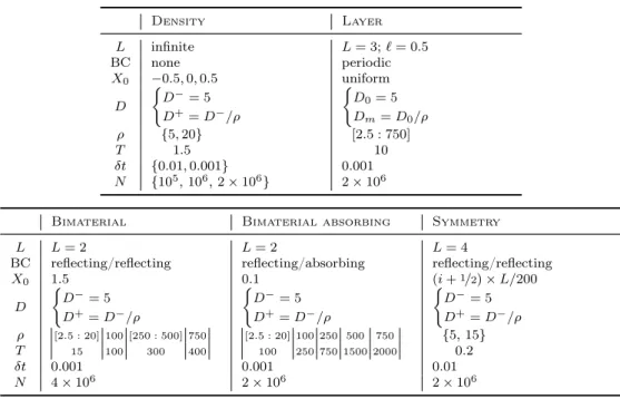
Density Layer 𝐿 infinite 𝐿 = 3; ℓ = 0.5 BC none periodic 𝑋0 −0.5, 0, 0.5 uniform 𝐷 {︃ 𝐷−= 5 𝐷+= 𝐷−/𝜌 {︃ 𝐷0= 5 𝐷𝑚= 𝐷0/𝜌 𝜌 𝑇 {5, 20} 1.5 [2.5 : 750] 10 𝛿𝑡 {0.01, 0.001} 0.001 𝑁 {105, 106, 2 × 10⁶} 2× 10⁶
Bimaterial Bimaterial absorbing Symmetry
𝐿 𝐿 = 2 𝐿 = 2 𝐿 = 4
BC reflecting/reflecting reflecting/absorbing reflecting/reflecting
𝑋0 1.5 0.1 (𝑖 +1/2)× 𝐿/200 𝐷 {︃ 𝐷−= 5 𝐷+= 𝐷−/𝜌 {︃ 𝐷−= 5 𝐷+= 𝐷−/𝜌 {︃ 𝐷−= 5 𝐷+= 𝐷−/𝜌 𝜌 𝑇 [2.5 : 20] 100 [250 : 500] 750 15 100 300 400 [2.5 : 20] 100 250 500 750 100 250 750 1500 2000 {5, 15} 0.2 𝛿𝑡 0.001 0.001 0.01 𝑁 4× 10⁶ 2× 10⁶ 2× 10⁶
Table 3: Parameters for the benchmark tests.
Symmetry. Plot the absolute value of difference ∆𝑖𝑗(𝑡) = |𝑄𝑖𝑗(𝑡)− 𝑄𝑗𝑖(𝑡)| as function of 𝑖, 𝑗 = 0, . . . , 𝑛− 1.
The matrix (∆𝑖𝑗(𝑡))𝑖,𝑗=0,...,𝑛−1measures of how much numerically the densityq(𝑡, 𝑥, 𝑦) of the scheme deviates from being symmetric in 𝑥 and 𝑦. We call it the asymmetry measure. By doing so, we refine the test proposed in [26, Sect. 4.3.3].
Here, we do not quantify the statistical fluctuations of 𝑄𝑖𝑗(𝑡), but it appears in our numerical results that it is not crucial as for the other benchmark tests.
3.6 Parameter settings: number of particles, time step and size of the domain
The parameters we use are given in Table 3. We set 𝜌 = 𝐷−/𝐷+. 3.6.1 Number of particles
We simulate the dynamic of 𝑁 particles until the final time 𝑇 is reached.
We choose a large number of particles so that the Monte Carlo error is small. Typically, Monte Carlo simulations comes with an error in general of order O(𝑁−1/2), with 𝑁 the number of particles. In the numerical simulations, we choose from 105 to 4× 10⁶ particles, so that the Monte Carlo error ranges from the order 3.2× 10⁻³ to 5× 10⁻⁴.
3.6.2 Time step and size of the domain
The time step and the size of the domain are closely linked.
For a given time step. Assume we fix the time step 𝛿𝑡 as a given input. This time step determines the size of the domain so as to maximize the number of passage through the interface layer by maximizing the relative size of the interface layer within the medium.
Indeed, increasing the size of the domain without changing the time step hides artificially the potential bias of the scheme which appears only when the particle is in the interface layer.
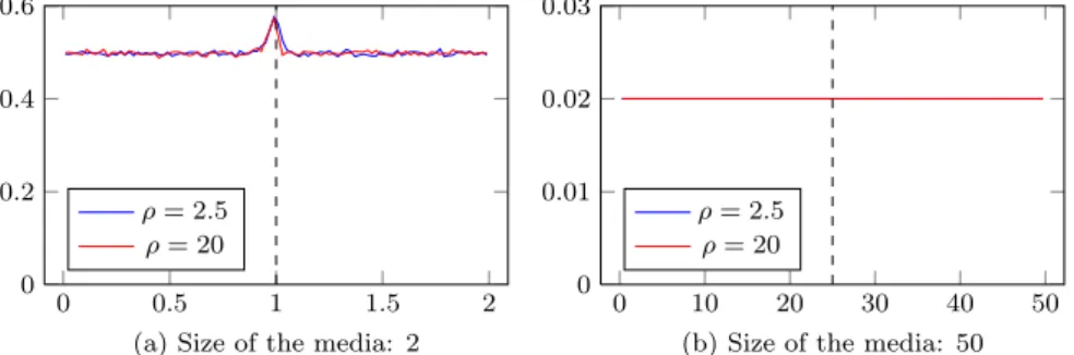
As illustration, we plot in Figure 6 the distribution of 2× 10⁶ particles in the steady state regime at time 𝑇 = 10 with a scheme used in the interface layer called SBMlin (see Algorithm 5 in Section 4 for more details). What is plotted is really an empirical estimation of the density of 𝑋𝑡 at time 𝑇 = 10 (𝛿𝑡 = 0.001), with an initial uniform distribution in a bimaterial medium with 𝐷−= 5 and 𝐷−/𝐷+= 𝜌 and reflecting BC. In Figure 6(a), for a domain size of 2 and a time step 𝛿𝑡 = 0.001, the bias of the scheme is visible around the interface. In Figure 6(b), for a domain size of 50 and the same time step 𝛿𝑡 = 0.001, the bias of the scheme is not visible.
0 0.5 1 1.5 2
0 0.2 0.4 0.6
(a) Size of the media: 2 ρ = 2.5 ρ = 20 0 10 20 30 40 50 0 0.01 0.02 0.03
(b) Size of the media: 50 ρ = 2.5
ρ = 20
Figure 6: Influence of the size of the domain for a given time step 𝛿𝑡 = 0.001: empirical estimation of the density of 𝑋𝑡. Example with a bimaterial medium in the steady state regime at time 𝑇 = 10 and the algorithm SBMlin (see Algorithm 5 in Section 4 below) in the interface layer.
For a given domain size. Assume we fix the size of the domain size as a given input. The time step must be chosen so as to keep a large amount of particles that cross the interface layer.
A caution must be observed if the time step is decreased while leaving the medium unchanged.
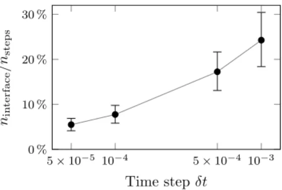
We report in Figure 7, the mean proportion of the number of steps done in the interface layer 𝑛interface over the total number of steps 𝑛steps in a fixed, bimaterial
medium. This proportion decreases quickly with the time step 𝛿𝑡. If one choose another time step, the size of the domain should be resized accordingly.
10−3 5× 10⁻⁴ 10−4 5× 10⁻⁵ 0 % 10 % 20 % 30 % Time step δt nin terface /n steps
Figure 7: Influence of the time step for a given domain size 𝐿 = 2: Mean proportion of steps performed in the interface layer as a function of the time step. Example with a bimaterial medium with 𝐷− = 5, 𝐷+ = 0.25 (𝜌 = 20) for the algorithm sbm (see Algorithm 5 in Section 4 below), 𝐿 = 2 and one interface at 𝑥𝐼 = 1, as well as reflections at both ends. The final time is 𝑇 = 10 and the 𝑁 = 10 000 particles are uniformly distributed at 𝑡 = 0. The error bars represents the limits of the 1st and 3rd quartiles.
Finally, let us mention that the mean proportion of steps in the interface layer varies from 32 % for 𝜌 = 2.5 to 25 % for 𝜌 = 750. This slight variation could contribute to the differences in the behavior of the schemes observed as 𝜌 increases. Therefore, a good benchmark test dedicated to emphasize the bias of schemes must have a domain size and a time step chosen accordingly so as to maximize the number of crossing of the interfaces.
3.6.3 Size of the domain with respect to the boundary layers
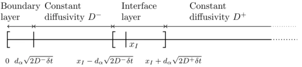
In the benchmark tests, the size of the domain is also chosen so that we can change the tested schemes and the boundary conditions independently. To do so, the domain is large enough so that a particle close to a boundary does not “see” the discontinuity and a particle close to the discontinuity region does not “see” the boundaries.
To do so, the domain is split in three kinds of zones (see Figure 8): ∙ The interface layer 𝐼layer, around a discontinuity at 𝑥𝐼,
∙ The boundary layer,
Boundary layer Interface layer Constant diffusivity D− Constant diffusivity D+ 0 dα√2D−δt xI− dα √ 2D−δt xI+ dα √ 2D+δt xI
Figure 8: Three kind of zones: interface layer, boundary layer, zone of constant diffusivity.
The size of the domain is chosen so that the interfaces and boundary layers fill most of the size of the domain without overlapping.
For a fixed the time step 𝛿𝑡 and a discontinuity at the position 𝑥𝐼, we define a zone around the interface, called the interface layer, as:
𝐼layer(𝑥𝐼) = [𝑥𝐼− 𝑑𝛼 √
2𝐷−𝛿𝑡, 𝑥𝐼+ 𝑑𝛼√2𝐷+𝛿𝑡],
with P[|𝐺| ≤ 𝑑𝛼] = 𝛼 for 𝐺 ∼ 𝒩 (0, 1). We choose 𝑑𝛼 = 4, corresponding to 𝛼 = 1− 6 × 10−5 = 99.994 %. This means that, when a particle is at a distance greater than 𝑑𝛼√2𝐷±𝛿𝑡 from the discontinuity, it has a very small probability (0.006 %) to reach it.
Identically, the particle is within a so-called boundary layer if it is at the distance lower than 𝑑𝛼
√
2𝐷±𝛿𝑡 from it.
This means that, when a particle is at distance greater than 𝑑𝛼 √
2𝐷±𝛿𝑡 from an interface or a boundary, we act as if the diffusivity is constant which defines the zones of constant diffusivity.
3.7 Algorithms
The particles are moved with a constant time step 𝛿𝑡, with an algorithm which is function of the zones defined above.
3.7.1 Algorithms in the constant diffusivity zone
In the zone of constant diffusivity, we use Gaussian (see Algorithm 1) or Uniform steps (see Algorithm 2).
3.7.2 Algorithms in the boundary layer
In the boundary layer, the hitting time may be computed either exactly (see Algorithm 3: ExactHittingTime) or with a linear approximation (see Algorithm 4: LinearHittingTimeUS and LinearHittingTimeGS).
Data: The position 𝑥 of the particle at time 𝑡, a time step 𝛿𝑡 and a diffusivity 𝐷. Result: The position 𝑋𝑡+𝛿𝑡at time 𝑡 + 𝛿𝑡 of the particle.
Draw a random variate 𝜉 ∼ 𝒩 (0, 1); return𝑥 +√2𝐷𝛿𝑡𝜉;
Algorithm 1: GaussianStep(𝑥, 𝛿𝑡, 𝐷): Gaussian step in a zone of constant diffusivity 𝐷.
Data: The position 𝑥 at time 𝑡 of the particle, a time step 𝛿𝑡 and a diffusivity 𝐷. Result: The position 𝑋𝑡+𝛿𝑡at time 𝑡 + 𝛿𝑡 of the particle.
Draw a random variate 𝑈 ∼ 𝒰(0, 1); return𝑥 +√6𝐷𝛿𝑡(2𝑈 − 1);
Algorithm 2: UniformStep(𝑥, 𝛿𝑡, 𝐷): Uniform step in a zone of constant diffusivity 𝐷.
Data: The position 𝑥 at time 𝑡 of the particle, a time step 𝛿𝑡 and a diffusivity 𝐷. Result: The position (𝑠, 𝑋𝑠)which is either (𝜏, 0) if 𝜏 < 𝑡 + 𝛿𝑡 or (𝑡 + 𝛿𝑡, 𝑋𝑡+𝛿𝑡), where
𝜏 = inf{𝑠 > 𝑡; 𝑋𝑠= 0}. Draw a random variate 𝜉 ∼ 𝒩 (0, 1);
Set 𝑧 ← 𝑥/√2𝐷 ; /* Normalize the position */
Set 𝑦 ← 𝑧 +√𝛿𝑡𝜉; /* Try a first guess */
if sgn(𝑧)̸= sgn(𝑦) then
/* The boundary/interface has been crossed. */
Generate a random variate 𝜉 ∼ ℐ𝒢(|𝑧|/|𝑦|, 𝑧2/𝛿𝑡); Set 𝜏 ← 𝛿𝑡 × 𝜉/(1 + 𝜉) + 𝑡;
return(𝜏, 0); else
/* Check if the boundary/interface has been crossed. */
Generate a random variate 𝜉 ∼ ℐ𝒢(|𝑧|/|𝑦|, 𝑧2/𝛿𝑡); Generate a random variate 𝑈 ∼ 𝒰(0, 1);
if 𝑈 < exp(−2𝑧𝑦/𝛿𝑡) then
/* The boundary/interface has been crossed. */
Generate a random variate 𝜉 ∼ ℐ𝒢(|𝑧|/|𝑦|, 𝑧2/𝛿𝑡); Set 𝜏 ← 𝛿𝑡 × 𝜉/(1 + 𝜉) + 𝑡;
return(𝜏, 0); else
/* The boundary/interface has not been crossed. */
return(𝑡 + 𝛿𝑡, 𝑦√2𝐷); end
end
Algorithm 3: ExactHittingTime(𝑡, 𝑥, 𝛿𝑡, 𝐷): Exact simulation of the first hitting time of 0, where ℐ𝒢(𝛼, 𝛽) is the inverse Gaussian distribution of parameters (𝛼, 𝛽) (see e.g. [28]).
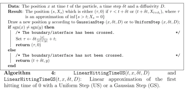
Data: The position 𝑥 at time 𝑡 of the particle, a time step 𝛿𝑡 and a diffusivity 𝐷. Result: The position (𝑠, 𝑋𝑠)which is either (𝜏, 0) if 𝜏 < 𝑡 + 𝛿𝑡 or (𝑡 + 𝛿𝑡, 𝑋𝑡+𝛿𝑡), where 𝜏
is an approximation of inf{𝑠 > 𝑡; 𝑋𝑠= 0}
Draw a new position 𝑦 according to GaussianStep (𝑥, 𝛿𝑡, 𝐷) or to UniformStep (𝑥, 𝛿𝑡, 𝐷); if sgn(𝑥)̸= sgn(𝑦) then
/* The boundary/interface has been crossed. */
Set 𝜏 ← 𝛿𝑡 |𝑥| |𝑥|+|𝑦|+ 𝑡; return(𝜏, 0)
else
/* The boundary/interface has not been crossed. */
return(𝑡 + 𝛿𝑡, 𝑦) end
Algorithm 4: LinearHittingTimeUS(𝑡, 𝑥, 𝛿𝑡, 𝐷) and LinearHittingTimeGS(𝑡, 𝑥, 𝛿𝑡, 𝐷): Linear approximation of the first hitting time of 0 with a Uniform Step (US) or a Gaussian Step (GS).
3.7.3 Algorithms in the interface layer
In the interface layer 𝐼layer(𝑥𝐼), around each interface with position 𝑥𝐼, comes into play the approximation method for which we would like to estimate the bias. 3.7.4 Summary of the possible algorithms in the different zones
For each particle, we generate a random sequence{𝑋𝑘𝛿𝑡}𝑘=0,1,2,... of approximations of {𝑋𝑘𝛿𝑡}𝑘=0,1,2,.... For this, 𝑋𝑘𝛿𝑡 depends only on 𝑋(𝑘−1)𝛿𝑡 according to a density q(𝛿𝑡, 𝑋(𝑘−1)𝛿𝑡,·), where q is an approximation of q.
Table 4 summarizes the possible algorithms according to the zone (interface layer, boundary layer, zone of constant diffusivity (see Figure 8) in which the particle is).
∙ Interface layer: scheme that has to be tested ∙ Boundary layer
⋆ absorbing: either ExactHittingTime (Algorithm 3) or LinearHittingTimeUS (Algorithm 4).
⋆ periodic: reinject the particle into the medium in a periodic way. ⋆ reflecting: perform a reflection around the boundary point.
∙ Zone of constant diffusivities: either GaussianStep (see Algorithm 1) or UniformStep (see Algorithm 2).
Table 4: Possible algorithms for the three kinds of zone.
results. A general rule is to not mix Gaussian-like steps with uniform steps. An illustration is provided in Section 4.2.
4
Four numerical schemes in one dimensional discontinuous
media
4.1 Algorithms
In the interface layer 𝐼layer(𝑥𝐼), we consider four specific schemes:
∙ SBM: The exact density based, constant time step algorithm based on the exact method proposed by [28] (We warn that a normalization factor 1/2 has been added for convenience in this reference in front of the diffusivity coefficient), see Algorithm 5.
∙ Uffink: The algorithm based on the approximation method proposed by Uffink [55], see Algorithm 6.
∙ HMYLA: The algorithm based on the approximation method proposed by Hoteit et al. [22], see Algorithm 7.
∙ SBMlin: A simpler version of the exact algorithm, with a linear interpolation for the time in case of crossing [28], see Algorithm 5.
Data: An initial position 𝑋𝑡= 𝑥and a time 𝛿𝑡 > 0 in the interface layer 𝐼layer(𝑥𝐼)of an interface at 𝑥𝐼.
Result: A position of 𝑋𝑡+𝛿𝑡 according to the SBM algorithm. (SBM) Set (𝑠, 𝑦) ← ExactHittingTime (𝑡, 𝑥 − 𝑥𝐼, 𝛿𝑡, 𝐷sgn(𝑥−𝑥𝐼)) (SBMlin) Set (𝑠, 𝑦) ← LinearHittingTimeGS (𝑡, 𝑥 − 𝑥𝐼, 𝛿𝑡, 𝐷sgn(𝑥−𝑥𝐼)) if 𝑠 < 𝑡 + 𝛿𝑡 then
/* A crossing occurred: biased step */
Generate a random variate 𝑈 ∈∼ 𝒰(0, 1); Generate a random variate 𝐺2∼ 𝒩 (0, 1); if 𝑈 < (1 + 𝜃)/2 then return𝑥𝐼 +√︀2𝐷+(𝑡 + 𝛿𝑡− 𝑠)|𝐺2| else return𝑥𝐼 −√︀2𝐷−(𝑡 + 𝛿𝑡− 𝑠)|𝐺2| end else /* No crossing occurred */ return𝑥𝐼+ 𝑦 end
Algorithm 5: SBM and SBMlin algorithms with the two-steps method.
From now, each method is associated to a color using the correspondence given in Table 5.
Data: An initial position 𝑋𝑡= 𝑥and a time step 𝛿𝑡 > 0 in the interface layer 𝐼layer(𝑥𝐼)of an interface at 𝑥𝐼
Result: A position 𝑋𝑡+𝛿𝑡 according to Uffink’s algorithm Compute 𝐻1=
√
𝐷−6 𝛿𝑡and 𝐻2=√𝐷+6 𝛿𝑡;
Set 𝑧 ← 𝑥 − 𝑥𝐼 ; /* Shift the position */
if 𝑧 + 𝐻1< 0 then
/* the interface is not crossed: uniform step */
Generate a random variate 𝑉 ∼ 𝒰(0, 1); return𝑥 + (2𝑉 − 1)𝐻1
else
if 𝑧 < 0 then
/* The interface is crossed: compute 𝑃𝐻 */
Compute 𝑥𝐿 = 𝑧− 𝐻1, 𝑥𝑀 =−𝑧 − 𝐻1 and 𝑥𝑅= (𝑧 + 𝐻1) 𝐻2 𝐻1; Compute 𝑃𝐻 = 1 2 𝐻1 (𝑥𝑀− 𝑥𝐿); else if 𝑧− 𝐻2> 0 then
/* the interface is not crossed: uniform step */
Generate a random variate 𝑉 ∼ 𝒰(0, 1); return𝑥 + (2𝑉 − 1)𝐻2
else
/* The interface is crossed: compute 𝑃𝐻 */
Compute 𝑥𝐿= (𝑧− 𝐻2) 𝐻1 𝐻2, 𝑥𝑀 =−𝑧 + 𝐻2 and 𝑥𝑅= 𝑧 + 𝐻2; Compute 𝑃𝐻 =(1 + 𝜃) 2 𝐻2
(𝑥𝑀 − 𝑥𝐿)with 𝜃 given by Eq. (9); end
end end
/* The interface is crossed: biased step */
Generate a random variate 𝑈 ∼ 𝒰(0, 1); Generate a random variate 𝑉 ∼ 𝒰(0, 1); if 𝑈 ≤ 𝑃𝐻 then
return𝑥𝐼+ 𝑥𝐿+ (𝑥𝑀− 𝑥𝐿) 𝑉 else
return𝑥𝐼+ 𝑥𝑀 + (𝑥𝑅− 𝑥𝑀) 𝑉 end
Data: An initial position 𝑋𝑡= 𝑥and a time 𝛿𝑡 > 0 in the interface layer 𝐼layer(𝑥𝐼)of an interface at 𝑥𝐼.
Result: A position 𝑋𝑡+𝛿𝑡 according to HMYLA algorithm Compute 𝐻1=
√
𝐷−6 𝛿𝑡and 𝑈2=√𝐷+6 𝛿𝑡;
Set 𝑧 ← 𝑥 − 𝑥𝐼 ; /* Shift the position */
Set (𝑠, 𝑧next)← LinearHittingTimeUS (𝑡, 𝑧, 𝛿𝑡, 𝐷sgn(𝑧)); if 𝑠 < 𝑡 + 𝛿𝑡 then
/* The interface is crossed: biased step */
/* Time splitting */
Compute 𝛿𝑡2= 𝛿𝑡− 𝑠 ;
Generate a random variate 𝑈 ∼ 𝒰(0, 1); if 𝑈 <1− 𝜃 2 then Compute 𝑥𝐿 = 𝑥𝐼−√𝐷−6 𝛿𝑡2; Set 𝑥𝑅= 𝑥𝐼; else Set 𝑥𝐿 = 𝑥𝐼; Compute 𝑥𝑅= 𝑥𝐼+√𝐷+6 𝛿𝑡2; end
Generate a random variate 𝑊 ∼ 𝒰(0, 1); return𝑥𝐿+ (𝑥𝑅− 𝑥𝐿) 𝑊;
else
/* The interface is not crossed: uniform step */
return𝑥𝐼+ 𝑧next end
SBM Green HMYLA Coral
Uffink Blue SBMlin Red Table 5: Color convention for the schemes.
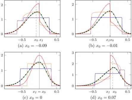
Figure 9 presents the empirical density q𝑁(𝛿𝑡, 𝑥,·) of the schemes after one step 𝛿𝑡 = 0.01 of 𝑁 = 107 particles for three values of the starting point 𝑥0 in a medium with a diffusivity 𝐷−= 5 on [−2, 0] and 𝐷+ = 0.5 on (0, 2] and reflecting boundary conditions (such a medium is referred as a bimaterial one, see Section 3.3). It illustrates the effect of the interface layer on the density depending on the starting point. −0.5 0.5 0 1 2 xI x0 (a) x0=−0.09 −0.5 0.5 0 1 2 xIx0 (b) x0=−0.01 −0.5 0.5 0 1 2 xI= x0 (c) x0= 0 −0.5 0.5 0 1 2 3 xI x0 (d) x0= 0.07
Figure 9: After one time step for different starting points. Densityq(𝑡, 𝑥0,·) (black dots) and empirical densities q𝑁(𝑡, 𝑥0,·) in an infinite bimaterial medium with 𝐷− = 5, 𝐷+ = 2 (𝜌 = 2.5) and an interface at 𝑥𝐼 = 0. We use different starting points 𝑥0 close to 𝑥𝐼. The time step is 𝛿𝑡 = 0.01. We used 𝑁 = 107 particles. The colors of the lines follows the convention of Table 5. This graphs shows how the shape of the empirical densities may vary greatly with a starting point close to the interface.
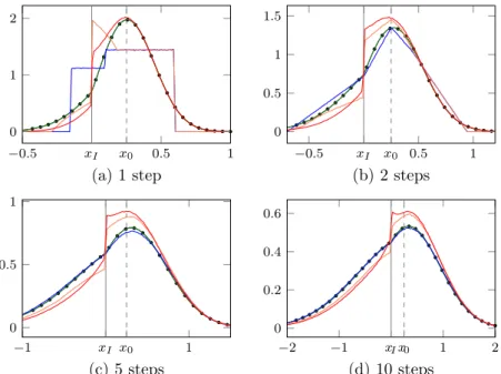
In Figure 10, we plot the empirical densities of the four methods after 1, 2, 5 and 10 time steps for a starting point 𝑥0 = 0.25, 𝑁 = 107 particles, and a discontinuity at 0. We compare it with the exact density q(𝑡, 𝑥0, 𝑦) with q given by (8). We see that empirical densities of SBMlin and HMYLA have the same behavior near the
discontinuity, while SBM — as well as Uffink after a few time steps —, follows the right dynamic. −0.5 0.5 1 0 1 2 xI x0 (a) 1 step −0.5 0.5 1 0 0.5 1 1.5 xI x0 (b) 2 steps −1 1 0 0.5 1 xI x0 (c) 5 steps −2 −1 1 2 0 0.2 0.4 0.6 xIx0 (d) 10 steps
Figure 10: After a few time steps. Density q(𝑡, 𝑥0,·) (black dots) and empirical densities q𝑁(𝑡, 𝑥0,·) in an infinite bimaterial medium with 𝐷− = 5, 𝐷+ = 2 (𝜌 = 2.5) and an interface at 𝑥𝐼 = 0. The starting point at 𝑥0 = 0.25 and the time step 𝛿𝑡 = 0.01. We used 𝑁 = 107 particles. The colors of the lines follows the convention of Table 5.
4.2 Combination of algorithms in the whole domain
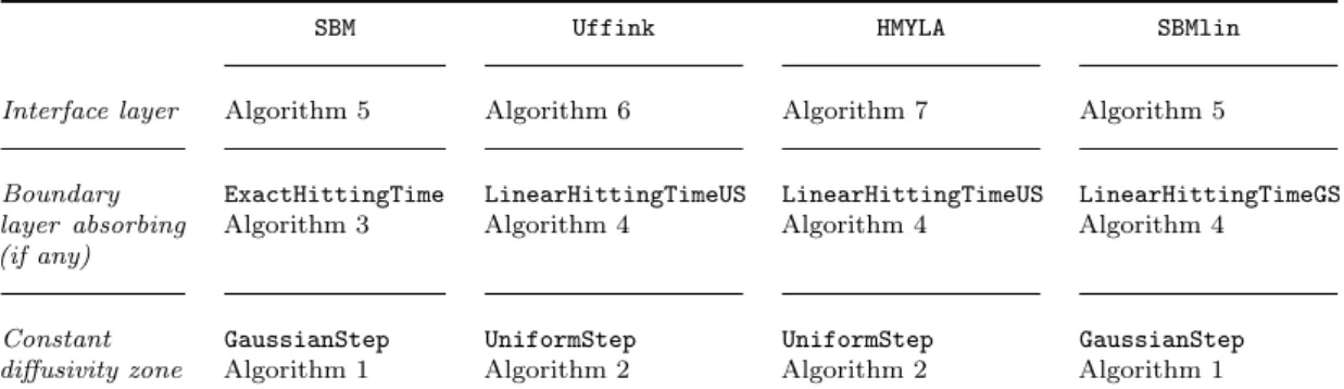
Table 6 summarizes, for each algorithm tested in the interface layer, the recom-mended combination with the algorithms proposed in Table 4 of Section 3.7.4 (see Figure 8).
Other choices could have been performed. However, this leads to bad results. In Figure 11, we show the effect of mixing the HMYLA scheme in the interface layer with the GaussianStep outside the interface layer in a bimaterial medium. With a uniform repartition of the particles and reflected boundary conditions at 0 and 2, the particle shall remain uniformly distributed all over the medium. This is not the case around the limits of the interface layers. Similar results occurs with other ways of mixing the schemes.
SBM Uffink HMYLA SBMlin
Interface layer Algorithm 5 Algorithm 6 Algorithm 7 Algorithm 5
Boundary layer absorbing (if any) ExactHittingTime Algorithm 3 LinearHittingTimeUS Algorithm 4 LinearHittingTimeUS Algorithm 4 LinearHittingTimeGS Algorithm 4 Constant diffusivity zone GaussianStep
Algorithm 1 UniformStepAlgorithm 2 UniformStepAlgorithm 2 GaussianStepAlgorithm 1 Table 6: Combination of the algorithms for the three kinds of zone.
with schemes relying on uniform approximations to avoid bad behavior when the particle is moved from one zone to another.
0 0.5 1 1.5 2 0 0.2 0.4 0.6 ρ = 2.5 ρ = 10 ρ = 20
Figure 11: Histograms of the positions of 2× 10⁶ particles at time 𝑇 = 10 (𝛿𝑡 = 0.001) in a bimaterial medium with reflected BC for HMYLA coupled with GaussianStep outside the interface layer. The dotted lines represent the limits of the interface layers for three values of 𝜌, while the dashed line represents the interface.
5
Numerical results
In this section, we apply the benchmark tests described in Section 3 to the four schemes SBM, Uffink, HMYLA and SBMlin described the Section 4. We draw conclu-sions on the behavior of each method in the steady state and transient regime. Unless stated, we use the parameters given in Table 3.
-5 x0= xI 5 0
0.1 0.2
(a) Densities qN and q
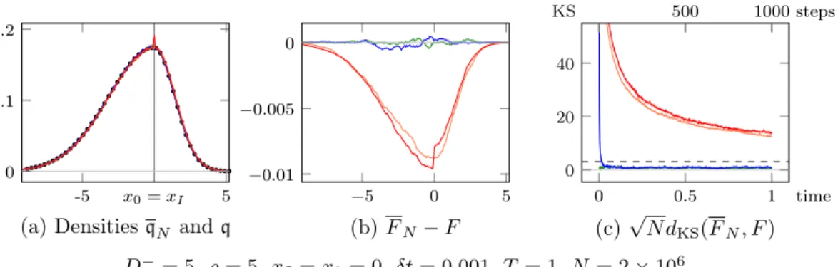
−5 0 5 −0.01 −0.005 0 (b) FN − F 0 0.5 1 0 20 40 500 1000 time steps KS (c) √N dKS(FN, F ) D−= 5, ρ = 5, x I = x0= 0, δt = 0.001, T = 1, N = 2× 10⁶
Figure 13: Plot of (a) the densities q𝑁 and q, (b) the difference between 𝐹𝑁 and 𝐹 , and (c) the normalized Kolmogorov-Smirnov distance 𝑀KS between the approximated and the true DF at time 𝑇 = 1.
5.1 Benchmark test Density: Numerical results
D− D+
xI = 0 injection
Figure 12: Medium for the Density test.
Density. Plot 𝑀KS defined by (12) as a function of 𝑡 and compare it with a threshold 𝑐𝛼 of the Kolmogorov-Smirnov statistics for a confidence level 𝛼, or to the value 𝑐𝛼 = 3 which corresponds to a level of risk 1− 𝛼 ≈ 3 × 10⁻⁷. First, we represent on Figure 13(a) the empirical densities of the four schemes after 1000 time steps of 2× 10⁶ of particles (𝛿𝑡 = 0.001). Qualitatively, SBM, Uffink and HMYLA seem to converge to the exact density (black dots). SBMlin presents a small peak at the discontinuity located at zero. However this sole qualitative comparison is not enough to quantify the bias of schemes. On Figure 13(b), we plot the differences between the approximated and the true DF. Now the bias of HMYLA and SBMlin is revealed. Figure 13(c) shows the evolution of the normalized Kolmogorov-Smirnov distance 𝑀KS :=
√
𝑁 𝑑KS(𝐹𝑁, 𝐹 ) with time. SBM is always close to the true density, Uffink converges rather quickly to the true one. On the other hand, for SBMlin and HMYLA — which share the same interpolation technique for computing the first hitting time of the interface — 𝑀KS is far above 3.
Now we represent on Figure 14 the evolution with time (and with number of steps) of the normalized Kolmogorov-Smirnov distance 𝑀KS:= √𝑁 𝑑KS(𝐹𝑁, 𝐹 ) for several choices of the input parameters.
0 0.05 0.1 0.15 0 5 10 15 20 5 10 15 time steps KS (a) ρ = 5, x0=−0.5, δt = 0.01, N = 105 0 0.05 0.1 0.15 0 20 40 5 10 15 time steps KS (b) ρ = 5, x0= 0, δt = 0.01, N = 105 0 0.05 0.1 0.15 0 10 20 5 10 15 time steps KS (c) ρ = 5, x0 = 0.5, δt = 0.01, N = 105 0 0.05 0.1 0.15 0 10 20 5 10 15 time steps KS (d) ρ = 20, x0 =−0.5, δt = 0.01, N = 105 0 0.05 0.1 0.15 0 20 40 0 5 10 15 time steps KS (e) ρ = 20, x0= 0, δt = 0.01, N = 105 0 0.05 0.1 0.15 0 5 10 15 0 5 10 15 time steps KS (f) ρ = 20, x0= 0.5, δt = 0.01, N = 105 0 0.05 0.1 0.15 0 5 10 15 5 10 15 time steps KS (g) ρ = 5, x0= 30, δt = 0.01, N = 105 0 0.05 0.1 0.15 0 50 100 5 10 15 time steps KS (h) ρ = 5, x0 = 0, δt = 0.01, N = 106 0 0.05 0.1 0.15 0 20 40 10 50 100 150 time steps KS (i) ρ = 5, x0 = 0, δt = 0.001, N = 105
Figure 14: Normalized Kolmogorov-Smirnov distance 𝑀KS for 𝐷− = 5, 𝜌 := 𝐷−/𝐷+ ∈ {5, 20} and a starting point 𝑥0 ∈ {−0.5, 0, 0.5}. The colors of the lines follows the convention of Table 5. When 𝛿𝑡 = 0.01, the interface layer is [−1.26, 0.56] for 𝜌 = 5, and [−1.26, 0.28] for 𝜌 = 20. We used 𝑁 = 105 particles. In the graph related to the Kolmogorov-Smirnov statistics, the dashed line has for abscissa 3, a choice justified in Section 3.1.2.
The method SBM is always close to the true density, whatever the parameters inputs. In the interface layer, Figures 14(b,e,h,i) confirm that Uffink converges to the true density after a few time steps and that SBMlin and HMYLA do not.
Increasing the number of steps (or equivalently decreasing 𝛿𝑡 as shown on Fig-ures 14(b,i)) decreases the bias of Uffink, HMYLA and SBMlin. The bias of Uffink will decrease to zero with the increase of number of steps (or decrease of 𝛿𝑡) while the bias of HMYLA and SBMlin will not decrease to zero.
In the zones of constant diffusivity (Figures 14(g)), SBM and SBMlin are superim-posed exactly as they move the particles with the same Gaussian dynamics. They replicate the exact dynamics of the particle, up to events of exponentially small probability (see the discussion on the interface layer above). Similarly, Uffink and HMYLA are superimposed as they both move the particles with a uniform step. They replicate the exact dynamics after a few time steps.
The change of zones is illustrated on Figures 14(a,c,d,f). The bias of SBMlin and HMYLA is revealed while more particles enter the interface layer (increase of 𝑀KS). Increasing the number of particles increases the bias of the schemes as illustrated on Figure 14(h).
This density benchmark test is important as it reveals the bias of schemes. However it does not provide any information on the effects of the bias on the computations of micro- and macroscopic quantities of interest. Moreover it does not allow to distinguish between SBMlin and HMYLA schemes.
5.2 Benchmark test Layer: Numerical results
D0 Dm D0
periodic periodic
0 L
0 L/2− ` L/2 + `
Figure 15: Medium for the Layer test.
Layer. For a time 𝑡 large enough, plot 𝐾𝑁(𝑡, 𝑦) defined by (14) and compare it with 𝑦 ∈ [0, 1] ↦→ ±𝑑𝛼√︀𝑦(1 − 𝑦) for a confidence level 𝛼 with 𝑑𝛼 defined by (10).
0 0.2 0.4 0.6 0.8 1 −4 −2 0 2 4 0 0.2 0.4 0.6 0.8 1 −4 −2 0 2 4 0 0.2 0.4 0.6 0.8 1 −4 −2 0 2 4 0 0.2 0.4 0.6 0.8 1 −4 −2 0 2 4 0 0.2 0.4 0.6 0.8 1 −4 −2 0 2 4 0 0.2 0.4 0.6 0.8 1 −4 −2 0 2 4 0 0.2 0.4 0.6 0.8 1 −4 −2 0 2 4 0 0.2 0.4 0.6 0.8 1 −4 −2 0 2 4 0 0.2 0.4 0.6 0.8 1 −4 −2 0 2 4 0 0.2 0.4 0.6 0.8 1 −4 −2 0 2 4 0 0.2 0.4 0.6 0.8 1 −4 −2 0 2 4 0 0.2 0.4 0.6 0.8 1 −4 −2 0 2 4 (a) ρ = 2.5 (b) ρ = 5 (c) ρ = 7.5 (d) ρ = 10 (e) ρ = 12.5 (f) ρ = 15 (g) ρ = 17.5 (h) ρ = 20 (i) ρ = 100 (j) ρ = 250 (k) ρ = 500 (l) ρ = 750
Figure 16: Layer — Plot of 𝑥 ↦→ 𝐾𝑁(𝑡, 𝑥) for the four methods: SBM,
Uffink, HMYLA and SBMlin and comparison with the 99 %-confidence band
𝑦↦→ ±𝑑0.99√︀𝑦(1 − 𝑦) at 𝑇 = 10.
SMBlin method fails in preserving the uniform distribution of the particles with time. On the contrary, SBM, Uffink and HMYLA methods pass this test.
5.3 Benchmark test Bimaterial: Numerical results
D− D+
reflecting reflecting
0 L/2 injection L