HAL Id: hal-00714702
https://hal.archives-ouvertes.fr/hal-00714702
Submitted on 5 Jul 2012
HAL is a multi-disciplinary open access
archive for the deposit and dissemination of
sci-entific research documents, whether they are
pub-lished or not. The documents may come from
teaching and research institutions in France or
abroad, or from public or private research centers.
L’archive ouverte pluridisciplinaire HAL, est
destinée au dépôt et à la diffusion de documents
scientifiques de niveau recherche, publiés ou non,
émanant des établissements d’enseignement et de
recherche français ou étrangers, des laboratoires
publics ou privés.
Condon domain phase diagram for silver
Roman Kramer, V. S. Egorov, V. A. Gasparov, A. G. M. Jansen, W. Joss
To cite this version:
Roman Kramer, V. S. Egorov, V. A. Gasparov, A. G. M. Jansen, W. Joss. Condon domain phase
diagram for silver. Low Temperature Physics, American Institute of Physics, 2011, 37 (1), pp.39-44.
�10.1063/1.3549167�. �hal-00714702�
R. B. G. Kramer,1, 2, 3 V. S. Egorov,1, 2, 4 V. A. Gasparov,5 A. G. M. Jansen,6 and W. Joss1, 2, 7
1LNCMI, CNRS, BP 166, 38042 Grenoble Cedex 9, France
2Max-Planck-Institut f¨ur Festk¨orperforschung, Heisenbergstraße 1, 70569 Stuttgart, Germany 3Institut N´eel, CNRS, Universit´e Joseph Fourier, BP 166, 38042 Grenoble Cedex 9, France
4Russian Research Center ”Kurchatov Institute”, 123182 Moscow, Russia
5Institute of Solid State Physics, Russian Academy of Sciences, 142432 Chernogolovka, Russia
6Service de Physique Statistique, Magn´etisme, et Supraconductivit´e, INAC, CEA, 38054 Grenoble Cedex 9, France 7Universit´e Joseph Fourier, BP 53, 38041 Grenoble Cedex 9, France
(Dated: February 22, 2010)
We present the Condon domain phase diagram for a silver single crystal measured in magnetic fields up to 28 T and temperatures down to 1.3 K. A standard ac method with a pickup coil system is used at low frequency for the measurements of the de Haas-van Alphen effect (dHvA). The transition point from the state of homogeneous magnetization to the inhomogeneous Condon domain state (CDS) is found as the point where a small irreversibility in the dHvA magnetization arises, as manifested by an extremely nonlinear response in the pickup voltage showing threshold character. The third harmonic content in the ac response is used to determine with high precision the CDS phase boundary. The experimentally determined Condon domain phase diagram is in good agreement with the theoretical prediction calculated by the standard Lifshitz-Kosevich (LK) formula.
PACS numbers: 75.45.+j, 71.70.Di, 75.60.-d
I. INTRODUCTION
The formation of dia- and paramagnetic domains has been predicted by Condon1 to occur in non-magnetic pure metals by considering the collective interaction be-tween the electrons on Landau-quantized energy levels in the de Haas-van Alphen (dHvA) effect. These domains corresponding to an inhomogeneous magnetization are commonly called Condon domains. The domain forma-tion results from a self-consistent treatment of the oscil-lating dHvA magnetization M due to the orbital quan-tization of the electronic system in the total magnetic induction B = µ0(H + M ), where M = M (B) depends on the total induction B in an applied magnetic field H. Following the Pippard-Shoenberg concept of mag-netic interaction2,3where the electrons experience the in-fluence of the magnetic field induced magnetization of all neighboring electrons, a thermodynamic instability arises when the dHvA amplitude becomes large enough, i.e., the differential susceptibility
χ = µ0∂M
∂B > 1. (1) This condition corresponds to the situation where the amplitude of the magnetization amplitude becomes com-parable to the magnetic field period of the dHvA effect. For sufficiently strong magnetization amplitudes, this in-stability condition, rewritten like µ0∂H/∂B = 1 − χ < 0, occurs in a certain field interval within the paramag-netic part of each dHvA cycle. In these field intervals, where µ0∂H/∂B < 0, the induction as function of the ap-plied field B(H) is multi-valued, like the van der Waals isotherm for a real gas. The system avoids this instability in the same way as the real gas. For an infinite long
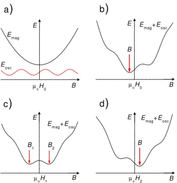
rod-like sample (demagnetization factor n = 0), the induc-tion B undergoes a discontinuous transiinduc-tion between the two stable states with the induction B1and B2 at a cer-tain applied field H, like the liquid-gas specific volumes change discontinuously at the equilibrium vapor pressure. Both stable states B1 and B2 correspond to the same free energy and the inductions in the instability interval (B1, B2) are never realized. Figure 1(a) shows schemat-ically the magnetization energy Emag= 1
2µ0(B − µ0H)
2 for n = 0 and the oscillating dHvA energy described by the LK-formula Eosc= a cos(2πF/B) to its simplest ap-proximation with a the oscillation amplitude and F the dHvA frequency. The sum of both energies as function of B is shown for three different magnetic fields in Fig.1(b)-(d). Usually, there is only one minimum in the total energy for a given applied magnetic field and the system will assume this value of B. However if the curvature of the Emag is smaller than the curvature of Eosc two minima coexist at an applied field H1[Fig.1(c)] and the induction will jump discontinuously from the value B1to B2 when sweeping the magnetic field through H1.
For a plate-like sample, oriented normal to the ap-plied magnetic field H (n = 1), the boundary condi-tion B = µ0[H + (1 − n)M] = µ0H is required even in the interval B1 < µ0H < B2. Therefore, the induction B can not change discontinuously and a homogeneous state is no longer possible. The plate breaks up into do-mains of opposite magnetization. The volume fractions of the domains with the respective inductions B1 and B2 are adjusted in a way that for the average induction of the sample B = µ0H is fulfilled1. The regions with B1 < µ0H are diamagnetic, those with B2 > µ0H are paramagnetic. The domain walls between the phases B1 and B2 run parallel to H across the plate. In contrast to
2
d
)
c
)
E B µ0H0 Emag+Eosc Bb
)
a
)
E B B2 B1 Emag+Eosc µ0H1 E B µ0H2 Emag+Eosc B E B Emag Eosc µ0H0FIG. 1: (Color online) (a) Schematic representation of the magnetization energy Emag and the dHvA-energy Eosc as
function of B for n = 0. (b)-(d) Sum of these energies for three applied magnetic fields H0< H1< H2. If the curvature
of the parabola is smaller than the curvature of the oscillating energy two minima coexist at H1. This leads to
discontinu-ous jump of the induction when sweeping the magnetic field through H1.
magnetic domains in common ferro- and antiferromag-netism, Condon domains do not have their origin in the interaction of electrons via their spin moments, but via their orbital motion.
For a sample shape with intermediate demagnetization factor, 0 < n < 1, the above mentioned interval of mag-netic field B1< µ0H < B2with the occurrence of the in-stability will be reduced compared to the plate-like sam-ple with the field range of this interval proportional to n. Therefore, samples of arbitrary shape will still show the nonuniform domain state with the same dia- and para-magnetic phases, B1 and B2, whose domain structure might however be more complex.
Besides the analogy with the van der Waals gas, there is a close analogy of the CDS with the intermediate state of type-I superconductors, where the same bound-ary condition of a magnetic field applied to a sample of nonzero demagnetization factor leads to the formation of alternating domains in the normal and superconducting state. Condon domains, however, have the unique feature that the transition between the uniform and the inhomo-geneous domain state occurs periodically in subsequent dHvA oscillations.
Equation 1 defines the boundary between the uniform and the Condon domain state. The resulting CDS phase diagram in the (H, T ) plane can be predicted by means
of the Lifshitz-Kosevich (LK) formula for the oscillatory magnetization of the dHvA signal using the Fermi sur-face parameters, like the curvature A′′= ∂2A/∂k2of the Fermi surface cross section A and the effective mass m∗, and the Dingle temperature TD as a parameter for the impurity-scattering damping of the signal4.
Up to now, Condon domains have been observed by different experimental methods: by NMR5, muon spin rotation (µSR) spectroscopy6,7 and, more recently, by local Hall probes8. All experimental observations have in common that two distinct inductions B1 and B2 or an induction splitting δB = B2− B1 are measured at a given applied field H and temperature T . However, these measurements yielded only a few points well inside the (H, T ) diagram where Condon domains exist that could be compared with the theoretically predicted diagram. As a consequence, for example, the data on beryllium ob-tained by µSR required new phase diagram calculations with a modified LK-formula for the susceptibility9. The exact determination of the CDS phase boundary, where δB approaches zero, is difficult and time-consuming with a difference measurement of B1 and B210.
It was shown recently that a small hysteresis occurs in the measured dHvA signal upon passing the CDS phase boundary11. Due to the irreversible magnetization, an extremely nonlinear response to a small modulation field arises in standard ac susceptibility measurements. The out-of-phase signal and the third harmonic of the pickup voltage rise steeply at the transition point to the CDS. The threshold character of these quantities offers there-fore a possibility to measure a Condon domain phase di-agram. One should note that the third harmonic of the susceptibility is commonly used as a very sensitive tool to detect phase boundaries also of other systems like e.g. the vortex-glass transition in superconductors12.
In this article we determine the Condon domain phase diagram for silver using the third harmonic of the ac sus-ceptibility for the detection of the nonlinear magnetic response. It was shown earlier13 that detailed calcula-tions of the magnetoquantum oscillacalcula-tions in silver based on the LK-formula are in good agreement with experi-mental dHvA data up to 10 T. This is certainly due to the nearly spherical Fermi surface of silver. Expecting a good agreement with the theoretically determined CDS phase diagram, we applied to silver this first detailed de-termination of the phase diagram.
II. EXPERIMENTAL
The measurements were performed on a high quality silver single crystal of 4.1 × 2.1 × 1.0 mm3. The sample was cut from the same piece than the sample used for the direct observation of Condon domains using local Hall probe detection8. The sample preparation is described in detail elsewhere14,15. The sample has a residual resis-tance ratio R300 K/R4.2 K = 1.6×10⁴, measured by the contactless Zernov-Sharvin method16. The high quality
of the sample results in a very low Dingle temperature, which was estimated from standard dHvA analysis to be about TD= 0.2 K yielding an electronic mean free path of about 0.8 mm.
A standard ac modulation method with a compensated pickup coil system was used. Both pickup coils are identi-cal and consist of about 400 turns. A long coil wound by a copper wire produced the modulation field with vari-able amplitude at frequencies of 20 − 200 Hz. The pickup voltage was simultaneously measured by two lock-in am-plifiers on the first and on higher harmonics. The mea-surements were performed in a superconducting coil up to 16 T as well as in a resistive coil up to 28 T at tem-peratures of 1.3 − 4.2 K. The long side of the sample was parallel to the [100]-axis of the single crystal and was slightly tilted (∼ 5 deg) with respect to the direction of the applied magnetic field so that only the dHvA fre-quency from the ”belly” orbit of 47300 T existed in the frequency spectrum.
The method of nonlinear detection, we use here, is ap-plied to determine for the first time a CDS phase dia-gram over a broad range of temperatures and magnetic fields. Therefore, we will present carefully the technical details of the measurements in order to show the robust-ness of the phase diagram determination with respect to changing experimental parameters and measurement conditions.
III. EVIDENCE OF HYSTERESIS IN SILVER
The employed method to determine a Condon domain phase diagram is based on the appearance of hysteresis in the CDS which was first discovered on beryllium11. Hys-teresis appears at the phase transition to the CDS and this results in some radical changes in the response to an ac modulation field. In the following, we will show that the characteristic nonlinear features in the ac response, as found in beryllium, are also observed in silver.
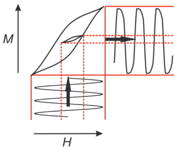
In presence of hysteresis the amplitude of the suscep-tibility, normalized on the modulation level, depends on the modulation amplitude. This is expected to occur when the modulation level is of the order of the hysteresis loop width. The schematic representation of a hysteresis loop in Fig. 2 explains this nonlinear response to an ac field modulation. As a result, after the transition to the CDS, the positive (paramagnetic) part of the susceptibil-ity turns out to be reduced. From a comparison of two normalized susceptibilities, one measured with high and the other with low modulation level, we can in principle find where the amplitude reduction starts and thereby the transition point to the CDS.
Figure 2 shows as well that the response to a sinusoidal field modulation becomes window shaped and is slightly shifted in phase with respect to the input. Therefore, both the third harmonic and the out-of-phase signal of the pickup voltage increase steeply when the CDS phase boundary is crossed11. This threshold behavior offers
M
H
FIG. 2: (Color online) Schematic representation of two minor hysteresis loops. The ac response upon field modulation is window-like and slightly shifted in phase. The normalized response (apparent susceptibility) decreases sharply when the modulation amplitude becomes of the order of the hysteresis loop width.
a simple way to determine the transition point of the CDS. The major advantage of third harmonic and out-of-phase part measurements is that only one magnetic field or temperature sweep through the transition is needed.
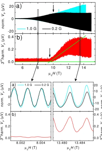
Figures 3 and 4 show the above discussed nonlinear features in the pickup signal at constant temperature T = 2.7 K measured in the superconducting coil. Fig-ure 3(a) shows two traces of the normalized pickup volt-age, i.e. the susceptibility, obtained in the same con-ditions with 1.0 G and 0.2 G modulation amplitude at 160 Hz modulation frequency. In principle, both mod-ulation levels are small enough compared to the dHvA period of about 20 G at 10 T that identical traces are ex-pected for the susceptibility. The expanded view around 8 T, which is outside the CDS, shows that the normal-ized signals are indeed identical. For higher fields, on the other hand, the upper part of the susceptibility wave-form, measured with the smaller modulation level, is re-duced. The expanded view around 13.5 T shows that the signals are identical except for the positive part of the oscillation. This implies that at this part of the dHvA oscillation the magnetization is irreversible and there is a small hysteresis loop. The width of the hysteresis loop is of the order of 0.2 G.
A similar decrease of the normalized response was ob-served earlier17 on silver at low temperatures. Unfortu-nately, because of the absence of the experimental pa-rameters, this study can be compared only qualitatively with our data.
The magnetic field where the normalized pickup volt-ages start to differ between low and high modulation level is marked approximately by an arrow in Fig. 3(a). We obtain for the critical magnetic field µ0Hc1= 10.0 T.
Figure 3(b) shows the behavior of the third harmonic which was simultaneously measured with the first har-monic response in Fig. 3(a) for 0.2 G modulation
am-4 6 8 10 12 14 0.0 0.2 0.4
b)
3 r d h a r m . VP ( µ V ) µ0H (T) -20 0 20 1.0 G 0.2 Ga)
n o rm . VP ( µ V ) 13.480 13.484 0.0 0.2 0.4 8.002 8.004 0.0 0.2 0.4 3 r d h a rm . VP ( µ V ) µ0H (T) -20 -10 0 10 20 n o rm . V P ( µ V ) -2 0 2 1.0 G 0.2 G a) n o rm . VP ( µ V ) b) 3 r d h a rm . VP ( µ V ) µ0H (T)FIG. 3: (Color online) (a) Pickup voltage normalized on the modulation level for low and high modulation level. Up to about 10 T the response is linear with respect to the modula-tion level. (b) Third harmonic of the pickup voltage measured at 0.2 G modulation amplitude showing that starting from 9.5 T the harmonic content in the response increases steeply. Lower part of the figure shows respective zooms. Both data measured at 2.7 K.
plitude. For magnetic fields lower than the critical field there is only noise. At the transition to the CDS hystere-sis arises and the third harmonic increases very steeply. This is nicely seen in the respective expanded views. The critical field of the CDS phase boundary can be obtained as the intersection of the two straight lines shown in Fig. 3(b). Here, the critical field is found as µ0Hc2= 9.6 T.
The amplitude of the third harmonic is expected to go to zero in each diamagnetic part of the dHvA period be-cause the sample magnetization is here homogeneous and without hysteresis. The presented behavior in Fig. 3(b) does not go to zero exactly which is certainly the result of a small rectification effect or, what is the same, the result of phase smearing of the oscillation signal. The homogeneity of the coil is about 30 ppm in a sphere with 1 cm diameter which may result in a field inhomogeneity
8 10 12 14 -0.4 0.0
b)
Im V P ( µ V ) µ 0H (T) -180 0 180a)
a n g le 3 rd h a rm . Vp ( d e g )FIG. 4: (Color online) (a) Phase angle of the third harmonic showing clearly the transition between noise outside the CDS and a fixed phase in the CDS. (b) The out-of-phase part of the first harmonic response changes due to the arising hysteresis. Both data measured at 2.7 K and 0.2 G modulation level.
of about 1 G in the sample volume at 10 T. Therefore, the transition to the CDS does not occur simultaneously in the whole sample. This effect will be much bigger in a resistive coil where the homogeneity is 20 times worse. However, we will see below, that the third harmonic rec-tification does not affect the determination of the critical field of the CDS.
In Fig. 4(a) the phase angle of the third harmonic is shown for the same conditions like in Fig. 3. For mag-netic fields where the amplitude of the third harmonic is below the noise level its phase angle is not determined. Therefore, the phase varies between −180 to +180 de-gree. With the appearance of a third harmonic signal at the transition to the CDS the phase becomes finite. This passage has a threshold character as well. The arrow in Fig. 4(a) shows the position of the threshold which yields the critical field µ0Hc3= 9.7 T.
The behavior of the out-of-phase part of the first har-monic response, shown in Fig. 4(b), offers another pos-sibility to determine the critical field. In the uniform state, without domains, the imaginary part is small and varies smoothly especially at low magnetic field due to the magnetoresistance and changing eddy currents. After the transition to the CDS the out-of-phase signal changes rapidly. The transition point can be found as the inter-section of two lines, as it is shown in Fig. 4(b). Here, we obtain for the critical field µ0Hc4= 9.4 T.
A comparison of the values Hc1...c4 for the transition field at 2.7 K shows that they are very close. We note that
the critical field of about 10 T agrees roughly with the phase boundary found in the Hall probe experiments8. All above presented methods could, in principle, be used to determine the phase boundary of the CDS. The first method (fig. 3(a)) requires at least two field sweeps. Mea-surements of the out-of-phase part (fig. 4(b)) are not precise, due to the high conductivity of silver and the resulting eddy currents (The situation might be different in a less conducting metal). Therefore, for silver the third harmonic measurements to determine the CDS phase dia-gram are preferred. Moreover, we will see below that the obtained values with the third harmonic for the phase boundary (H, T ) do not depend drastically on the fre-quency and amplitude of the field modulation which of-fers the possibility to measure in noisier conditions. The found scattering in the values of the transition fields ob-tained from the different methods gives an uncertainty of about ±0.5 T in the transition fields.
IV. PHASE DIAGRAM
Because of the increased noise level in the water-cooled resistive magnets, we needed to increase the signal-to-noise ratio by using rather high modulation frequencies ≈160 Hz and higher modulation amplitudes, 1.0 G and more. In the following we check whether the modulation frequency and amplitude can be varied without chang-ing the value of the critical field deduced from the third harmonic response.
Modulation amplitudes of the order of the width of the hysteresis loop are required to resolve the amplitude re-duction in the normalized pickup voltage in Fig. 3(a). For the third harmonic signal, as shown in Fig. 2, the non-linear features persist up to high modulation amplitudes. Figure 5 shows traces with 0.2 and 1.0 G modulation am-plitude. For 1.0 G modulation amplitude there is a very small third harmonic signal before the transition to the CDS takes place. This small contribution to the third harmonic is due to the nonlinearity of the dHvA effect itself3. Nevertheless, the position of the sharp increase remains unchanged.
Figure 6 shows that increasing the modulation ampli-tude up to 10 G and varying the modulation frequency by a factor four between 40 Hz and 160 Hz does not change the position of the critical field, either. The results pre-sented here were obtained in the resistive magnet. The measurements were made at low temperatures in order to compare them with data obtained in the superconducting magnet.
All results for the CDS transition points obtained in the superconducting and the resistive magnets are pre-sented in Fig. 7. The critical fields for each temperature are found as the field where the third harmonic response starts to arise like in Fig. 6. One should note that near the flat maximum of the phase diagram T -sweep mea-surements would be in principle better. The solid line in Fig. 7 is the CDS boundary calculated for silver using the
6 8 10 12 14 0.0 0.2 0.4 0.2 G
b)
3 r d h a rm . V P ( µ V ) µ0H (T) 0 1 2a)
1.0 GFIG. 5: (Color online) Third harmonic response for two mod-ulation levels measured in a superconducting coil at a modu-lation frequency of 160 Hz at 2.7 K. The same critical field is found from the steep increase.
4 6 8 10 0 2 4 2 4 6 0 1 10.0 G 5.0 G 2.5 G 3 r d h a rm . V P ( µ V ) µ0H (T) T = 2.0 K
a)
b)
161 Hz 81 Hz 40 Hz 3 r d h a rm . V P ( µ V ) µ0H (T) T = 1.4 KFIG. 6: Third harmonic response measured after averaging over the oscillations in a resistive coil for different modulation amplitudes (a) and modulation frequencies (b).The critical field values obtained at a given temperature are independent on modulation frequency and amplitude.
LK-formula for the susceptibility criterion χ = 1 with a Dingle temperature of TD = 0.2 K for our sample13,18. For comparison, theoretical diagrams for TD= 0.1 K and 0.8 K are shown in Fig. 7.
A good agreement of the phase diagram predictions based on the LK-formula with our data can be seen for a Dingle temperature TD= 0.2 K. Data points obtained in superconducting and resistive magnets overlap which supports that the different measurement conditions did not affect the precise determination of the phase bound-ary.
6 0 10 20 30 40 50 0 1 2 3 4 5 TD = 0.1 K TD = 0.8 K resistive m agnet superconducting m agnet TD = 0.2 K T (K ) µ0H (T)
FIG. 7: (Color online) Phase diagram in the (H, T ) plane for silver. Experimental points from the superconducting and resistive magnet. The solid line is the CDS boundary calcu-lated by the LK-formula for TD= 0.2 K13,18. The dashed and
the dotted lines correspond to TD = 0.8 K and TD = 0.1 K,
respectively.
V. CONCLUSION
Like previously observed in beryllium11, we have shown that hysteresis appears in silver in the Condon
domain state. This substantiates that hysteresis is likely to occur in all pure metals that exhibit Condon domains. The hysteresis leads to with threshold character arising extremely nonlinear response to a modulation field. In particular, the third harmonic response to a modulation field increases sharply upon entering into the Condon do-main state. This offered the possibility to determine eas-ily the CDS phase boundary with high accuracy.
The critical fields obtained from the third harmonic of the pickup signal of the ac modulation technique, turned out to be independent on changes of the modulation fre-quency and amplitude. Due to this independence this method could be used with higher modulation frequen-cies in pulse magnetic fields.
Very good agreement of the CDS phase diagram is found with calculations of the dHvA signal based on the LK-theory. This agreement shows that the LK-formula describes well the field dependent magnetization of the nearly spherical Fermi surface of silver. Furthermore, the agreement demonstrates that the described method is correct for the determination of the CDS phase dia-gram.
Acknowledgments
We are grateful to I. Sheikin and V. P. Mineev for fruitful discussions.
1 J. H. Condon, Phys. Rev. 145, 526 (1966). 2 A. B. Pippard, Proc. R. Soc. A: 272, 192 (1963).
3 D. Shoenberg, Magnetic oscillations in metals (Cambridge
University Press, Cambridge, 1984).
4 A. Gordon, I. D. Vagner, and P. Wyder, Adv. Phys. 52,
385 (2003).
5 J. H. Condon and R. E. Walstedt, Phys. Rev. Lett. 21,
612 (1968).
6 G. Solt, C. Baines, V. S. Egorov, D. Herlach,
E. Krasnoperov, and U. Zimmermann, Phys. Rev. Lett. 76, 2575 (1996).
7 G. Solt and V. S. Egorov, Physica B 318, 231 (2002). 8 R. B. G. Kramer, V. S. Egorov, V. A. Gasparov, A. G. M.
Jansen, and W. Joss, Phys. Rev. Lett. 95, 267209 (2005).
9 G. Solt, Solid State Commun. 118, 231 (2001).
10 G. Solt, C. Baines, V. S. Egorov, D. Herlach, and U.
Zim-mermann, Phys. Rev. B 59, 6834 (1999).
11 R. B. G. Kramer, V. S. Egorov, A. G. M. Jansen, and
W. Joss, Phys. Rev. Lett. 95, 187204 (2005).
12 T. Klein, A. Conde-Gallardo, J. Marcus, C.
Escribe-Filippini, P. Samuely, P. Szabo, and A. G. M. Jansen, Phys. Rev. B 58, 12411 (1998).
13 R. B. G. Kramer, V. S. Egorov, A. Gordon, N. Logoboy,
W. Joss, and V. A. Gasparov, Physica B 362, 50 (2005).
14 V. A. Gasparov, Sov. Phys. JETP 41, 1129 (1975), [Zh.
Eksp. Teor. Fiz. 68, 2259 (1975)].
15 V. A. Gasparov and R. Huguenin, Adv. Phys. 42, 393
(1993).
16 V. B. Zernov and Y. V. Sharvin, Sov. Phys. JETP 9, 737
(1959), [Zh. Eksp. Teor. Fiz. 36, 1038 (1959)].
17 J. L. Smith and J. C. Lashley, J. Low Temp. Phys. 135,
161 (2004).
18 A. Gordon, M. A. Itskovsky, and P. Wyder, Phys. Rev. B