HAL Id: hal-01344084
https://hal.archives-ouvertes.fr/hal-01344084
Submitted on 11 Jul 2016
HAL is a multi-disciplinary open access
archive for the deposit and dissemination of
sci-entific research documents, whether they are
pub-lished or not. The documents may come from
teaching and research institutions in France or
abroad, or from public or private research centers.
L’archive ouverte pluridisciplinaire HAL, est
destinée au dépôt et à la diffusion de documents
scientifiques de niveau recherche, publiés ou non,
émanant des établissements d’enseignement et de
recherche français ou étrangers, des laboratoires
publics ou privés.
Efficient Operations On MDDs For Building Constraint
Programming Models
Guillaume Perez, Jean-Charles Régin
To cite this version:
Guillaume Perez, Jean-Charles Régin. Efficient Operations On MDDs For Building Constraint
Pro-gramming Models. IJCAI 2015, Jul 2015, Buenos Aires, Argentina. �hal-01344084�
Efficient Operations On MDDs For Building Constraint Programming Models
Guillaume Perez and Jean-Charles Régin
Université Nice-Sophia Antipolis, I3S UMR 7271, CNRS, France
[email protected]; [email protected]
Abstract
We propose improved algorithms for defining the most common operations on Multi-Valued Deci-sion Diagrams (MDDs): creation, reduction, com-plement, intersection, union, difference, symmetric difference, complement of union and complement of intersection. Then, we show that with these algo-rithms and thanks to the recent development of an efficient algorithm establishing arc consistency for MDD based constraints (MDD4R), we can simply solve some problems by modeling them as a set of operations between MDDs. We apply our approach to the regular constraint and obtain competitive re-sults with dedicated algorithms. We also experi-ment our technique on a large scale problem: the phrase generation problem and we show that our approach gives equivalent results to those of a spe-cific algorithm computing a complex automaton.
1
Introduction
MDDs become more and more used in constraint program-ming. The recent development of MDD4R, an efficient and fully incremental arc consistency algorithm [Perez and Régin, 2014], seems to show that MDD constraints are competitive with Table constraints. We can see a table constraint as a set of disjoint paths (each path corresponding to a tuple) that are preceded by an initial node and whose last node is linked to a terminal node, that is as a particular MDD which is not com-pressed. The compression process may dramatically reduce the size of the underlying graph and so the complexity of the arc consistency algorithm maintaining it.
In this paper, we aim at showing that we can expect to di-rectly use MDDs with the help of MDD4R for establishing arc consistency of some complex constraints like the regu-lar constraint or constraints based on dynamic programming like the knapsack constraint. We propose to explicitly create and work with MDDs instead of dedicated algorithms associ-ated with the constraints. The advantage of dealing directly with MDDs is that they are always reduced after their creation so MDD4R may outperform dedicated algorithms, which do not perform this operation. Currently, the complexity of the existing algorithms prevents us from using them for solving
some problems. For instance, phrase generation problem in-volves domains having more than d = 10, 000 values. Thus, we cannot use an algorithm whose time or space complexity is mainly based on Ω(nd), where n is the number of nodes of the MDDs. Therefore, we need to improve the algorithms performing the main operations on MDDs: creation, reduc-tion and combinareduc-tions.
The new creation algorithm we propose, exploits the origin of the definition of the MDD. If the MDD represents an au-tomaton (like with a regular constraint) or a repeated pattern (like with dynamic programming), then its creation may be sped-up.
Then, we introducePREDUCEa new algorithm for reduc-ing an MDD, i.e. eliminatreduc-ing nodes that are not lyreduc-ing on a path from the initial node to the terminal node. Our algorithm proceeds by layers and uses a simple an original procedure for gathering equivalent nodes in order to keep the time complex-ity in the size of the neighborhood of nodes instead of being bounded by Ω(d). This new algorithm improves the Cheng and Yap’s one [Cheng and Yap, 2010]. It is also conceptually simpler.
At last, we present a generic algorithm for computing basic combinations of MDDs. Our algorithm is based on graph op-erations that are made on the underlined graph of the MDDs. Each combination, such as intersection, union, difference, symmetric difference, is defined by applying a specific op-eration for each node of the MDDs depending on the fact that two nodes have an arc labeled by a value or not. In that way, we obtain a really short and powerful algorithm. Then by defining some operations for each node of each layer we in-stantiate our generic algorithm and compute the desired com-bination.
Before concluding, we present some experiments showing some strong improvements brought by our algorithms. In par-ticular, we show that we can gain orders of magnitude for the reduction of MDDs and that we are able to compute a dozen of intersections of MDDs having millions of nodes, hundreds millions of arcs and ten thousand values. Then, the appli-cation of MDD4R on MDDs leads to computational times equivalent to those of dedicated algorithms.
2
Background
Multi-valued decision diagram (MDD) is a method for rep-resenting discrete functions. It is a multiple-valued
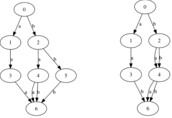
exten-Mdd before reduction Mdd after reduction
Figure 1: Reduction of an MDD. Nodes without successors are deleted (e.g. node 4). Equivalent nodes are merged (e.g. nodes 3 and w2).
sion of BDDs [Bryant, 1986]. An MDD, as used in CP [An-dersen et al., 2007; Hadzic et al., 2008; Hoda et al., 2010; Bergman et al., 2011; Gange et al., 2011], is a rooted di-rected acyclic graph (DAG) used to represent some multi-valued function f : {0...d − 1}r → {true, f alse}, based on a given integer d (See Figure 1.). Given the r input vari-ables, the DAG representation is designed to contain r layers of nodes, such that each variable is represented at a specific layer of the graph. Each node on a given layer has at most d outgoing arcs to nodes in the next layer of the graph. Each arc is labeled by its corresponding integer. The final layer is represented by the true terminal node (the false terminal node is typically omitted). There is an equivalence between f (v1, ..., vr) = true and the existence of a path from the
root node to the true terminal node whose arcs are labeled v1, ..., vr. Nodes without any outgoing arc or without any
incoming arc are removed.
In an MDD constraint, the MDD models the set of tuples satisfying the constraint, such that every path from the root to the true terminal node corresponds to an allowed tuple. Each variable of the MDD corresponds to a variable of the con-straint. An arc associated with an MDD variable corresponds to a value of the corresponding variable of the constraint.
We will denote by L[i] the nodes in layer i and by ω+(x) the set of outgoing arcs of the node x.
3
Creation
Some constraints like table, regular or knapsack may be ex-plicitly represented by an MDD. The advantage of this ap-proach is that the MDD is reduced after its creation and arc consistency algorithms may benefit from its reduction. The drawbacks are the time for creating the MDD and the com-plexity of the filtering algorithm. We will present later some experiments showing that MDD4R is competitive with dedi-cated algorithms. Now, we propose to show how the creation may be accelerated.
Cheng and Yap [Cheng and Yap, 2010] have proposed an algorithm for creating an MDD from a table contraint. In this case, a trie data structure is created and it is reduced in order to obtain an MDD. We introduce two new ways for creating
an MDD: from an automaton and from a pattern.
Creation from an automaton. The regular constraint [Pe-sant, 2004] deals with an automaton from which it deduces the allowed tuples. It corresponds to a set of ternary transi-tion constraints [Beldiceanu et al., 2004]: T (δ, Qi, xi, Qi+1),
where δ is a common transition function, Qiand Qi+1 two
state variables and xia variable. A transition constraint
de-fines for which values of xiwe can go from a state q to a state
q0. Note that δ is a function, so there is only one value of q0 for a couple (v, q) with v ∈ xi and q ∈ Qi. First, we create
the nodes. Each layer i is associated with the variable Qiand
has as many nodes as there are possible states. Each node of the layer i corresponds to a pair (Qi, q) where q is a possible
state. Thus, for each tuple (q1, v, q2) satisfying the
transi-tion constraint we create for each layer i, an arc from node (Qi, q1) to node (Qi+1, q2) labeled by v. If i = r then all
nodes (Qi+1, q2) represent the true terminal node. Note that
we do not need to know all tuples before creating the MDD. It is important to remark that each layer of the MDD cannot have more arcs than the number of tuples in the transition constraint. So, using explicitly an MDD does not introduce any additional cost if the arc consistency algorithms of the ternary constraints do not share a global transition table.
Creation from a pattern. In some cases, the transition constraint depends on the variables it involves and Function δ is not globally shared. Precisely we have a δifunction for
each layer i. The layers are built successively by applying the transition constraint. Each node of the MDD is associ-ated with an information that depends on the layer. For in-stance for the knapsack constraint [Trick, 2003], the informa-tion corresponds to the current value of the sum from the root to the current node (every path to the node leads to the same value). This information can be a scalar but also be more complex. Note that we may have an exponential number of nodes. However, only one layer in memory is sufficient for building the MDD.
4
Reduction
The reduction of an MDD is one of the most important op-erations. It consists of merging equivalent nodes, i.e. nodes having the same set of outgoing neighbors associated with the same labels. Figure 1 gives an example of reduction.
A reduction algorithm for BDDs has been given by Bryant [Bryant, 1986]. It proceeds by layer from the bottom to the top, considers each node x successively and tries to find an-other node x0 that can be merged with it. It has a time com-plexity in O(n log(n)) for a BDD having n nodes. We could adapt it for MDDs by associating with each node its list of neighbors. Note that the neighbor of a node can be seen as a couple (node, label). Then, by ordering the neighbors lists, we can maintain an ordered list of nodes. At the beginning the list of nodes contains all nodes and then we reduce it by merging nodes having the same list of neighbors. If we have n nodes then the complexity of this algorithm will be in O(n log(n)d) because the comparison is in O(d) for an MDD.
Cheng and Yap [Cheng and Yap, 2010] have proposed an-other algorithm (mddify) that also considers the nodes
suc-cessively and searches for merging nodes. However, it pro-ceeds differently than Bryant’s algorithm in order to improve the complexity. It uses a dictionary for speeding up the search for a similar node of a given node. Chang and Yap do not detail their algorithm and claim that the search for a similar node can be computed in O(d). There are two ways for im-plementing such a dictionary that deserves some attention: by a radix tree or by an hash table.
First, consider a radix tree and that l is the length of a string and k the size of the alphabet. If we want an O(l) complexity then we need to be able to traverse the tree from the root to a leaf in O(l). Since the tree may have a depth equal to l it means that we need a random access to any child of a node. This can be achieved by associating an array of size k with each node of the radix tree. Thus, the space complexity for such a tree having p nodes is in O(pk). It is not straightfor-ward to use a radix tree for our problem because the neighbor of a node is defined by a couple (v, y) where v is the label (i.e. the value) and y the other extremity of the arc. For in-stance, the arcs (x1, v, y1) and (x2, w, y1) prevent the nodes
x1and x2from being merged. Similarly, we have the same
result for the arcs (x1, v, y1) and (x2, v, y2). A workaround
consists of associating an array of d values with each node of the MDD. An entry v of this array corresponds to the node that can be reached with an arc labeled by v, or to nil if there is none. This array defines the string of a node. The number of possible letters becomes the number of nodes of the con-sidered layer. Thus, by using a radix tree we can search for a similar node in O(d) with an O(pr) space complexity, if the radix tree has p nodes. Unfortunately, this can prevent us from using this algorithm because the search is in Ω(d) and not in the number of neighbors.
The second possibility is to use an hash table. In this case we cannot ensure to reach an O(d) time complexity but we can expect the search in the table to be close to O(1) once the hash code of the key has been computed, which is in O(d). Such a result can be obtained by using a table whose size is greater than n when n elements are involved. The drawback of this approach in practice is that it may be time consuming to compute an efficient hash code or we need a large table.
4.1
pReduce Algorithm
We propose PREDUCE, a new algorithm whose time com-plexity per node is bounded by its number of neighbors and not by the number of values per domain. In addition, it does not increase the memory consumption of the MDD. Instead of checking for each node whether it can be merged or not, we propose to consider all nodes of a layer as a whole and to build a general data structure. Then, we will compute the nodes of that layer that can be merged together. We assume that we want to merge the nodes of given layer i. Let L[i] be this node set. The main idea is to consider the neighbors of nodes in L[i] by their order of appearance in the neighbor-hood list. We will denote by neigh[x][k] the kthneighbor of node x, that is a couple (v, y) where v is a value and y a node. We will also denote by node(c) (resp. value(c)), the node (resp. the value) of the couple c. Then, we work by considering the positions in the neighborhood list and build the sets of nodes having a common prefix (i.e. ordered
neigh-bors) and we split them until a set becomes a singleton or all the neighbors have been considered.
Algorithm 1 pReduce of an MDD.
PREDUCE(L)
define VA, NA, Vlist, Nlist
for each i from r − 1 to 0 do
REDUCELAYER(L[i], VA, NA, Vlist, Nlist)
REDUCELAYER(Layer, VA, NA, Vlist, Nlist)
delete nodes without outgoing neighbors define the pack p with Layer, ∅, 0 Q ← ∅
REDUCEPACK(p, VA, NA, Vlist, Nlist, Q)
while Q 6= ∅ do
pick and remove p from Q
REDUCEPACK(p, VA, NA, Vlist, Nlist, Q)
REDUCEPACK(p, VA, NA, Vlist, Nlist, Q)
i ← pos(p) for each x ∈ p do
v ← value(neigh[x][i + 1]) if VA[v] = ∅ then add v to Vlist
add x to VA[v]
for each v ∈ Vlistdo
for each x ∈ VA[v] do
y ← node(neigh[x][i + 1])
if NA[y] = ∅ then add (v, y) to Nlist
add x to NA[y]
VA[v] ← ∅
for each (v, y) ∈ Nlistdo
if |NA[y]| > 1 then
define a pack p0with ∅, (v, y), i + 1 M ← {x ∈ NA[y]/|N (x)| = i + 1}
merge all elements of M together add NA[y] − M to p0; add p0to Q
NA[y] ← ∅
Nlist ← ∅
Vlist← ∅
We introduce the notion of pack. Intuitively, a pack contains all the nodes having the same k first neighbors (i.e. prefix). Formally, a pack p is the set of nodes of the layer l associated with a position, denoted by pos(p) and a set of pos(p) couples (node,value), denoted by couple(p, i) with i = 1..pos(p) such that
x ∈ p ⇔ ∀i = 1..pos(p) : neigh[x][i] =couple(p, i). Then, we immediately have:
Property 1 Given x1, x2 ∈ L with |N (x1)| = |N (x2)|.
Then,x1 andx2can be merged if and only if∃ pack p with
x1∈ p, x2∈ p and pos(p) = |N (x1)|
We can also note that if a pack contains only one node then this node cannot be merged with any node. We will denote by |p| the number of nodes contained in p.
Figure 2: MDD operands. mdd1∩ mdd2is given in Fig 1.
The computation of packs can be done by splitting other packs. A pack p can be divided into a set S(p) of disjoint packs. Let i be the position of p, we will build a new pack for each different value of neigh[x][i + 1] with x ∈ p and we will add a node y ∈ p to the pack p0 with neigh[y][i + 1] =couple(p0, i + 1).
Algorithm 1 is a possible implementation of this operation. It uses VAand NAtwo arrays of sets in order to perform the
split operation on a pack p in O(|p|). Array VAis indexed by
the values and array NA is indexed by the nodes. Note that
these two arrays contain only empty sets at the beginning and at the end of the operation. It also uses Vlist and Nlist two
lists of elements that are used to save the entries that are not empty in the arrays. At the end of the algorithm the lists are empty. Algorithm 1 has two phases. First, it splits the current pack p into the array of sets VAaccording to the value
label-ing the neighbor at position pos(p) + 1. The second phase considers each set computed in the first phase and splits its el-ements into the array of sets NAaccording to the terminating
node of the arcs. The algorithm also modifies the computed sets in order to detect nodes that can be merged and to define packs and put them into the queue Q. The time complexity of this algorithm depends only on the number of neighbors of a node, because thanks to the lists we never reach an empty array. In addition each arc is traversed only twice: one for the value and one for the node. The space complexity is in O(n + d).
The reduction of the whole MDD is made by applying a BFS from the bottom to the top and by calling FunctionRE
-DUCELAYERfor each layer with L the list of nodes to merge as parameter.
5
A Generic Apply Function
In a way similar as Bryant in his paper about BDDs we pro-pose to define efficient algorithms for combining MDDs. An algorithm for computing the intersection of two MDD has been proposed in [Bergman et al., 2014].
We present a general algorithm defining several opera-tors. From the MDDs mdd1and mdd2it computes mddr=
mdd1⊕ mdd2, where ⊕ is union, intersection, difference,
symmetric difference, complementary of union and comple-mentary of intersection. In addition, we give an efficient al-gorithm for computing the complementary of an MDD.
Our algorithm is generic and mainly based on the possi-ble combinations of labeled arcs. It proceeds by associat-ing nodes of the two MDDs. Each node x of the resultassociat-ing MDD is associated with a node x1 of the first MDD and a
node x2 of the second MDD. So, each node of the
result-ing MDD can be represented either by an index, or by a pair (x1, x2). First, the root is created from the two roots. Then,
we build successively the layers. From the nodes of layer i − 1 we build the nodes of layer i as follows. For each node x = (x1, x2) of layer i − 1, we consider the arcs outgoing
from nodes x1and x2and labeled by the same value v. We
recall that there is only one arc leaving a node x with a given label. Thus, there are four possibilities depending on whether there are y1and y2such that (x1, v, y1) and (x2, v, y2) exist
or not. The action that we perform for each of these pos-sibilities will define the operation we perform for the given layer. For instance, a union is defined by creating a node y = (y1, y2) and an arc (x, v, y) each time one of the arcs
(x1, v, y1) or (x2, v, y2) exists. An intersection is defined by
creating a node y = (y1, y2) and an arc (x, v, y) when both
arcs (x1, v, y1) and (x2, v, y2) exist. Thus, these operations
can be simply defined by expressing the condition for creat-ing a node and an arc.
Algorithm 2 Complementary Operation. COMPLEMENTARY(L, mdd1, V )
// L[i] is the set of nodes in layer i. root ←CREATENODE(root(mdd1))
L[0] ← {root}
for each i ∈ 1..r − 1 do L[i] ← ∅
for each node x ∈ L[i − 1] do get x1from x = (x1, nil)
for each v ∈ V [i] do
if ∃(x1, v, y1) ∈ ω+(x1) then
ADDARCANDNODE(L, i, x, v, y1, nil)
else
MANAGEWILDCARDPATH(i, w)
CREATEARC(L, i, x, v, w[i])
L[r] ← t
for each node x ∈ L[r − 1] do get x1from x = (x1, nil)
for each v ∈ V [r] do
if 6 ∃(x1, v, y1) ∈ ω+(x1) then
CREATEARC(L, i, x, v, t)
PREDUCE(L)
return root
In order to define more operations we need to extend this idea in two ways. First, we need to be able to deal with the absence of both arcs and, then, we need to make a special treatment for the last layer. A good example for understand-ing these needs is the definition of the complementary of a set. In this case, we need to create an arc in mddrwhen there
labeled by v outgoing from x1 then such an arc must be in
mddrthe complementary of mdd1. How can we define this
arc, because it has no terminating node? For answering this question we create a single particular node for each layer i: the wild-card node denoted by w[i] and we use it when a node is needed. This means that when there is no arc (x1, v, y1) for
the couple (x1, v) then we create the arc (x, v, w[i]) in mddr.
In addition we link together wild-card nodes of consecutive layers with all possible values by creating arcs of the form (w[i], v, w[i + 1]) for each value v. Consider for instance the MDD defined from the tuples (a, a, a), (b, b, b) and (c, c, c). The complementary MDD contains the tuples (a, {b, c}, ∗) which belong to the complement of (a, a, a). Thus, we have a link from xa, the node reached from the root by the arc
labeled a, to the wild-card node w[2] with b and c as label. However, tuple (a, a, {b, c}) is also in mddr. Thus, we also
need to represent the arc (x1, a, y1) of mdd1in mddr.
There-fore, if there is an arc in mdd1, then mddrmust also contain
the same arc. However, this cannot be true for the last layer; otherwise mdd1would be included in mddr. For this layer
we should not represent an arc belonging to the initial MDD. Therefore, specific rules of arc creations must be applied for the last layer. Algorithm 2 is a possible implementation of this operation.
The generic algorithm we propose is defined by the application or not of a procedure adding a node and creating an arc for the four possible cases of arc existence. Function
APPLY, given in Algorithm 3 takes as parameters the two MDDs and two arrays op and V having as many elements as layers. For each layer i, op[i] contains 4 entries, each one representing the fact that we create an arc or not for a combination of arc existence in the two MDDs and V [i] represents the set of values needed by the complementary set. If it is equal to nil then V [i] will be equal to the union of the values of the neighbors of the considered nodes. The values of op[i] defining the binary operations are defined as follows for the different combinations:
op[0] op[1] op[2] op[3] ¬a1 ∧ ¬a2 ¬a1 ∧ a2 a1 ∧ ¬a2 a1 ∧ a2 layer [1..r-1] r [1..r-1] r [1..r-1] r [1..r-1] r A ∩ B F F F F F F T T A ∪ B F F T T T T T T A − B F F F F T T T F A∆B F F T T T T T F A ∪ B T T T F T F T F A ∩ B T T T T T T T F Function MANAGEWILDCARDPATH creates a wild-card node and the arcs between wild-card nodes when at least one wild-card node is needed in mddr.
6
Experiments
The experiments have been made on a 6 cores server (Intel 3930) having 64GB of memory and running under Windows 7. The algorithms have been implemented on the top of or-tools solver from Google [Perron, 2013] version 3158. Motivating Example. This work has been mainly motivated by some phrase generation problems and notably the one
de-Algorithm 3 Generic Apply Function.
APPLY(mdd1, mdd2, op, V ): MDD
// L[i] is the set of nodes in layer i.
root ←CREATENODE(root(mdd1), root(mdd2))
L[0] ← {root} for each i ∈ 1..r do
L[i] ← ∅
for each node x ∈ L[i − 1] do get x1and x2from x = (x1, x2)
if V [i] = nil then
V [i] ←VALUES(ω+(x
1) ∪ ω+(x2))
for each v ∈ V [i] do
if 6 ∃(x1, v, y1) ∈ ω+(x1) then
if 6 ∃(x2, v, y2) ∈ ω+(x2) ∧ op[0] then
MANAGEWILDCARDPATH(i, w)
CREATEARC(L, i, x, v, w[i]) if ∃(x2, v, y2) ∈ ω+(x2) ∧ op[1] then
ADDARCANDNODE(L, i, x, v, nil, y2)
else
if 6 ∃(x2, v, y2) ∈ ω+(x2) ∧ op[2] then
ADDARCANDNODE(L, i, x, v, y1, nil)
if ∃(x2, v, y2) ∈ ω+(x2) ∧ op[3] then
ADDARCANDNODE(L, i, x, v, y1, y2)
merge all nodes of L[r] into t
PREDUCE(L) return root
ADDARCANDNODE(L, i, x, y1, v, y2)
if 6 ∃y ∈ L[i] s.t. y = (y1, y2) then
y ←CREATENODE(y1, y2)
add y to L[i]
CREATEARC(L, i, x, v, y)
fined in [Papadopoulos et al., 2014]. This problem deals with Markov Sequence Generation on corpus having more than 10,000 words. The goal is to generate phrases having 24 words where all successions of 4 words come from the corpus and where there is no sequence of more than 8 words coming from the corpus. By replacing the corpus by sequences of 4 words of the corpus and by linking them together when two sequences have 3 words in common, we define the contracted corpus and we can reduce the size of the problem because we can only consider forbidden sequences of 8 − 4 = 4 words. We propose to model this problem by MDDs expressing se-quences of words. Values of variables are words of the cor-pus, so we have a huge number of values. From an initial MDD representing allowed sequence of 4 words we perform some intersections of MDD until obtaining an MDD of size 20.
More precisely, first we define mdd4the MDD containing
all the sequences of 4 words from the contracted corpus, that is sequence of 8 words in the initial corpus. Then, we define an MDD having 4 variables from all the sequences of 2 words
from the contracted corpus (Markov MDD) and we substract mdd4from it in order to obtain mdda the MDD containing
allowed sequences of 4 words that can be made from the con-tracted corpus, and forbidding plagiarism sequences. Then, we repeatedly define mdda for each sequence of 4 variables
in the ordered set: x1, ...x20. That is we define 16 MDDs.
Next, we successively intersect the MDDs. This means that we intersect the MDD defined on x1, .., xi with the MDD
defined on xi−2, ..., xi+1 for obtaining the MDD defined on
x1, .., xi+1. For intersecting a pair of MDDs defined on
dif-ferent variables we modify them by adding variables accept-ing all the possibles values. More precisely, the MDD de-fined on x1, .., xi is transformed into the MDD defined on
x1, .., xi+1where each values of xi+1is compatible with any
path of the first MDD. This corresponds to a duplication of the last layer. Similarly, we will duplicate several times the first layer of the MDD defined on xi−2, ..., xi+1to add
vari-ables from x1 to xi into it. After these operations, mddr
is the final MDD corresponding exactly to the automaton of the dedicated method defined in [Papadopoulos et al., 2014]. Note that all MDDs are reduced.
The main issue with this approach is the size of the MDDs. The contracted corpus has 10,785 words. Markov MDD has 15,950 nodes and 129,465 arcs, mdd4has 56,225 nodes and
127,786 arcs, mddr has 1,208,219 nodes and 188,035,203
arcs. The reduction is efficient, for instance for mdd4 the
number of nodes go from 123,025 to 56,225 and mddr has
2.2 times fewer node than the automaton.
With the new algorithms we propose it needs 425s to build mddr, and finding the 50 first solutions takes 26.8s.
The whole process requires 7min 31s. The building time is slightly more (about 20%) than the dedicated algorithm given in [Papadopoulos et al., 2014] but the solving time is similar [Papadopoulos, ].
Algorithms like mddc of Cheng and Yap cannot be used for making the intersections and applying the reduction operations, because the memory consumption exceeded quickly 64GB whereas it is kept below 10 GB with our algorithms. Thus, we tried a different approach based only on the set of MDDs for each sequence without intersecting them. For a set of 9 variables (instead of 20) it takes more than 50 min with mddc to find the 50 first solutions whereas it took 6 seconds for MDD4R with mddr. It is a gain factor
of 500.
Now, we propose to detail some different improvements obtained by our algorithms.
Comparison of Reduce Functions. We select some prob-lems from the Solver Competition archive [Lecoutre, 2009]. For each type of problem we compute the geometric mean of the reduction times of all the instances for the pReduce al-gorithm and mddify the alal-gorithm of Cheng and Yap. We obtain the following results which clearly show the advantage of our method.
type of problem pReduce mddify rand-5-12-12-200-p12442 8.2 46.7 rand-8-20-5-18-800 74.5 191.8 crossword-m1c-uk-vg 50.2 668.2 crossword-m1c-ogd-vg 103.5 724.6 crossword-m1c-lex-vg 5.0 97.0 bdd-21-133-18-78 110.9 244.0 We also compare the two methods on random table con-straints. The following tables show the gain factor of our ap-proach. 1000 tuples arity d 6 8 10 12 12 11 20.6 26.7 29.8 30 32.3 47.5 57.8 54.7 60 80.6 84.6 76.1 79.1 arity = 12 tuples d 1K 10K 100K 4 8.2 5.3 5.9 8 20 18.7 18.6 12 29.8 25,8 38.6 30 54.7 40.1 110.6 60 79.1 55.1 150.0 Comparison of Creations from Regular Constraints We use all the regular constraints defined from the pentominoes-int problems of the 2014 Minizinc Challenge, because an ef-ficient algorithm is required to solve them. We compare the creation from a regular constraint that we propose versus the creation of the graph (which is a kind of MDD) performed by Pesant. The following table show the gain factors we obtain:
min max average gain factor 2.0 5.3 4.1 Ternary decomposition vs MDD + MDD4R
It is often considered (See [Beldiceanu et al., 2004; Quim-per and Walsh, 2006a; 2006b]) that the best way for maintain-ing arc consistency for regular constraint is to decompose the constraint into a set of ternary transition constraints and to di-rectly deal with them. We propose to compare this model with the explicit use of the MDD corresponding to the automaton of the regular constraint in conjunction with MDD4R algo-rithm. The MDD is reduced.
We use constraints defined by transition constraints involv-ing 8,000 tuples. The followinvolv-ing figure gives the factor of gains of the use of a MDD + MDDR4 in comparison with transition constraints + GAC4R and clearly shows the advan-tage of our approach.
We also compare the two approaches on a problem with 5 random constraints and one knapsack constraint imposing that the sum of all variables must be greater than a value k (usually defined as the mean of the domains). The results given in the following table should a gain factor of 1.4:
Arity dom size 1 sol all sol Ternary MDD4R Ternary MDD4R 8 6 0.7 0.3 18.4 12.2 8 8 0.8 0.5 25.1 17.2 10 8 0.9 0.4 44.3 31.8 10 10 1.3 0.7 58.4 41.3 12 10 2.3 1.5 89.2 66.4 12 12 4.2 2.8 109.6 82.5
7
Conclusion
We have proposed new efficient algorithms for creating and reducing Multi-Valued Decision Diagrams (MDDs). The new reduction algorithm has an O(n+m+d) space and time com-plexity and so may be used for huge MDDs. We have also in-troduced a generic apply function from which we can define the most common operations on MDDs: intersection, union, difference, symmetric difference, complement of union and complement of intersection. We experiment our approach against the previous ones and on a complex phrase genera-tion problem and we show that a model using our algorithms and MDD4R is competitive with dedicated algorithms defin-ing complex automata. Some other experiments demonstrate the improvements brought by our algorithms.
References
[Andersen et al., 2007] Henrik Reif Andersen, Tarik Hadzic, John N. Hooker, and Peter Tiedemann. A constraint store based on multivalued decision diagrams. In CP, pages 118–132, 2007.
[Beldiceanu et al., 2004] N. Beldiceanu, M. Carlsson, and T. Petit. Deriving filtering algorithms from constraint checkers. In CP’04, pages 107–122, 2004.
[Bergman et al., 2011] David Bergman, Willem Jan van Ho-eve, and John N. Hooker. Manipulating mdd relaxations for combinatorial optimization. In CPAIOR, pages 20–35, 2011.
[Bergman et al., 2014] D. Bergman, A. Cire, and W-J. van Hoeve. Mdd propagation for sequence constraints. Journal of Artificial Intelligence Research, 50:697–722, 2014. [Bryant, 1986] Randal E. Bryant. Graph-based algorithms
for boolean function manipulation. IEEE Transactions on Computers, C35(8):677–691, 1986.
[Cheng and Yap, 2010] K. Cheng and R. Yap. An mdd-based generalized arc consistency algorithm for positive and neg-ative table constraints and some global constraints. Con-straints, 15, 2010.
[Gange et al., 2011] G. Gange, P. Stuckey, and Radoslaw Szymanek. Mdd propagators with explanation. Con-straints, 16:407–429, 2011.
[Hadzic et al., 2008] Tarik Hadzic, John N. Hooker, Barry O’Sullivan, and Peter Tiedemann. Approximate compi-lation of constraints into multivalued decision diagrams. In CP, pages 448–462, 2008.
[Hoda et al., 2010] Samid Hoda, Willem Jan van Hoeve, and John N. Hooker. A systematic approach to mdd-based con-straint programming. In CP, pages 266–280, 2010. [Lecoutre, 2009] Christophe Lecoutre. Csp/maxcsp/wcsp
solver competitions. In http://www.cril.univ-artois.fr/ lecoutre/benchmarks.html, 2009.
[Papadopoulos, ] A. Papadopoulos. Personnal communica-tion.
[Papadopoulos et al., 2014] A. Papadopoulos, P. Roy, and F. Pachet. Avoiding plagiarism in markov sequence gener-ation. In Proceeding of the Twenty-Eight AAAI Conference on Artificial Intelligence, pages 2731–2737, 2014. [Perez and Régin, 2014] G. Perez and J-C. Régin.
Improv-ing GAC-4 for table and MDD constraints. In Principles and Practice of Constraint Programming - 20th Interna-tional Conference, CP 2014, Lyon, France, September 8-12, 2014. Proceedings, pages 606–621, 2014.
[Perron, 2013] L. Perron. Or-tools. In Workshop "CP Solvers: Modeling, Applications, Integration, and Stan-dardization", 2013.
[Pesant, 2004] G. Pesant. A regular language membership constraint for finite sequences of variables. In Proc. CP’04, pages 482–495, 2004.
[Quimper and Walsh, 2006a] C-G. Quimper and T. Walsh. Global grammar constraints. In CP’06, pages 751–755, 2006.
[Quimper and Walsh, 2006b] C-G. Quimper and T. Walsh. Global grammar constraints. Technical report, Waterloo University, 2006.
[Trick, 2003] M. Trick. A dynamic programming approach for consistency and propagation for knapsack constraints. Annals of Operations Research, 118:73 – 84, 2003.