Childhood Sporting Activities and Adult Labour-Market Outcomes

(1)

HAL Id: halshs-00639469

https://halshs.archives-ouvertes.fr/halshs-00639469

Submitted on 9 Nov 2011

HAL is a multi-disciplinary open access

archive for the deposit and dissemination of sci-entific research documents, whether they are pub-lished or not. The documents may come from

L’archive ouverte pluridisciplinaire HAL, est destinée au dépôt et à la diffusion de documents scientifiques de niveau recherche, publiés ou non, émanant des établissements d’enseignement et de

Childhood Sporting Activities and Adult Labour-Market

Outcomes

Charlotte Cabane, Andrew E. Clark

To cite this version:

Charlotte Cabane, Andrew E. Clark. Childhood Sporting Activities and Adult Labour-Market Out-comes. 2011. �halshs-00639469�

(2)

Documents de Travail du

Centre d’Economie de la Sorbonne

Childhood Sporting Activities and Adult Labour-Market Outcomes

Charlotte CABANE, Andrew CLARK

(3)

Childhood Sporting Activities and Adult

Labour-Market Outcomes

∗

Charlotte Cabane

†

and Andrew Clark

‡

August, 2011

Abstract

It is well known that non-cognitive skills are an important determi-nant of success in life. However, their returns are not simple to measure and, as a result, relatively few studies have dealt with this empirical question. We consider sports participation while at school as one way of improving or signalling the individual’s non-cognitive skills endow-ment. We use four waves of Add Health data to study how sports participation by schoolchildren translates into labour-market success. We specifically test the hypotheses that participation in different types of sports at school leads to, ceteris paribus, very different types of jobs and labour-market insertion in general when adult. We take seriously the issue of endogeneity of sporting activities in order to tease out a causal relationship between childhood sporting activity and adult labour market success. As such, we contribute to the literature on the returns to non-cognitive skills.

JEL Codes: J24/J28, L83, I2

Keywords: Job quality, Sport, Non-cognitive skills

∗_{We would like to thank Wladimir Andreff, Nicolas Jacquemet, Yannick L’Horty and}

seminar participants at the AFSE conference (Paris), the EALE conference (Paphos), the 2nd European Conference in Sports Economics (Paris), the Journées de Microéconomie Appliquée (Sousse), and the PSE-WIP and SIMA seminars for helpful comments.

†_{CES - Université Paris 1 Panthéon-Sorbonne - Maison des Sciences Economiques,}

106-112, Boulevard de l’Hôpital, 75647 Paris. charlotte.cabane@univ-paris1.fr

‡_{Paris School of Economics and IZA, 48 Boulevard Jourdan, 75014 Paris.}

(4)

1 Introduction

Economists have started to pay increasing attention to the role of non-cognitive skills in the labour market. One example is Heckman & Rubinstein (2001), who use data from the General Educational Development (GED)

Testing Program1 to demonstrate the importance of such skills on various

measures of life success.

While non-cognitive skills are likely key in the labour market, and ar-guably in many other arenas as well, it is not obvious how they should be measured in the kind of large-scale surveys that economists are apt to use. These skills are argued to include interpersonal skills, communication skills and persistence. Instead of using direct measurement, we here consider par-ticipation in sports while at school as one possible measure of individual non-cognitive skills.

While we believe that sport participation may indeed be a good measure of these skills, the question of the causality of the relationship is actually harder to pin down. One obvious reading is that playing sports helps children to develop non-cognitive skills. However, it is also entirely possible that the correlation be due to a hidden common factor (type of school perhaps, or the way in which the child is raised by their parents). In this case, children with greater non-cognitive skills will indeed play more sports at school, but the relationship will not be causal (in the sense that if we exogenously made children play more sport, their non-cognitive skills would remain unchanged). There is by now a fairly-wide range of research showing that those who practise, or have practised, sport do better on the labour market. Ewing (1998) notes that those who practised sport when younger currently have higher earnings. This is in particular due to the specific job positions they hold, in which they are more likely to lead others and be paid as a func-tion of their productivity. Ewing also notes that they are more often union members. That sport participants hold this kind of job likely reflects their individual characteristics. Barron et al. (2000) come to a similar conclusion regarding being paid according to productivity. As those who practise sports are competitive and persevering, they choose this type of job and hence earn more. Barron et al. (2000) also suggest that sports practice is better than other extracurricular activities in this respect. Eber (2002) compares sport

1_{The GED is “a second-chance program that administers a battery of cognitive tests}

to self-selected high-school dropouts to determine whether or not they are the academic equivalents of high-school graduates”: Heckman & Rubinstein (2001) p.146.

(5)

science students (those taking the STAPS degree) to other students. Male STAPS students are more competitive than other students. Conversely, fe-male STAPS students gave a greater weight to equality than do other fefe-male students. It is worth noting that we do not know which sport they practice, and this may be behind the gender difference. Team sports enhance both the competitive spirit and the team spirit, while individual sports also likely encourage competition but also self-discipline and tenacity.

Long & Caudill (1991) use data from the National Collegiate Athletic As-sociation (NCAA) on college students who are top athletes. They also find a positive relationship between sports practice and educational success: sporty students - both men and women - are more likely to graduate. Furthermore, male former athletes earn higher wages. They put forward three reasons to explain why the sporty are more successful at school and then, ten years later, on the labour market. First, being a former athlete sends out a posi-tive signal in the labour market regarding ability, as in the signalling effect of Spence (1973). The interpretation here is of the hidden common factor variety: those who choose to play sport are also those who have unobservable characteristics (concentration, stamina, teamwork, or something else) that is valued on the labour market.

A second reading of this correlation is more causal, practising sport in-creases the individuals level of soft-skills. Here it is sport which teaches individuals to work in a team, to be competitive, to have self-discipline, and so on. As above, these soft skills are valued by firms due to their relationship with productivity. Last, as Long & Caudill (1991) are focussing on relatively well-known athletes, there may also be a reputation effect in play. Firms may then hire former athletes as they can provide the company with a good image (the sponsorship of sport personalities by companies, for example Zinedine Zidane by Danone or Tiger Woods by Nike obviously also shares an aspect of this reputation effect).

Cornelißen & Pfeifer (2010) use data from the German Socio-Economic Panel (GSOEP) to argue that the relationship is actually causal, so that students do increase their productivity while at high school by practicing sports. Sporting activity helps children to develop self-esteem, a competitive spirit, tenacity, motivation, discipline and responsibility; these are all non-cognitive skills which are rewarded at school and are useful for the learning process. In addition, practising sports leads to improvement in students’

(6)

health, which will also directly increase their productivity.

The results in Cornelißen & Pfeifer (2010) differ by gender, with the ef-fect of sport being larger for schoolgirls. The interpretation proposed is that boys and girls do not start out with the same non-cognitive skills endowment: girls are supposed to be less competitive and to have lower self-esteem. They therefore have a relatively larger distance to catch up via sports practice: the marginal productivity of sports, as it were, is larger for them. This gen-der difference is widespread in the literature. Rees & Sabia (2010) analyse academic performance and sports participation in the National Longitudinal Study of Adolescent Health (Add Health), which are the same data that we use here. They remain somewhat cautious about the existence of a causal relationship between the two, but do underline a positive effect of sports participation on aspirations to attend college.

Lechner (2009) also uses GSOEP data to underline the positive rela-tionship between sport participation and labour-market outcomes, finding that sport practice is equivalent to an additional year of schooling in terms of labour-market outcomes. Three channels are identified: health, ’men-tal health’ and individuals’ unobservable characteristics. Sport participation improves both mental and physical health, which feeds through to higher productivity. However, as noted in Long & Caudill (1991) above, the rela-tionship may rather reflect the correlation between sports and unobservable individual characteristics which are valued on the labour market.

The work in Rooth (2011) clearly demonstrates the importance of sport participation as a signal in the labour market using an experimental ap-proach (also called a correspondence study) in Sweden in order to test the hypothesis that playing sport sends out a positive signal on the labour mar-ket. The experiment allows the impact of individual specific characteristics on the hiring process to be evaluated. Rooth (2011) shows that those who declare practising sport as a leisure activity in their CV are more likely to be interviewed. The effect size is large, as being sporty is equivalent to an additional 1.5 years of work experience. He is also able to distinguish this hiring effect by sport type (and gender), which is relatively unusual in the literature.

The data we exploit here will also allow us to make the distinction by sport type practised at school, which we can relate to job type and labour-market activity thirteen years later. With respect to the latter, we consider four

(7)

different indicators of labour-market success: wages, managerial responsibil-ities, job satisfaction, and the freedom to make important decisions in one’s job (autonomy). We consider the different mechanisms mentioned above to explain the relationship between sport and labour-market outcomes, and add one more: the network effect. By playing team sports or practising sport in a club, individuals become acquainted with others and therefore enlarge their social circle. When people practise sports with their colleagues, they inter-act on a personal rather than a professional level. The former may well be stronger, as they do not necessarily reproduce the hierarchy of the relation-ship within the firm.

The four labour-market outcomes above can all be affected by sports practice. These outcomes will of course depend on productivity, and part of this productivity will reflect individual health. The healthy are less absent from work, more dynamic and more concentrated. Sports practice as an extracurricular activity can help individuals to maintain or improve their health status. Individuals can of course be healthy for non-sport reasons, and we will therefore control for sport and health separately in the empirical analysis.

We explicitly take into account the issue of endogeneity of sporting ac-tivities in order to try to tease out a causal relationship between childhood sporting activity and adult labour-market success. One obvious approach here is to include in the regression analysis the variables which help deter-mine whether individuals practise sport or not. Traditionally three broad groups of explanatory variables for sports participation have been put for-ward: individual (gender, age, ethnicity, marital status, number of children and health), social (education) and economic (income, hours worked, labour force status). Income and education are found to be positively correlated with sport practice, while the latter falls with hours worked and age Humphreys & Ruseski (n.d.).

While there has been a fair amount of work on the relationship between sport and labour market outcomes, this often considers college sport partic-ipation whereas we here use sport information that comes from much earlier

in the individual’s life (middle and high school).2 _{Existing work also mostly}

2_{Which is arguably a time of life when individuals are more open to learning than when}

(8)

does not distinguish between types of sport, and only considers one labour-market outcome (wages), whereas we have four of the latter. Unobservable characteristics are analysed in the case of returns to schooling by Bronars & Oettinger (2006), Ashenfelter & Krueger (1994) and Ashenfelter & Zim-merman (1997) and in the contest of returns to extracurricular activities by Kosteas (2010). The work here uses data on siblings in order to capture fam-ily fixed effect, and as instrument for individual education or participation in extracurricular activities. We here appeal to the same method in order to control for any family fixed effect. We also introduce information on the in-dividuals’ environment in order to capture as much heterogeneity as possible. The remainder of the article is organized as follows. The next section describes our data. Section 3 then presents the theoretical framework, and the empirical results appear in Section 4. Last, Section 5 concludes.

2 Data

We use data from the National Longitudinal Study of Adolescent Health (Add Health) which is a ’longitudinal study of a nationally representative sample of adolescents in grades 7-12 in the United States during the 1994-95

school year’.3 There are currently three subsequent waves available after the

1994-95 one. In the most recent 2008 wave, the individual respondents are 24 to 32 years old and provide labour force information. our dependent vari-ables come from this last wave. The Add Health data is particularly apt for the question at hand in a number of ways. First, it provides information on various types of sport participation when the individual was aged between 12 and 18, which we can link to labour market information around 14 years later. The data also distinguish various different types of sport, and allow us to evaluated whether team sports are different from individual sports. The data also includes a wide array of objective information on respondents, in-cluding their health, lifestyle and education, as well as a number of subjective variables. The data wave that includes the sport information surveys a num-ber of schoolchildren within by school class (there are 142 different schools in wave I). We can thus see whether it is absolute or relative sport activity that matters the most for labour market outcomes 14 years later. Last, the data includes a certain number of pairs of siblings, which will be useful when

(9)

we consider endogeneity.

We focus on Add Health Wave IV respondents who have completed their studies and are employed at the time of the interview. Wave IV includes information on labour-force status and completed education. Other individ-ual characteristics such as gender, year of birth year, ethnicity and so on are taken from wave I. Our sample contains over 10,000 individuals, split equally by sex.

Our sport information covers the frequency with which individuals’ prac-tise sports, and which type of sport they are engaged in. This sport par-ticipation information comes from Wave I, when respondents were grade 7

to 12 schoolchildren.4 _{Sporting activities are divided in three types: active}

transportation, exercise and active sports. Frequency of practice for each sport is reported on a categorical scale: zero times per week, once or twice a week, between three and four times a week, and five or more times per week. Active transportation refers to cycling, roller-skating etc., which are sports that do not require any particular facilities or sporting structures (such as clubs). Exercise can be considered to refer to individual types of sports (as the examples given in the questionnaire are: jogging, dancing, gymnastics and so on): individuals most often will need some kind of sporting facilities in order to practise these sports, but are nonetheless not necessarily involved in a club. Finally, active sports refers directly to team sports (the examples given being: basketball, baseball, soccer etc.). Participation in this last type of sport involves both being part of a club or a team and some specific sport facilities (i.e. a ground or court).

Each of these different types of sport requires particular characteristics or skills, apart perhaps from active transportation. The practice of individ-ual sports may well suppose self-discipline and motivation, while individindivid-uals will need to have – or to develop – team spirit for successful participation in team sports. The schoolchildren in Wave I of our sample (see Table 1) declare practising sports on average more than six times a week. These six occasions consist of one active transportation, almost three individual sport activities and just over two of team sport. Girl students report less sport activity than do boy students, but practise relatively more individual sports

(10)

than team sports (which latter are preferred by boy students). For both genders active transportation is the least frequent sport. In the rest of the

paper we will not take this type of sport participation into account.5

While we have information on the frequency of sport participation, we do not know specifically whether these sports are practised during recess at school, or outside of school in a club. We do however have information on the schoolchild’s grade, and can therefore classify them by school type (middle school or high school) and use this information to infer the type of sport participation. Our underlying idea here is that schoolchildren in middle school are more likely to play sports during the recess, whereas those at high school may undertake other activities at this time. The data do actually show lower sports participation amongst children who are in high school (see Table 2).

We find, as in Cornelißen & Pfeifer (2010) using German data, that school performance is related to sports participation. In particular, good grades in Maths and Sciences are correlated with the frequency of sports participation: most of children who earn A-grades in Maths and Sciences report practising sport at least five times per week. On the contrary, grades in English and History are highest for those who have lower frequencies of sports

participa-tion, that is once or twice a week.6

In order to establish what specific aspects of the job when adult are correlated with childhood sport activity, we consider four different indices of labour-market success: satisfaction at work, managerial responsibilities,

free-dom to make important decisions in one’s job, and the hourly wage.7 _With

respect to satisfaction at work and the freedom to make important decisions in one’s job, the adult respondents at Wave IV respond using a categorical scale (between 0 and 4 or 0 and 3 respectively). These two labour-market indicators are therefore ordered. The highest satisfaction score of 4 refers to being extremely satisfied at work, which is the case for 25.7% of men and

5_{It is of course easily enough to do so, and we have specifically considered the}

relation-ship between active transportation and adult labour market outcomes: none of the results were significant

6_{English and History arguably require the student to invest more time for their mastery:}

the learning process in Maths and Science is more systematic.

7_{This hourly wage includes wages or salary and tips, bonuses, and overtime pay, as well}

(11)

24.9% of women in our sample. The top score of 3 for freedom means that the individual is always free to make important decisions at work: this value is reported by 37.3% of men, but only 29.8% of women. Managerial respon-sibilities are picked up by a dummy variable for the respond declaring to supervise one or more employees. According to this definition, 41.4% of men are managers as opposed to only 31.7% of women. Last, wages are measured as the log of the amount earned by the individual over the year divided it by yearly hours worked. Male annual earnings are slightly higher (at around 8000 U.S dollars on average) than women’s, which is not explained by num-ber of hours worked per week.

The use of this range of labour-market indicators will allow us to pick out which types of sport affect which types of labour-market outcome, and for whom (as we carry out separate analyses by gender).

Education at Wave IV is measured by seven dummy variables reflecting the highest completed level (almost all of Wave IV respondents have finished their education by this time). These levels are: less than high school; high

school; training; college; Master; PhD; and specific school.8 _Female

respon-dents in Wave IV of Add Health data are on average better educated than are men (see Table 3). In addition, women received better grades at school in

each discipline, as measured at Wave I.9 _{Despite their advantage in academic}

success, girls were less happy at school than were boys (this is measured on a one to five scale, where 1 corresponds to "very happy"). Our analysis will also include a number of other variables reflecting the respondent’s labour market position in wave IV, such as their work experience, and demographic

information such as ethnicity, health (an ordered discrete variable), and age.10

A simple descriptive exercise is to compare the characteristics of those who practised sport at school to those who did not. Tests of the equality of means between the two sub-samples (see Table 4) show that, as expected, those who practised sport are significantly more educated and achieved better grades at school. They are also significantly younger and healthier. Crucially, they are also significantly more successful on the labour market thirteen years

8_{"Professional school" corresponds to Law or Medical schools, for example.}

9_{The grade variables are discrete, with 1 corresponding to an A, 2 to a B and so on.} 10_{The detailed description of all of the variables which we use here can be found in Table}

(12)

later than are those who did not practise sport.

3 Empirical Framework

The relevant literature has underscored that sport participation is highly correlated with both income and education. What is of interest here is go-ing beyond correlation to try to identify causation. We tackle this potential problem of endogeneity by appealing to data on individual sport participa-tion thirteen years prior to their observed labour market outcomes at Wave IV. This approach avoids issues of reverse causality between sports practice and income (whereby those who are richer now either don’t have the time to engage in sport, or are better able to pay for sport club memberships, for example).

Sports participation positively affects both health and the returns to schooling. These two are components of human capital which helps to deter-mine individual labour market outcomes. To capture the indirect impact of sport on productivity at work, the regression will include controls for educa-tion and health status, measured at Wave IV.

The empirical estimations are carried out separately by gender. We do so firstly because men and women do not necessarily have the same non-cognitive skills, so we do not know if the effect of sport on these skills is the same by gender. In addition, the type of sport practiced is different: women are more likely to be engaged in individual sports while men practise team sports. Again, we do not a priori know if the effect of these different sports is homogeneous across the sexes.

We estimate the following equation for our different measures of labour market outcomes at Wave IV.

J ob Qualityi,W 4 = f (sporti,W 1, Xj,i,W 4) (1)

where Xj,i,W 4 is a vector of control variables (including age, race, education,

work experience, health, earnings). One key point to note with respect to this equation is that the structure of the Add Health data, where a number of students were surveyed within each school, allows us to introduce school fixed effects into the regression. This is an important counter to some of

(13)

the endogeneity concerns that might be raised here. In particular, it can be imagined that children who live in richer areas go to schools with better-quality infrastructure, where more sport can be practiced. It is not surprising that children from richer backgrounds obtain better jobs, which introduces a standard omitted variable bias into our estimation. The use of school fixed effects eliminates this bias, as we then compare adult labour market

out-comes of children who went to the same school.11 _{We will see below that the}

use of school fixed effects or not actually does not make much difference to the estimated coefficients on the sports variables.

Satisfaction at work and the freedom to take decisions at work are esti-mated via an ordered logit, the probability of being a manager via a logit, and the log hourly wage using OLS.

We expect individual and team sports to have an impact on labour mar-ket outcomes, and will concentrate on these two rather than active trans-portation, as noted above. These two sports effectively can introduce both networking and reputation effects, and likely act as a better signal than bicy-cling or roller-skating. We do not know the circumstances and the intensity of sport practice, and proxy these by the school grade when interviewed at Wave I. The broad idea here is that playing team sports five times a week when in grade 11 (at high school) likely reflects different phenomena than the same sport activity at grade 7 (middle school). As noted above, sport participation depends on school type (see Table 2), which may well reflect different time constraints.

The specification in equation (1) assumes that it is the absolute level of sport participation that counts for labour-market success. However, the reputation effect – and indeed the signalling effect – implies that the ef-fect of sport works via comparisons to others (if everyone plays sport then there is no particular reputation from doing so as well). Taking this seri-ously, we can consider the relative rather than the absolute amount of sport, where individual sport is evaluated relative to other children are born in the same year and of the same sex, in the same school (as measured in Wave I). This specification produces over 1300 reference groups in our sample. We

11_{An alternative approach would be to use the specific information from the}

(14)

construct both the normalized rank of the schoolchild within her reference group and a dummy variable indicating whether she practises more sport than the mean in her reference group. We can re-run our empirical analysis of labour-market success including both absolute relative sport participation. Endogeneity remains an issue in almost all econometric estimation based on survey data. We are able to eliminate one cause of endogeneity by using data on sports participation thirteen years before the labour-market outcome. Controlling for school fixed effects is also a great help in dealing with a num-ber of unobservables related to the local area and the school. However we still have the potential endogeneity issue that those who practise sport have some unobservable particular characteristics (such as non-cognitive skills) that also bring about labour market success. This introduces standard pos-itive omitted variable bias into our estimations: childhood sport and adult labour market success will be correlated, but the relationship is not neces-sarily causal. This distinction is of course key for policy: encouraging sports at school in order to bring about adult success will only work if the former causes the latter.

We consider a number of potential ways of dealing with the remaining bias. We can first address this by including a certain number of variables on children’s feelings and behaviour, as measured at Wave I, in the regres-sions. We propose three different sets of variables in this context. The first contains the children’s grades in Maths, Science, History and English (mea-sured as four discrete variables), as a proxy for ability. The second refers to the feelings that the schoolchildren have regarding their school, and in particular whether they are happy there. Levy-Garboua et al. (2006) show that adolescents who are unhappy at school also undertake risky behaviours

which negatively affect their labour-market outcomes. Last, we consider

whether the child is popular or not. We do so by checking whether they were identified as the friend or best friend by the schoolchildren with whom they themselves declare as friends (each respondent in Wave I of Add Health declares up to three friends). These three sets of variables arguably help to capture individual unobservable characteristics such as ability, motivation and self-confidence.

A second approach is to use the structure of the data set in order to com-pare siblings, so that we hold family environment constant (as in Bronars &

(15)

Oettinger (2006), Ashenfelter & Krueger (1994), Ashenfelter & Zimmerman (1997) and Kosteas (2010)). By doing so, we capture unobservable charac-teristics, such as non-cognitive skills learned via family education, cultural values, and so on. We do not control for race here nor introduce school fixed effects, as in this sample siblings from the same family are observed at the same school and are of the same ethnicity.

The estimation of the difference in labour-market outcomes between siblings is carried out using the following equation:

∆J ob Qualityi,j,W 4= f (∆sportyi,j,W 1, ∆Xk,i,j,W 4) (2)

Here Xk,i,j,W 4 is a vector of control variables for each sibling (gender, age,

education, work experience, health, and school type).

4 Regression Results

Basic Results

The baseline results by gender for all four labour-market outcomes appear in

Tables 5 and 6. 12 _{The log of the hourly wage is estimated by OLS and}

man-ager via a logit (the estimated marginal effects of the latter are presented). For men, one more team sport event per week is associated with both hourly wages and a managerial probability that are 1.2% higher thirteen years later. There is no significant correlation between female wage and school sport par-ticipation. However, one more individual sport event per week increases the probability of being a manager by 1.3%.

The figures in the last two columns of each Table are the estimated co-efficients (and not the marginal effects) from ordered logit estimation of job satisfaction and autonomy. The team sport at school coefficient is again pos-itive and significant for men in both cases: one more sport even per week yields a 0.6% higher probability of being extremely satisfied at work and a 0.8% higher probability of always being free to make important decision at work. Sport participation at school is unrelated to women’s subsequent sat-isfaction at work; however, the correlation between individual sport practice and autonomy is positive and significant for them. One more individual sport

(16)

practice increases the probability of always being free to make important de-cision at work by 0.9%.

Robustness Checks

Table 5 and Table 6 are estimated with standard errors that are clustered by school. Arguably a better way to exploit the data is to explicitly introduce a school fixed effect (via one dummy variable for each school). Doing so actu-ally has very little impact on the coefficients with respect to sports practice in our four labour market outcome equations; equally the R-squared and log (pseudo-)likelihood statistics improve only little. These results are available on request. We therefore conclude that there is no substantial bias due to school fixed effects, and the remaining estimates do not include them.

Sport and School Type

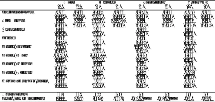
We re-run our estimates by type of school (middle or high school) for each labour-market indicator and by gender. The results appear in Tables 7 and 8. For men, practising team sports once more per week while in high school is associated with an increase in the hourly wage thirteen years later by 1.5%, the probability of being a manager by 2%, the probability of always having the freedom to make important decision at work by 1%, and the probability of being extremely satisfied at work by 0.8%. As suggested above, the op-portunity cost of time is likely higher in high school than in middle school. Older schoolboys who take the time to invest more in team sports system-atically enjoy labour market success as adults. There are some analogous effects for individual sports for boys in middle school in wave I: practising an individual sport one more per week is associated with an increase in the probability to be manager by 1.6%, a greater probability to be always free to make important decision at work (1%), but a smaller probability of being extremely satisfied at work (0.8%).

There is overall less evidence of a correlation between sport participation at school and labour-market outcomes for women. However, the distinc-tion according to when the sport was practised is much sharper: only sport in high school matters, and only two outcomes (being a manager and the

freedom to make important decisions).13 _{The marginal effect of practising}

13_{That sport seems to matter much more in high than in middle school provides some}

(17)

individual sport one more per week here is 2% for the probability of being a manager and 1.1% for being always free to make important decisions at work. Women’s labour-market outcomes then depend on investment in individ-ual sports, whereas for men team sports matter. This might be thought of as some a priori evidence that firms do not value the same skills for men and women. One interpretation is that firms value sports for its ability to “correct” natural inclination: women are already cooperative and know how to work in teams, while men are less collectively-minded.

Further Results

As the above results were the most significant for sporting activity during high school, the remaining results consider only this sub-sample.

A first check is to see whether there is any evidence that the effect of sport is non-linear. We therefore re-estimated equation (1) with dummy variables for each separate sport frequency. The findings (available on request) did not produce any particular insights.

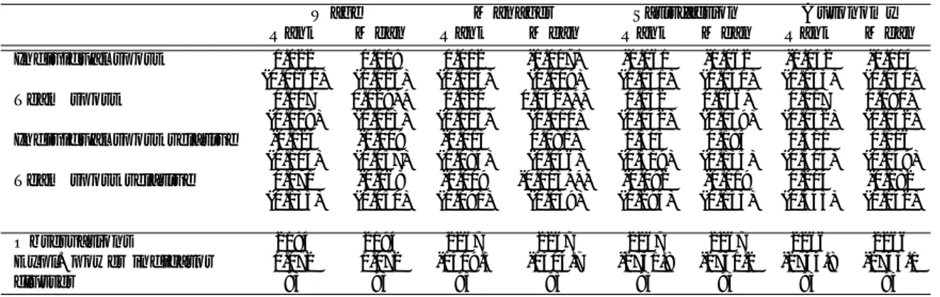
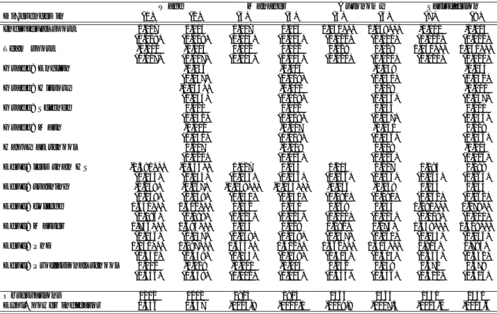
A perhaps more pertinent question is the role of relative versus absolute sport practice: the results are presented in Table 9 for men and Table 10 for women. For men, none of the measures of relative sports are significant (with the exception of the probability of being a manager) while the esti-mated coefficients on the absolute sport variables are positive and significant in about half of the regressions. The pattern is somewhat similar for women. Overall, we infer that sport participation in school is mostly not a zero-sum game. Irrespective of what schoolmates did, children’s own sport participa-tion while at high school is mostly positively rewarded on the labour market thirteen years later. This finding might be thought to cast some doubt on

the existence of "second-degree" signalling14 _{or a reputation effect. As with}

all work on social comparisons, however, this conclusion is subject to our having correctly identified the reference group. It is possible that firms to indeed compare candidates in terms of proxies for cognitive skills, but that we do not have good information on the references group.

sport and be successful on the labour market. As these factors are likely fixed over time, it should not matter at which age we observe the sporting activity.

(18)

Unobservable Heterogeneity

Our first pass at this, as mentioned above, is to add variables reflecting child behavior and ability from Wave I. Unfortunately, this seriously reduces our sample size, making it difficult to compare the results here to those listed in previous tables. The comparison is therefore carried out between the new estimations and previous specifications, run only on individuals for whom all of the relevant variables are available. The results for men appear in Table 11.

We find that the estimated coefficients on team sport practice remain positive, but are significant only for one labour-market outcome, being a manager. In general they are notably similar in size between the baseline specifications (given in the second column for each dependent variable) and regressions which control for individual ability, happiness at school and pop-ularity. Among these new control variables, grades play a significant role. However, the fact that the estimated coefficient on sport does not move much when we control for grades suggest that these measures of sport participation and academic achievement are largely independent of each other. The fact that the estimated sport coefficients here differ from those in the main tables then reflects the much smaller sample size in these new estimations.

For the sub-sample of women for whom the relevant information is avail-able, Table 12 shows that sport has no significant effect on labour-market outcomes, although again we should underline that very few observations can be used in this estimation. Nonetheless, it is worth noting the impact of the popularity variable on labour-market outcomes.

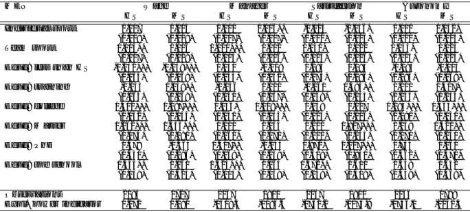
Last, we consider the differences in labour market outcomes between sib-lings. The results appear in Table 13. We do not carry out these estimations separately by gender, nor by school type (middle school or high school), due to sample size issues. We do control for gender and school type in wave I in the pooled regressions, however. The results here continue to show a result for sport at school for half of the labour market outcomes: even keeping the family environment constant (opportunities, human capital, etc.) those who practise more sport at school do better as adults on the labour market in terms of freedom to make decisions (individual sport) and job satisfaction (team sports).

For the other two labour market outcomes, being a manager and hourly wage, we find no significant correlations in the within-sibling sample. This is

(19)

in contrast to the baseline results in Tables 5 and 6. The variation in these two labour market outcomes (with respect to sport participation) is therefore between families rather than within family. As such, the probability of being a manager could reflect the role of family firms, or family influence within a firm. More generally it could reflect some aspect of upbringing that is shared by all children within the family (such as being encouraged to take decisions for themselves). The same kind of explanation can be advanced for the hourly wage. Children who were raised in a privileged socioeconomic environment will earn higher salaries than others; they may also have better opportunities to practise sport when at school. In this case, the correlation that we observe between adult wages and childhood sport is not causal, but rather reflects some hidden common factor at the family level.

5 Conclusion

This paper has used long-run American panel data to show that childhood sporting activities are correlated with adult labour market outcomes. Our data allows us to determine the impact of sport participation on four differ-ent measures of job quality separately by gender. We can also distinguish between the effect of individual and team sports. We make a number of attempts to address the issue of the endogeneity of sporting activities, via school fixed effects, controls for childhood behaviour and popularity, and within-sibling estimation. We continue to find significant correlations be-tween sport, especially when practised at high school, and a number of adult labour-market outcomes measured thirteen years later.

The marginal effect of sporting activity appears to be substantial. An in-crease in team sports at high school of once per week inin-creases adult hourly wage by 1.5% and the probability to be manager by 2%. The analogous effect on always being free to make important decisions at work is 1% and on the probability of being extremely satisfied at work is 0.8%. For girls, we identify marginal effects of the same magnitude with respect to being a manager and decision freedom, but with respect to individual sports.

Childhood sporting activities arguably help to foster human capital ac-cumulation via non-cognitive skills. The fact that different types of sports “work” to this extent for men and women suggests that different types of skill

(20)

matter across genders.

We test for the role of absolute compared to relative sport practice (com-pared to ones schoolmates), and find that only the former counts. As such, sport participation does not seem to be a zero-sum game, in the sense that greater participation for all would lead to better quality jobs for all (if we believe the causal link).

The impact of sport at high school is greater than that at middle school. As such, either sport has a greater skill return for older children, or that the signalling role of sport is more emphatic amongst older children who have many other potential uses of their time to hand. Alternatively, the network effect of sport participation may be much more relevant (in terms of labour market outcomes) at high school than at middle school.

We have attempted to deal with the endogenous choice of sporting ac-tivity. Our various controls and specification tests do knock out some of the effect of sport, but not all of it. It can always be countered that we have not adequately identified the variable that predicts both sport and labour mar-ket outcomes. However, we have considered this correlation within schools, within families, and controlling for child ability and personality. While there is still undoubtedly much to be learned about human-capital acquisition and labour-market success, the results here are consistent with at least some of the effect of school sport on subsequent labour market outcomes being causal.

(21)

References

Ashenfelter, Orley, & Krueger, Alan. 1994. Estimates of the economic return to schooling from a new sample of twins. The American Economic Review, 84(5), 1157–1173.

Ashenfelter, Orley, & Zimmerman, David. 1997. Estimates of the returns to schooling from sibling data: fathers, sons and brothers. The Review of Economics and Statistics, 79(1), 1–9.

Barron, John M., Ewing, Bradley T., & Waddell, Glen R. 2000. The Effects of High School Athletic Participation on Education and Labor Market Out-comes. Review of Economics and Statistics, 82, 409–421.

Bronars, Stephen G., & Oettinger, Gerald S. 2006. Estimates of the return to schooling and ability: evidence from sibling data. Labour Economics, 13, 19–34.

Cornelißen, Thomas, & Pfeifer, Christian. 2010. The Impact of Participa-tion in Sports on EducaParticipa-tional Attainment: New Evidence from Germany. Economics of Education Review, 29(1), 94–103.

Eber, Nicolas. 2002. La pratique sportive comme facteur de capital humain. Revue juridique et économique du sport, 65, 55–68.

Ewing, Bradley T. 1998. Athletes and Work. Economics Letters, 59, 113–117. Heckman, James J., & Rubinstein, Yona. 2001. The Importance of Noncog-nitive Skills: Lessons from the GED Program. The American Economic Review, 91(2), 145–149.

Humphreys, Brad, & Ruseski, Jane. Tech. rept. University of Alberta Work-ing Paper.

Kosteas, Vasilios D. 2010. British Journal of Industrial Relations, 49(1), 181–206.

Lechner, Michael. 2009. Long-run labour market and health effects of indi-vidual sports activities. Journal of Health Economics, 28(4), 839–854.

(22)

Levy-Garboua, Louis, Loheac, Youenn, & Fayolle, Bertrand. 2006. Prefer-ence Formation, School Dissatisfaction and Risky Behavior of Adolescents. Journal of Economic Psychology, 27(1), 165–183.

Long, James E., & Caudill, Steven B. 1991. The impact of Participation in Intercollegiate Athletics on Income and Graduation. Review of Economics and Statistics, 73, 525–531.

Rees, Daniel, & Sabia, Joseph. 2010. Sports participation and academic per-formance: Evidence from the National Study of Adolescent Health. Eco-nomics of Education Review, 29(5), 751–759.

Rooth, Dan Olof. 2011. Work Out or Out of Work: The Labor Market Return to Physical Fitness and Leisure Sport Activities. Labour Economics, 18(3), 399–409.

Spence, James. 1973. Job Market Signaling. Quarterly Journal of Economics, 87, 355–374.

(23)

Tables

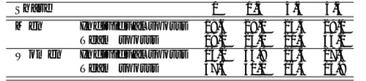
Table 1: Sport participation frequency by type of sport and gender.

Share 0 1.5 3.5 5.5

Men Individual sports 18.6 29.0 23.4 29.0

Team sports 19.2 25.1 21.5 34.2

Women Individual sports 13.2 33.9 25.4 27.5

Team sports 37.6 30.1 16.5 15.8

Table 2: Sport participation frequency by type of sport and school grade in Wave I.

Share 0 1.5 3.5 5.5

Middle school Individual sports 13.0 30.3 25.8 30.9

Team sports 20.2 27.8 21.7 30.3

High school Individual sports 17.9 32.3 23.6 26.2

(24)

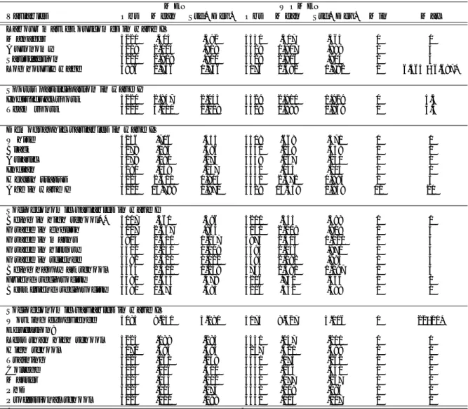
Table 3: Sample, summary statistics.

MEN WOMEN

Variables Obs Mean Std. Dev. Obs Mean Std. Dev. Min Max

Labour market outcomes in wave IV

Manager 5221 .414 .492 5330 .317 .465 0 1

Autonomy 5219 2.025 .918 5329 1.907 .899 0 3

Satisfaction 5221 2.918 .900 5328 2.906 .904 0 4

Log hourly wage 4996 2.756 0.746 5076 2.582 0.792 0 6.465 – 6.687*

Sports participation in wave I

Individual sport 5220 2.847 2.043 5329 2.910 1.929 0 5.5

Team sport 5221 3.010 2.118 5329 1.898 1.969 0 5.5

Demographic variables in wave IV

White 4236 .706 .455 4508 .668 .471 0 1 Black 4279 .194 .396 4541 .258 .438 0 1 Asiatic 4279 .081 .274 4539 .067 .250 0 1 Indian 4280 .059 .237 4542 .044 .205 0 1 Health status 5223 2.311 0.904 5331 2.372 0.883 1 5 Age in wave I 5220 15.789 1.870 5328 15.559 1.838 11 21

Socioeconomic variables in wave I

Being in high school** 5107 .561 .496 5210 .544 .498 0 1

Grade in english 5007 2.367 .964 5130 2.009 .918 1 4

Grade in maths 4804 2.410 1.047 4875 2.303 1.021 1 4

Grade in history 4502 2.230 1.019 4593 2.036 .971 1 4

Grade in science 4482 2.320 1.022 4594 2.092 .985 1 4

Being happy at school 3364 2.400 1.249 3733 2.491 1.197 1 5

Friend reciprocity 3380 0.644 .479 4216 .732 .443 0 1

Best friend reciprocity 3380 0.374 .484 4216 .452 .498 0 1

Socioeconomic variables in wave IV

Working experience 5083 9.231 3.080 5075 8.627 3.006 0 22–21*

Education:

Less than high school 5223 .088 .283 5331 .047 .211 0 1

High school 5171 .583 .493 5257 .521 .499 0 1 Training 5223 .060 .238 5331 .074 .262 0 1 College 5223 .216 .412 5331 .264 .441 0 1 Master 5223 .043 .202 5331 .077 .267 0 1 PhD 5223 .005 .074 5331 .009 .096 0 1 Professional school 5223 .010 .099 5331 .014 .117 0 1

*Minimum and maximum are the same for men and women, except for the log hourly wage and the number of years of working experience. In these two cases, the first figure concerns men, the second refers to women.

(25)

Table 4: Significant difference in the mean between the sporty sample and the non-sporty sample.

Sport less than Sport 3 or more signif var if 3 or more

Variables 3 times weekly times weekly times weekly

Labour market outcomes in wave IV

Log hourly wage 2.44 2.56 *** 4.9%

Autonomy 1.82 1.94 *** 6.6%

Manager 0.34 0.39 *** 14.7%

Satisfaction 2.85 2.86 0.4%

Working 0.77 0.8 *** 3.9%

Working experience 8.9 8.39 *** -5.7%

Demographic variables in wave IV

Woman 0.59 0.45 *** -23.7% Black 0.22 0.24 ** 9.1% Asian 0.08 0.07 -12.5% Indian 0.06 0.05 * -16.7% White 0.68 0.68 *** 0.0% Age 28.68 28.29 *** -1.4% Health status 2.39 2.3 *** -3.8%

Socioeconomics variables in wave I

In high school in W1 0.58 0.48 *** -17.2% Best friend 0.43 0.4 ** -7.0% Friend 0.7 0.68 ** -2.9% Grade in Math 2.39 2.28 *** -4.6% Grade in History 2.17 2.1 *** -3.2% Grade in Science 2.22 2.16 *** -2.7% Grade in English 2.19 2.14 *** -2.3%

Being happy at school 2.5 2.34 *** -6.4%

Socioeconomic variables in wave IV

Less than high school 0.08 0.08 0.0%

High school 0.56 0.54 *** -3.6% Training 0.07 0.06 ** -14.3% College 0.22 0.24 *** 9.1% Master 0.05 0.06 *** 20.0% PhD 0.01 0.01 0.0% Professional school 0.01 0.01 *** 0.0%

(26)

Table 5: Results by labour market outcome: Men sample.

Wage Manager Satisfaction Autonomy

Individual sport 0.005 0.007 -0.032* 0.020 (0.006) (0.005) (0.017) (0.015) Team sport 0.012** 0.012*** 0.034* 0.033** (0.005) (0.004) (0.018) (0.016) Black -0.205*** -0.111*** -0.456*** -0.095 (0.034) (0.021) (0.077) (0.074) Asian 0.133*** -0.004 -0.096 0.027 (0.035) (0.034) (0.089) (0.074) Indian -0.063 -0.045 -0.163 -0.145 (0.058) (0.029) (0.104) (0.111) Health status -0.045*** -0.006 -0.255*** -0.122*** (0.010) (0.009) (0.042) (0.033) Age2 _0.000*** _-0.000* _0.000 _-0.001* (0.000) (0.000) (0.000) (0.000) Working exp 0.007 0.022*** 0.023 0.065*** (0.006) (0.004) (0.014) (0.012)

Educ: less than HS -0.270*** 0.016 0.177 -0.115

(0.047) (0.025) (0.115) (0.136) Educ: training 0.016 -0.030 0.110 0.211* (0.050) (0.032) (0.129) (0.124) Educ college 0.305*** 0.079*** 0.093 0.409*** (0.026) (0.022) (0.081) (0.077) Educ: Master 0.304*** 0.023 0.454*** 0.248* (0.057) (0.046) (0.155) (0.139) Educ: PhD 0.139 0.279** 1.170** 0.518* (0.282) (0.117) (0.475) (0.309)

Educ: Professional school 0.281* 0.271*** 0.571* 0.632*

(0.148) (0.088) (0.332) (0.360) Constant (cut 1) 2.267*** -0.172** -4.251*** -2.805*** (0.110) (0.084) (0.331) (0.272) Cut 2 -2.874*** -0.961*** (0.308) (0.285) Cut 3 -1.397*** 0.526* (0.306) (0.293) Cut 4 0.843*** (0.305) Observations 4006 4157 4156 4154

Explanation power indicator 0.084 -2765.9 -5049.2 -5096.7

Robust standard errors in parentheses

* significant at 10%; ** significant at 5%; *** significant at 1%

Explanation power indicator is respectively: the R-squared, the log likelihood and the log pseudo-likelihood.

(27)

Table 6: Results by labour market outcome: Women sample.

Individual sport -0.001 0.013*** 0.011 0.043** (0.005) (0.004) (0.016) (0.019) Team sport -0.002 0.002 -0.003 0.018 (0.006) (0.004) (0.017) (0.017) Black -0.063** -0.038** -0.526*** -0.048 (0.029) (0.017) (0.070) (0.072) Asian 0.279*** -0.004 -0.257*** -0.118 (0.050) (0.018) (0.098) (0.108) Indian 0.006 0.012 -0.160 0.025 (0.064) (0.032) (0.131) (0.156) Health status -0.087*** 0.005 -0.232*** -0.133*** (0.014) (0.007) (0.039) (0.038) Age2 _0.001*** _0.000 _0.001** _0.000 (0.000) (0.000) (0.000) (0.000) Working exp -0.009* 0.009*** 0.008 0.022 (0.006) (0.003) (0.013) (0.015)

Educ: less than HS -0.372*** -0.042 -0.294** -0.288

(0.069) (0.043) (0.126) (0.183) Educ: training -0.033 -0.081** 0.160 0.049 (0.046) (0.032) (0.134) (0.111) Educ: college 0.345*** 0.039* 0.036 0.077 (0.039) (0.023) (0.094) (0.078) Educ: Master 0.450*** 0.009 0.121 0.070 (0.040) (0.034) (0.146) (0.114) Educ: PhD 0.418** 0.287*** 0.148 1.008*** (0.183) (0.078) (0.292) (0.349)

Educ: Professional school 0.389** 0.274*** -0.001 -0.082

(0.155) (0.061) (0.251) (0.208) Constant (cut 1) 2.210*** -0.364*** -4.064*** -2.534*** (0.126) (0.073) (0.283) (0.332) Cut 2 -2.527*** -0.425 (0.258) (0.329) Cut 3 -1.156*** 1.154*** (0.257) (0.325) Cut 4 1.132*** (0.264) Observations 4121 4314 4314 4314

Explanation power indicator 0.126 -2670.3 -5226.4 -5336.3

(28)

Table 7: Labour market outcomes by school type: Men.

MEN Wage Manager Satisfaction Autonomy

HS MS HS MS HS MS HS MS

Individual sport 0.007 0.005 0.000 0.016** -0.023 -0.046* 0.010 0.042*

(0.008) (0.009) (0.007) (0.007) (0.022) (0.026) (0.020) (0.024)

Team sport 0.015** 0.006 0.020*** 0.002 0.041* 0.022 0.043* 0.025

(0.007) (0.008) (0.005) (0.006) (0.025) (0.026) (0.024) (0.024)

Educ: less than HS -0.232*** -0.259*** 0.050 -0.019 0.284 0.184 -0.193 -0.103

(0.064) (0.068) (0.043) (0.042) (0.173) (0.186) (0.295) (0.169) Educ: training -0.053 0.139** -0.046 0.011 -0.160 0.484** 0.101 0.417* (0.065) (0.068) (0.040) (0.057) (0.159) (0.233) (0.144) (0.234) Educ: college 0.302*** 0.287*** 0.056* 0.109*** 0.048 0.127 0.294*** 0.564*** (0.032) (0.044) (0.031) (0.033) (0.125) (0.116) (0.091) (0.130) Educ: Master 0.262*** 0.335*** 0.000 0.054 0.201 0.827*** 0.049 0.521** (0.074) (0.081) (0.061) (0.071) (0.201) (0.233) (0.170) (0.240) Educ: PhD 0.379 -0.464 0.417** -0.155 0.972* 2.227*** 0.743 0.061 (0.350) (0.296) (0.169) (0.238) (0.518) (0.831) (0.462) (0.370)

Educ: spe school 0.335** 0.060 0.325*** 0.064 0.572** 0.600 0.538 0.652

(0.159) (0.325) (0.104) (0.159) (0.258) (1.409) (0.449) (0.468)

Observations 2194 1727 2267 1801 2267 1800 2266 1799

Expl. power indicator 0.072 0.081 -1509.3 -1186.4 -2752.2 -2174.8 -2746.0 -2232.3

(29)

Table 8: Labour market outcomes by school type: Women.

WOMEN Wage Manager Satisfaction Autonomy

HS MS HS MS HS MS HS MS

Individual sport 0.000 -0.002 0.020*** 0.005 0.017 0.004 0.054* 0.027

(0.009) (0.008) (0.006) (0.005) (0.020) (0.024) (0.028) (0.023)

Team sport -0.000 -0.003 0.007 -0.003 -0.016 0.009 0.024 0.015

(0.008) (0.009) (0.006) (0.006) (0.022) (0.025) (0.023) (0.023)

Educ: less than HS -0.270** -0.410*** -0.071 -0.022 0.090 -0.559*** -0.092 -0.444*

(0.119) (0.088) (0.053) (0.062) (0.194) (0.205) (0.321) (0.254) Educ: training -0.090 0.021 -0.064 -0.108** 0.020 0.292 -0.018 0.074 (0.079) (0.057) (0.040) (0.048) (0.182) (0.201) (0.145) (0.170) Educ: college 0.308*** 0.359*** 0.058** 0.009 0.114 -0.057 0.164* -0.034 (0.049) (0.050) (0.029) (0.033) (0.118) (0.128) (0.093) (0.126) Educ: Master 0.455*** 0.383*** 0.045 -0.048 0.188 0.013 0.068 0.111 (0.044) (0.061) (0.045) (0.051) (0.177) (0.257) (0.159) (0.162) Educ: PhD 0.325 0.563*** 0.271*** 0.363*** 0.091 0.357 1.054** 1.005* (0.230) (0.159) (0.101) (0.131) (0.373) (0.391) (0.428) (0.593)

Educ: Professional school 0.493*** 0.085 0.337*** 0.169* -0.107 0.363 0.012 -0.271

(0.168) (0.237) (0.077) (0.096) (0.307) (0.398) (0.233) (0.514)

Observations 2201 1837 2288 1936 2287 1937 2288 1936

Table 9: Absolute or relative sports? Boys attending high school in Wave I.

Rank Mean Rank Mean Rank Mean Rank Mean

Individual sport 0.022 0.009 0.002 -0.017* -0.061 -0.062 -0.042 -0.014

(0.0161) (0.015) (0.013) (0.009) (0.051) (0.040) (0.043) (0.040)

Team sport 0.007 0.029** 0.021 0.042*** 0.052 0.066* 0.017 0.080*

(0.019) (0.013) (0.013) (0.010) (0.042) (0.039) (0.052) (0.042)

Individual sport relative -0.124 -0.009 -0.013 0.081* 0.305 0.185 0.411 0.116

(0.104) (0.057) (0.084) (0.046) (0.319) (0.135) (0.304) (0.149)

Team sport relative 0.071 -0.068 -0.009 -0.105*** -0.092 -0.119 0.204 -0.182

(0.135) (0.050) (0.091) (0.039) (0.294) (0.153) (0.345) (0.142)

Observations 2194 2194 2267 2267 2267 2267 2266 2266

cluster 93 93 93 93 93 93 93 93

(30)

Table 10: Absolute or relative sports? Girls attending high school in Wave I.

Manager Autonomy

Rank Mean Rank Mean

Individual sport 0.035*** 0.028** 0.113** -0.007

(0.014) (0.011) (0.055) (0.049)

Team sport 0.017* 0.020** 0.037 0.017

(0.010) (0.008) (0.038) (0.033) Individual sport relative -0.118 -0.037 -0.445 0.269* (0.091) (0.039) (0.321) (0.154)

Team sport relative -0.107 -0.066** -0.138 0.0322

(0.076) (0.030) (0.284) (0.117)

Observations 2288 2288 2288 2288

Expl. power indicator -1426.6 -1426.4 -2715.5 -2716.8 Robust standard errors in parentheses

* significant at 10%; ** significant at 5%; *** significant at 1% Explanation power indicator is respectively: the R-squared, the log likelihood and the log pseudo-likelihood.

Table 11: Controlling for happiness at school, ability and popularity. Boys attending high school in wave I.

(1) (2) (3) (4) (5) (6) (7) (8) Individual sport -0.013 -0.014 -0.009 -0.010 -0.072* -0.064 -0.019 -0.015 (0.017) (0.017) (0.016) (0.016) (0.043) (0.043) (0.033) (0.033) Team sport 0.016 0.020 0.027** 0.029*** 0.015 0.017 0.050 0.047 (0.015) (0.014) (0.011) (0.011) (0.039) (0.038) (0.038) (0.039) Best friend 0.024 0.044 -0.210 0.143 (0.070) (0.049) (0.195) (0.194) Friend 0.030 0.004 0.213 0.091 (0.077) (0.054) (0.209) (0.182) Grade: English -0.018 0.033 -0.273*** -0.059 (0.027) (0.024) (0.088) (0.114) Grade: Math -0.071** -0.055*** -0.008 0.026 (0.027) (0.020) (0.097) (0.094) Grade: History -0.025 -0.023 0.008 -0.094 (0.029) (0.023) (0.097) (0.102) Grade: Science 0.011 -0.009 0.009 -0.017 (0.029) (0.026) (0.103) (0.089)

Happy at school (scale) 0.000 0.011 -0.074 -0.038

(0.020) (0.019) (0.059) (0.057)

Observations 667 667 689 689 693 693 693 693

Expl. power indicator 0.112 0.098 -457.9 -463.7 -830.2*XXX -837.2*XXX -814.3 -817.2

(31)

Table 12: Controlling for happiness at school, ability and popularity. Girls attending high school in wave I.

Manager Autonomy (1) (2) (3) (4) Individual sport 0.015 0.015 0.040 0.036 (0.011) (0.011) (0.044) (0.044) Team sport 0.000 0.000 0.027 0.034 (0.011) (0.011) (0.047) (0.046) Best friend 0.041 0.328** (0.047) (0.164) Friend -0.091* 0.005 (0.054) (0.177) Grade: English -0.001 0.187 (0.027) (0.126) Grade: Math -0.010 0.006 (0.021) (0.081) Grade: History 0.012 0.004 (0.024) (0.145) Grade: Science 0.009 -0.056 (0.021) (0.090)

Happy at school (scale) -0.017 -0.091

(0.017) (0.069)

Observations 728 728 728 728

Expl. power indicator -457.5 -459.8 -866.9 -872.4 Robust standard errors in parentheses

* significant at 10%; ** significant at 5%; *** significant at 1% Explanation power indicator is respectively: the R-squared, the log likelihood and the log pseudo-likelihood.

(32)

Table 13: Siblings sample.

Wage Manager Autonomy Satisfaction

Differences in (1) (2) (3) (4) (5) (6) (7) (8) Individual sport 0.007 0.004 0.007 0.006 0.060*** 0.059*** -0.001 -0.003 (0.018) (0.018) (0.005) (0.005) (0.022) (0.022) (0.022) (0.022) Team sport -0.002 -0.003 0.002 0.002 0.029 0.029 0.051*** 0.051*** (0.017) (0.017) (0.004) (0.004) (0.020) (0.020) (0.020) (0.020) Grade: English -0.036 -0.005 -0.048 -0.033 (0.037) (0.009) (0.040) (0.042) Grade: History -0.065** -0.001 0.008 -0.000 (0.033) (0.008) (0.035) (0.037) Grade: Science 0.020 0.002 0.054 0.010 (0.031) (0.008) (0.037) (0.035) Grade: Math -0.012 -0.007 -0.040 0.019 (0.030) (0.008) (0.036) (0.036) Happy at school 0.007 -0.009 0.009 -0.013 (0.021) (0.006) (0.026) (0.026)

Educ: less than HS -0.381*** -0.354** 0.027 0.033 0.204 0.217 0.194 0.199

(0.144) (0.145) (0.035) (0.036) (0.166) (0.166) (0.163) (0.165) Educ: training -0.248* -0.267* -0.148*** -0.153*** -0.046 -0.059 0.154 0.154 (0.138) (0.138) (0.050) (0.050) (0.190) (0.191) (0.162) (0.162) Educ: college 0.640*** 0.602*** 0.032 0.030 0.068 0.045 0.281*** 0.279** (0.086) (0.088) (0.024) (0.025) (0.110) (0.113) (0.108) (0.110) Educ: Master 0.736*** 0.683*** 0.035 0.028 0.282* 0.273* 0.438*** 0.429*** (0.156) (0.157) (0.038) (0.039) (0.157) (0.161) (0.153) (0.156) Educ: PhD 1.140*** 1.087*** 0.335** 0.312** 1.362*** 1.314*** 0.805* 0.783* (0.341) (0.338) (0.154) (0.158) (0.314) (0.315) (0.445) (0.452)

Educ: Professional school 0.002 -0.029 -0.001 -0.003 0.142 0.149 0.572 0.579

(0.536) (0.538) (0.102) (0.105) (0.435) (0.436) (0.422) (0.426)

Observations 1202 1202 1823 1823 1565 1565 1551 1551