HAL Id: halshs-00255794
https://halshs.archives-ouvertes.fr/halshs-00255794
Submitted on 14 Feb 2008HAL is a multi-disciplinary open access archive for the deposit and dissemination of sci-entific research documents, whether they are pub-lished or not. The documents may come from
L’archive ouverte pluridisciplinaire HAL, est destinée au dépôt et à la diffusion de documents scientifiques de niveau recherche, publiés ou non, émanant des établissements d’enseignement et de
Optimum income taxation and layoff taxes
Pierre Cahuc, André Zylberberg
To cite this version:
Pierre Cahuc, André Zylberberg. Optimum income taxation and layoff taxes. Journal of Public Eco-nomics, Elsevier, 2008, 92 (10-11), pp.2003-2019. �10.1016/j.jpubeco.2007.12.006�. �halshs-00255794�
Optimum Income Taxation and Layo¤ Taxes
¤
Pierre Cahuc
yCREST-INSEE, Université Paris 1, CEPR, IZA.
André Zylberberg
EUREQua-Université Paris 1 and CNRS
July 2005 (…rst version: June 2004)
Abstract
This paper analyzes optimum income taxation in a model with endogenous job destruc-tion that gives rise to unemployment. It is shown that optimal tax schemes comprise both payroll and layo¤ taxes when the state provides public unemployment insurance and aims at redistributing income. The optimal layo¤ tax is equal to the social cost of job destruction, which amounts to the discounted value of the sum of unemployment bene…ts (that the state pays to unemployed workers) and payroll taxes (that the state does not get when workers are unemployed). Our quantitative analysis suggests that the introduction of layo¤ taxes, that are usually absent from actual tax schemes, could lead to signi…cant increases in employment and GDP.
Keywords: Layo¤ taxes, Optimal taxation, Job destruction. JEL codes: H21, H32, J38, J65
¤We wish to thank, without implication, Guy Laroque and Bernard Salanié for very helpful comments. We
also thank participants in seminars at CREST, Université de Paris 1, Université d’Aix-Marseille 2, Norwegian School of Economics and Business Administration and CERGE.
yCorresponding author: CREST-INSEE, Timbre J 360, 15, Boulevard Gabriel-Peri, 92245, Malako¤, France.
1 Introduction
So far, the in‡uence of taxes on job creation and destruction has been neglected to a large extent by the economics of taxation (see Salanié, 2003, for a recent survey). Yet, many empirical studies have shown that modern economies face dramatic job turnover that in‡uences employment and growth. From this point of view it is important to analyze the impact of taxes on job creation and destruction. In a seminal paper, Feldstein (1976) argued that payroll taxes used to …nance unemployment bene…ts in most OECD countries induce too many layo¤s, because employers do not take into account the cost of insurance provided by the state to the unemployed workers. To avoid this excess of job destruction unemployment insurance has to be …nanced by layo¤ taxes. The experience rating system used in the United States is an example of layo¤ taxes that induce …rms to internalize the cost associated with their layo¤ decisions (Burdett and Wright, 1989a, b, Anderson and Meyer, 1993, 2000, Blanchard and Tirole, 2004, Cahuc and Malherbet, 2004).
In this paper, it is argued that layo¤ taxes are not only a natural counterpart to the state provision of unemployment bene…ts: they are also a natural counterpart to other public expen-ditures. Indeed, when employers destroy a job, they do not take into account that workers who are …red will continue to consume collective goods but may contribute to a much smaller extent to …nance these goods. In this context, if individuals bring less in the budget of the state when they are unemployed than when they are employed, the social value of jobs, that is their value for the entire society, is larger than their private value, that is their value for the worker and the employer. This phenomenon can lead to excessive job destruction in the absence of layo¤ taxes. Therefore, layo¤ taxes should not be only a part of the unemployment insurance system. They should also be integrated as an instrument in the overall tax system used to …nance public expenditures.
which analyzes the tax-subsidy schemes that implement second-best allocations when the state has incomplete information about the preferences of individuals. More precisely, we follow the approach of Diamond (1980) in which individuals, whose only decision is whether to work or not, di¤er in their taste for leisure as well in ability (see also: Beaudry and Blackorby, 1997, Choné and Laroque, 2005, Laroque, 2005, Saez, 2002). In Diamond’s model, the ability of employees, which determines the market income and then the level of taxes, is observable, but taste for leisure is private information. In our paper, Diamond’s model is enriched in order to account for unemployment and job destruction. It is assumed that the productivity of each job depends on the ability of the worker, that is common knowledge only when he participates in the labor market, and a random job speci…c productivity shock, that is privately known by the …rm and the worker once the worker has been recruited. Moreover, …rms are risk neutral, workers are risk averse and it is assumed that unemployment insurance is provided by the state.1 In this context, some workers who have decided to participate in the labor market are unemployed because jobs whose productivity is too low are destroyed.
Our paper analyzes the optimal tax-subsidy schemes that implement second-best allocations when there is job destruction. The main result is that optimal tax schemes comprise both payroll and layo¤ taxes when the state provides public unemployment insurance and aims at redistributing income. It turns out that the optimal layo¤ tax is equal to the social cost of job destruction, which amounts to the discounted value of the sum of the unemployment bene…ts (that the state pays to unemployed workers) and payroll taxes (that the state does not get when
1The “implicit contract literature” has shown that risk neutral …rms fully insure workers against income
‡uctuations by giving constant wages to the employees and unemployment bene…ts to the workers they layo¤ (Baily, 1974, Azariadis, 1975, Rosen 1985, Pissarides, 2001), However, in the real world, unemployment insurance is not provided by …rms. Some rare exceptions are presented and discussed by Chui and Karni (1998) who stressed that the failure of the private sector to provide unemployment insurance can be explained by the interaction of adverse selection and moral hazard problems: an isolated …rm that would o¤er private insurance would attract workers with strong work aversion, who would try to be …red as soon as they become eligible to the unemployment bene…ts. If work aversions are not observable and the level of e¤ort of the employees not veri…able, it can be the case that private unemployment insurance cannot emerge. In our paper, we assume, like Burdett and Wright (1989a,b) and Blanchard and Tirole (2004) among many others, that unemployment insurance is provided by the state.
workers are unemployed).
This result is obtained in two steps. In the …rst step, we consider a static framework which allows us to get a set of intermediary results. More precisely, if the state does not aim at redis-tributing income across individuals with di¤erent abilities, it is shown that …rst-best allocations can be reached thanks to unemployment bene…ts that are entirely …nanced by layo¤ taxes. This is a simple generalization of the result obtained by Blanchard and Tirole (2004) in a model without participation decision and heterogeneity of workers. If the state aims at redistributing income across individuals with di¤erent abilities, …rst-best allocations cannot be reached because the taste for leisure is private information. In that case, it is shown that second-best allocations are obtained thanks to tax-subsidy schemes that comprise layo¤ taxes equal to the sum of the unemployment bene…ts and the payroll tax raised on the production of the employees.
Then, in the second step, the properties of optimal tax-subsidy schemes are derived in a dynamic version of the static model. This dynamic version is useful to give quantitative insights on the optimal amount of layo¤ taxes and on their impact on employment, unemployment, GDP, welfare and the budget of the state.
The paper is organized as follows. The preferences, the technology and the …rst-best allo-cations of the static benchmark economy are presented in section 2. Section 3 is devoted to the analysis of the tax-subsidy schemes that allow the state to reach second-best allocations. Section 4 provides a dynamic extension of the benchmark model. The dynamic model is utilized to yield quantitative evaluations of the impact of layo¤ taxes in section 5. Section 6 concludes.
2 The Benchmark Model
2.1 Preferences and technology
We consider a static economy with a continuum of individuals whose size is normalized to one. There are two goods: labor and a marketable good produced thanks to labor. Individuals outside
the labor force do not produce the marketable good. Individuals inside the labor force can be either employed or unemployed.
An individual is described by a set of exogenous characteristics, denoted by s = (y; z); where ystands for his ability and z for his taste for leisure. We assume that (y; z) has a joint density h(y; z) with h > 0 over the support S½ [ymin; +1) £ R; h is continuous. The preferences of the type-s individual are represented by the utility function v(c + z`), twice derivable, increasing and strictly concave, where c ¸ 0 denotes consumption, ` 2 f0;1g denotes leisure that amounts to zero if the individuals is active (either employed or unemployed) and to one if he is not in the labor force. The set of inactive individuals is denoted by SI and the set of active agents (which comprises employed and unemployed workers) is denoted by SA:
Creating a job for a type-(y; z) individual entails a …xed cost denoted by k(y) > 0: When such an individual gets a job, he can produce x ¢ y units of the marketable good where x 2 R is an idiosyncratic shock drawn in a distribution with a continuous di¤erentiable cumulative distribution function denoted by G. Each individual can occupy at most one job.
An allocation de…nes the consumption and the employment status of all the agents of the economy. It is a mapping that associates to each type-s individual, conditional on the realization of the productivity shock x for active individuals, his consumption: c(s); if s 2 SI, c(s; x) if s2 SA; and his employment status: inactive (`(s) = 1), employed (`(s) = 0 and marketable production = x ¢ y) or unemployed (`(s) = 0 and marketable production = 0): The choice between employment and unemployment amounts to de…ne the set of values of the productivity parameter x; denoted by W (y) ½ R; for which the type-(y; z) individuals who belong to SA work.
All allocations have to satisfy the feasibility constraint: Z SA · Y (y)¡ Z Rc(y; z; x)dG(x) ¸ h(y; z)dydz = Z SI
c(y; z)h(y; z)dydz; (1)
ability y.
2.2 First-best allocations
First-best allocations are chosen by a fully informed planner who has complete information on the pair s = (y; z) describing each agent’s characteristics and on the productivity shocks x. First-best allocations are such that there are no other feasible allocations that can improve the welfare of at least one agent without worsening the welfare of the others. When an agent faces risky outcomes – this will be the case for the active agents –, it is assumed that feasible allocations are ranked according to the expected utility criterion conditional on characteristics (y; z). The time sequence of events that describes the decision of the planner runs as follows: 1) The planner decides which set of agents s 2 SIare inactive (`(s) = 1), and which set of agents s2 SA are allowed to participate in the production of the consumption good (`(s) = 0). The planner also announces the consumption of the marketable good of every type-s individuals. The consumption can be conditional on the realization of the productivity shocks for active individuals.
2) Every individual in SA makes a draw x from the cdf function G that raises his potential production to the level x ¢ y: After observing x; the planner decides whether each individual in SA actually produces or not (this is the job destruction decision). Individuals produce and consume according to the plan announced at step1).
The …rst-best allocations can be obtained by backward induction.
At step2), once x has been drawn, it is worthwhile keeping employed the individuals who produce more on-the-job than in unemployment, i.e. it is worthwhile keeping employed the type-(y; z) workers such that x¢ y ¸ 0. Therefore, the choice of the set of values of the productivity parameter x; denoted by W (y) ½ R; for which the type-(y;z) individuals who belong to SAwork, boils down to the choice of the reservation productivity below which the type-(y; z) individuals belonging to SAare unemployed. The …rst-best reservation productivity, denoted by X¤;satis…es
the productive e¢ciency condition:
X¤= 0: (2)
Since it costs k(y) to assign the type-(y; z) individual to SA, the average net …rst-best produc-tion of an individual with ability y belonging to SA amounts to Y¤(y) =¡k(y)+ yR0+1xdG(x): At step1) the planner has to choose the consumption of the marketable good for every indi-vidual. The consumption of inactive individuals can only depend on their type s. For the active individuals, the assumption of risk aversion implies that the certainty equivalent income of the lottery fc(s;x)g is smaller than the expected consumptionRRc(s; x)dG(x): Accordingly, a social planner whose decisions are based upon the expected utility criterion can always save resources by providing to the type-s individuals belonging to SA the certainty equivalent associated with the lottery fc(s;x)g : It follows that the …rst-best allocations necessarily insure all individuals in SA against productivity shocks and give them the same consumption whether employed or unemployed.
At step1), the planner also chooses the set of individuals who participate in the labor market. It can easily be understood that the set SA of active agents only comprises type-s individuals such that Y¤(y) ¸ z: Imagine that we can …nd in SA an agent with Y¤(y) < z: This agent can get the same utility level when he is inactive if his consumption of the marketable good is decreased by z. This allows the social planner to win z and lose Y¤(y) as forgone production, which yields a positive net gain equal to z ¡ Y¤(y): Thus, it is not optimal to have an active individual whose taste for leisure is larger that his expected production. An analogous reasoning shows that the set SI comprises type-s individuals such that Y¤(y) < z. In other words, the participation decision reads:
`¤(y; z) = ½
0 if z · Y¤(y) =¡k(y) + yR+1
0 xdG(x)
1 otherwise. (3)
Proposition 1 A feasible allocation is a …rst-best allocation if and only if:
1. Active individuals are employed when x ¸ 0 and unemployed otherwise.
2. Every agent with the same type s belonging to the set SA of active individuals gets the same consumption level whatever the value of x:
3. The set SA of active individuals comprises all the type-s individuals such that Y¤(y)¸ z; and the set SI of inactive individuals comprises all the agents such that Y¤(y) < z:
Proof. see appendix A.
Claim 3 of proposition 1 is a particular case of a more general result established in Laroque (2005) stating that in an economy with labor supply choice at the extensive margin, where the agents choose whether to work or not to work, it is Pareto optimal that someone works if and only if his productivity is larger than the extra necessary income to compensate him for the hardship of work. In our economy, the agents are perfectly insured against unemployment risks and the extra necessary income to compensate an individual, with taste for leisure z, for being active is simply equal to z while his expected productivity amounts to Y¤(y):
3 Second-best allocations and optimal tax-subsidy schemes
This section is devoted to the design of optimal …scal policies in a framework in which the state is committed to a tax-subsidy scheme and where the marketable good is produced on a perfectly competitive market. Contrary to the …rst-best environment, the state does not observe the characteristics of the agents. Namely, the taste for leisure z always remains private information of the worker. The ability y and the idiosyncratic productivity shock x are observed by the …rm and the worker but are not veri…able. The distributions of x; y and z are common knowledge. The state only observes the labor contracts and whether individuals work. This implies that the state knows who has been …red and is able to distinguish unemployed workers from inactive
individuals. In this situation, the tax-subsidy scheme can only depend on the elements of the labor contracts and on the employment status (employed, unemployed, inactive).
First, the decentralized equilibrium is studied. Then, we analyze the optimal policies.
3.1 Decentralized equilibrium
The marketable good is produced by …rms on a competitive market with free entry. As the labor contracts only stipulate wages, the state can use tax-subsidy schemes conditional on three elements: 1) the wage, denoted by w; 2) the employment status (employed, unemployed or inactive); 3) the job destruction decision. Accordingly, the tax-subsidy scheme can comprise a payroll (or income) tax, ¿(w); a layo¤ tax, f(w); unemployment bene…ts b(w); and a income guarantee ½ paid to the inactive persons. In this framework, the overall consumption of the individual who has signed a labor contract that stipulates a wage w amounts to w if he is employed and to b(w) if he is unemployed. The type-(y; z) individual that does not participate in the labor market gets a utility level v(z +½). The wage w entails labor costs equal to w +¿(w) if workers remain employed and to f(w) if they are …red.
The time sequence of events runs as follows:
1) The state announces a balanced budget tax-subsidy scheme f¿(w); f(w);b(w);½g. 2) Individuals decide whether they belong to the labor force or stay inactive.2 3) Employers enter into Bertrand competition to hire workers.
4) The speci…c productivity shocks x occur and employers decide whether they keep the workers or they destroy the jobs. Then, employers pay the wage and the payroll tax for every continuing job. Every destroyed job gives rise to the payment of layo¤ taxes. Employed workers get a wage w, unemployed workers get unemployment bene…ts b(w) and inactive individuals get the garantee income ½:
2It is assumed that individuals who decide to belong to the labor force reveal their true productivity. If they
have the possibility to behave as agents of lower productivity without cost, thruthful revelation would only obtain under the condition that their wage w be non decreasing in y; a condition that will be satis…ed in equilibrium.
In this subsection, we characterize the existence and the properties of the competitive equi-librium of the labor market for the tax-subsidy scheme announced at step1). This problem can be solved by backward induction.
At step4) …rms destroy jobs if and only if their pro…ts, x ¢y¡ w¡ ¿(w); are lower than their destruction costs, ¡f(w): The job destruction decision boils down to the choice of a reservation value of the productivity parameter x; denoted by X(w; y); below which job are destroyed.3 The reservation productivity reads:
X (w; y) = [w + ¿(w)¡ f(w)] =y: (4)
For individuals with ability y; the job destruction rate (or equivalently the unemployment rate), denoted by q(w; y); is equal to G(X(w; y)):
At step3), the expected pro…t of an employer o¤ering a contract w to a type-(y; z) worker, denoted by J(w; y); reads:
J (w; y) =¡k(y) + Z +1
X(w;y)
[x¢ y ¡ w ¡ ¿(w)] dG(x) ¡ q(w; y)f (w) : (5)
Existence and unicity of the Bertrand equilibrium depend on the properties of the functions k(¢) and G(¢) and of the functions ¿(¢); b(¢); f(¢) describing the tax-subsidy schedule. We shall assume that all these functions are such that the expected pro…t J(w; y) satis…es the properties summarized in Assumption 1:
Assumption 1
1.i) 8y; fw ¸ 0 j J(w;y) = 0g 6= ;: 1.ii) 8y; limw!+1J(w; y) < 0:
3This behavior comes from the assumption that the reservation value of the productivity parameter x is not
contractable and that the …rm cannot commit ex-ante to this reservation value by keeping aside funds to be paid to a third party in case of layo¤. See the discussion in Blanchard and Tirole (2004).
Conditions 1.i) and 1.ii) are necessary and su¢cient conditions to obtain a unique Bertrand equilibrium with positive …nite wages.4 More precisely, condition 1.ii) prevents employers from o¤ering unbounded wages, thus Bertrand competition between the employers drives expected pro…ts to zero and condition 1.i) states that for any y there exists at least one positive wage giving an expected pro…t equal to zero. Then the Bertrand equilibrium wage is the highest value of w that solves the zero pro…t condition J(w; y) = 0: In other words, conditions 1.i) and 1.ii) imply that there exists a unique equilibrium wage contract w(y) o¤ered to the type-(y; z) workers, which reads:
w(y) = supfw ¸ 0g j J(w; y) = 0g: (6)
Furthermore, we can obtain a precise result concerning the monotonicity of the equilibrium wage function w(y) if we add the following (reasonable) assumption.
Assumption 2
2.i) 8y; J(w;y) is continuous in w:
2.ii) 8w; J(w;y) is strictly increasing with respect to y:
Proposition 2 When Assumptions 1 and 2 are satis…ed there exists a unique equilibrium wage function w(y) which is strictly increasing with respect to the ability level y:
Proof. According to 2.ii), for any y0> ythe Bertrand equilibrium wage w(y) corresponding to the ability level y satis…es J(w(y); y0) > 0: The limit condition 1.ii) and the continuity condi-tion 2.i) then imply that there exists (at least) one …nite wage w > w(y) such that J(w; y0) = 0: Finally, the de…nition (6) of the Bertrand equilibrium wage entails that the Bertrand equilibrium wage w(y0) corresponding to the ability y0> y is such that w(y0)¸ w > w(y):
4In our model the possibility of negative wages is ruled out for the agents cannot borrow and do not have any
At step 2), the type-(y; z) individuals decide to enter into the labor market if and only if the participation constraint5
[1¡ q(w; y)] v(w) + q(w; y)v [b(w)] ¸ v(z + ½)
is ful…lled. This condition implies that only individuals whose taste for leisure z is smaller than the threshold value, Z(w; y); de…ned by
v [Z(w; y) + ½] = [1¡ q(w; y)] v(w) + q(w; y)v [b(w)] ; (7)
belong to the labor force. Z(w; y) can be interpreted as the …nancial incentives to work provided to type-(y; z) individuals.
In other words, the participation decision for a type-(y; z) worker receiving a wage o¤er w reads:
`(y; z) = ½
0 if z · Z(w; y)
1 if z > Z(w; y): (8)
Eventually, given any tax-subsidy scheme f¿(w);f(w);b(w);½g that satis…es Assumptions 1 and 2, there exists a single decentralized equilibrium that de…nes an allocation entirely characterized by three functions of y : the wage w(y) (equation (6)) which accrues to type-(y; z) employees, the …nancial incentives to work Z(w(y); y) (equation (7)) and the reservation productivity X(w(y); y) (equation (4)) below which jobs are destroyed.
3.2 Optimal tax-subsidy schemes
At decentralized equilibrium, the welfare of each individual is in‡uenced by the tax-subsidy scheme chosen by the state. We shall use a Pareto criterion to de…ne the optimal policies. By de…nition, a tax-subsidy scheme is optimal if it is feasible (i.e. satis…es the budget constraint of the state) and if there is no other feasible tax-subsidy scheme that can improve the welfare of at least one agent without worsening the welfare of the others. In other words, optimal tax-subsidy
schemes implement second-best allocations. Like in the …rst-best environment, second-best allocations must satisfy e¢ciency conditions concerning the insurance against unemployment risk, the job destruction decisions, and the choice between activity and inactivity. In the sequel, we characterize more intuitively than rigorously the properties of second-best allocations. A formal proof of all these properties is given in Appendix B.
Insurance
It can easily be understood that e¢ciency requires that the state, which provides the unem-ployment bene…ts b(w), must insure the active agents against unemunem-ployment risks. The expected utility of an agent who accepts a contract o¤ering a wage w amounts to (1¡ q)v(w) + qv(b(w)): Risk aversion implies that the certainty equivalent income of the lottery fw;b(w);qg is smaller than the expected consumption (1¡ q)w + qb(w): Therefore, the state can always save resources by designing a tax-subsidy scheme that provides to any active agent the certainty equivalent of his income whether he is employed or unemployed. Hence, any optimal policy satis…es:
b(w) = w: (9)
Job destruction
Alike what happens in the …rst-best environment, e¢ciency requires the productive e¢ciency condition (2) to be satis…ed. The reason is that it is not worth having an individual employed and producing x ¢ y < 0: As individuals are fully insured against the unemployment risk, they get the same utility level whether employed or unemployed, but the overall production is larger when jobs producing x ¢ y < 0 are destroyed (because the production of an unemployed is equal to 0). Looking at the market value of the reservation productivity given by equation (4), it follows that any optimal policy has to satisfy:
In such circumstances, one has X(w(y); y) = X¤= 0 and the equilibrium job destruction rate is equal to q(w(y); y) = G(0); and the average net production of an active individual of ability yis worth Y¤(y) =¡k(y) + yR+1
0 xdG(x):
Participation decisions
The e¢ciency requirement on participation decisions amounts to impose constraints on the …nancial incentives to work Z(w(y); y) that will be denoted as Z(y): The simple idea here, recently put to the fore by Laroque (2005), is that feasible allocations can be second-best if and only if individuals are not overtaxed. This result can be understood by looking at the relation between the budget of the state and the …nancial incentives to work. The net surplus that the state gets from individuals of ability y; denoted by B(y); is equal to the production of active individuals minus their …nancial incentives to work, minus the cost of the income guarantee. Speci…cally:6
B(y) = [Y¤(y)¡ Z(y)] H [y; Z(y)] ¡ ½ Z +1
¡1 h(y; z)dz; where H(y; Z) =RZ
¡1h(y; z)dz denotes the distribution of the tastes for leisure conditional on the ability y of individuals, or, in other words, the labor force participation rate of the individuals with ability y when the …nancial incentives to work amount to Z:
In this context, the set of agents of ability y is overtaxed at …nancial incentives to work Z(y) if there is some Z > Z(y) such that [Y¤(y)¡ Z] H [y; Z] ¸ [Y¤(y)¡ Z(y)] H [y; Z(y)] : If agents of ability y are overtaxed at Z(y), the state can provide them a higher level of utility, equal to max [v(Z + ½); v(z + ½)], with at least the same income [Y¤(y)¡ Z] H [y; Z] : Accordingly, overtaxation cannot be optimal. More precisely, Laroque (2005, theorem 3) has shown that feasible …nancial incentives to work Z(y); such that Z(y) · Y¤(y);7 support a second-best
6Using equations (5), (9) and (10), the free entry condition J(w; y) = 0 implies that taxes levied on an employed
worker of ability y are equal to ¿ (y) = Y¤(y)¡ w(y): When active individuals are perfectly insured, equations
(7) and (9) imply that Z (y) = w(y) ¡ ½. Therefore; one gets ¿ (y) = Y¤(y)¡ Z(y) ¡ ½: Moreover, every inactive
individual costs ½:
allocation if and only if no category of ability y is overtaxed at Z(y). Let us denote by ~Z(y) any function8 that belongs to the set of second-best …nancial incentives to work and such that
~
Z(y)· Y¤(y). Then, the properties of the optimal tax-subsidy schemes are summarized in the following proposition.
Proposition 3 When Assumptions 1 and 2 are satis…ed, a feasible tax-subsidy scheme f¿ (w);f(w);b( such that ¿(w) + ½ ¸ 0 is optimal if and only if:
1. b(w) = w
2. f(w) = b(w) + ¿ (w)
3. The payroll tax schedule ¿(w) is de…ned by:
¿(w) = Y¤hZ~¡1(w¡ ½)i¡ w with ½ = Z +1
ymin
h
Y¤(y)¡ ~Z(y)iHhy; ~Z(y)idy
Proof. see appendix B.
This proposition shows that second-best optimal policies necessarily include layo¤ taxes. More precisely, its condition 2. states that the optimal tax-subsidy schemes comprise layo¤ taxes that cover the social cost of job destructions, which amounts to the sum of the unemployment bene…ts and the payroll tax. In other words, the social cost of job destructions is equal to the loss imposed to the state, which comprises the unemployment bene…ts, b(w); that are obtained by the unemployed worker, but not by the employee, plus the payroll tax, ¿(w); that is payed when the job is …lled, but not any more when it is destroyed.
such that Z(y) · Y¤(y): Looking at more general tax-subsidy schemes is interesting but is not central to our
analysis. Since ¿(y) = Y¤(y)¡ Z (y) ¡ ½ and ½ ¸ 0; the assumption Z(y) · Y¤(y) is equivalent to ¿(y) + ½¸ 0:
This condition simply states that net taxes payed by active individuals have to be positive. Net taxes are equal to the taxes levied on the production of the employees, ¿ (y)(1 ¡ q(y)) + q(y)f(y); minus unemployment bene…ts, q(y)b(y), plus the income guarantee ½: Using the condition f(w(y)) = b(w(y)) + ¿ (w(y)) one gets ¿ (y)(1¡ q(y)) + q(y)f (y) ¡ q(y)b(y) + ½ = ¿(y) + ½:
8It should be noticed that Z(y) is necessarily increasing as equations (7) and (9) imply that Z (y) = w(y) ¡ ½,
From this point of view, it is worth stressing that the social cost of job destruction only amounts to the unemployment bene…ts when the aim of the state is to provide insurance to active individuals without cross-subsidization among individuals with di¤erent types s: This case is characterized by the following Corollary:
Corollary 1 The single …rst-best allocation attainable through the market allocation is imple-mented by the following tax-subsidy scheme:
f(w) = b(w) = w; ½ = ¿(w) = 0 (11)
The allocation is characterized by:
c(s) = ½ Y¤(y) if z· Y¤(y) 0 otherwise ; `(s) = ½ 0 if z· Y¤(y) 1 otherwise
Proof. Condition 1 of Proposition 1 is satistied if b(w) = w: Equations (2) and (4) imply that condition 2 of Proposition 1 is satis…ed if f(w) = b(w) and ¿(w) = 0: According to condition 3 of Proposition 1, a …rst-best allocation requires that Z(y) = Y¤(y): According to equation (7), one gets Z(y) = w(y) = b(w(y)) if ½ = 0 and b(w) = w: Then, equations (5) and (6) imply that Z(y) = Y¤(y) if Z(y) = w(y) = b(w(y)) = f (w(y)) and ¿(w) = 0:
Corollary 1 indicates that, in the …rst-best, unemployment bene…ts should not be …nanced by income taxes because there is no cross-subsidization across di¤erent types-s individuals. Unem-ployment bene…ts should be …nanced by layo¤ taxes only. When there is no cross-subsidization among individuals with di¤erent types s, every type-(y; z) individual gets the amount of mar-ketable good that corresponds to his expected production, Y¤(y), when he participates in the labor market and zero otherwise. In other words, the …nancial incentives to work take their max-imum value: Z(y) = Y¤(y): This implies that the decentralized equilibrium yields a …rst-best allocation.
Corollary 1 generalizes the result of Blanchard and Tirole (2004) – obtained in a framework with a single type s – according to which e¢ciency requires that layo¤ taxes be equal to
un-employment bene…ts. Our approach, that takes into account the heterogeneity of individuals in the tradition of Mirrlees (1971), allows us to analyze how layo¤ taxes should be integrated in optimal tax-subsidy schemes when there is redistribution of income across individuals with di¤erent types in the presence of endogenous job destruction.
From this point of view, it is worth noting that Proposition 3 implies that the layo¤ tax is necessarily larger than unemployment bene…ts for at least some type-(y; z) workers, because positive ¿(w(y)) are needed for at least some type-(y; z) when there is a positive income guarantee ½or redistribution of income across individuals with di¤erent types. It is the presence of payroll taxes that distorts the participation decisions. The negative impact of income taxation on labor supply is at the basis of the problem tackled by the research on optimal taxation à la Mirrlees (1971) and Diamond (1980) in which the state faces a trade-o¤ between the degree of redistribution of income and the degree of participation in the labor force. When job destruction decisions are taken into account, layo¤ taxes belong very naturally to any optimal tax-subsidy scheme. In other words, layo¤ taxes are not only useful to …nance unemployment bene…ts, as it is usually acknowledged, they are also useful to induce individuals to internalize the impact of their job destructions decisions on the budget of the state when there is income redistribution across individuals with di¤erent abilities y and di¤erent tastes for lesure.
It has just been claimed that layo¤ taxes should be integrated in optimal tax-subsidy schemes. However, most actual tax schemes9do not comprise layo¤ taxes. So, the question that naturally arises is: what is the loss induced by the absence of layo¤ taxes in actual tax schemes? In other words, what supplementary public budget can we raise by introducing layo¤ taxes in a tax-subsidy scheme without layo¤ tax? A related issue is the optimal level of the layo¤ tax. Unfortunately, our static model is of little help to address such issues. It only indicates that the
9There are some exceptions, such as the Contribution Delalande in France for instance, according to which
employers must pay layo¤ taxes to …re workers who are more than 50 years old. The aim of this tax is to induce the employers to take into account the social cost of the layo¤ of senior workers whose probability to …nd a job once …red is very small in France.
layo¤ tax should be equal to the social cost of job destructions, which amounts to the sum of the payroll tax and the unemployment bene…ts in a static framework. However, the social cost is obviously related to unemployment and job durations. From this point of view, a dynamic model, that accounts for labor market ‡ows, is essential to evaluate the quantitative impact of layo¤ taxes.
4 A dynamic version of the benchmark model
The economy is basically the same as in the benchmark model except that time is continuous and individuals live forever.
An individual is still described by a pair of constant exogenous characteristics s = (y; z) where y stands for his ability and z for his taste for leisure. We assume that (y; z) has joint density h(y; z) with h > 0 over the support S ½ [ymin; +1) £ R; h is continuous. The preferences of the type-s individuals are represented by the discount rate r > 0 and the instantaneous utility function v(c + z`), twice di¤erentiable, increasing and strictly concave, where c ¸ 0 denotes instantaneous consumption, ` 2 f0; 1g denotes instantaneous leisure that amounts to zero if the individual is active (either employed or unemployed) and to one if he is not in the labor force.
Individuals who look for a job get o¤ers at an exogenous Poisson rate ¸: Once a worker has gotten an o¤er, he can immediately start to produce. Creating a job for a type-(y; z) individual entails a …xed cost denoted by k(y) > 0:
A starting job occupied by an individual with ability y produces xU ¢ y units of the mar-ketable good per unit of time, where xU is the upper bound of the time invariant cumulative distribution10 G(:): Occupied jobs face idiosyncratic productivity shocks with constant arrival rate ¹: When a productivity shock occurs, a new value of the idiosyncratic productivity, denoted by x; is drawn from the distribution G(:); and the productivity of the job amounts to x ¢ y: In
10The assumption that all jobs start at at the maximum possible production is familiar in matching models
with endogenous job destructions (see Mortensen and Pissarides, 1994). This assumption simpli…es the model without substantialy changing the results that could be achieved with other, perhaps more realistic, assumptions.
this context, it turns out that jobs are destroyed if x is below a reservation value, denoted by X(y):
An allocation de…nes, for each date t ¸ 0; the consumption and the employment status of all the agents of the economy. Namely, it is a mapping that associates to each type-s individual, conditional on the realization of productivity x for active individuals, his consumption and his employment status at every date. All allocations have to be feasible, i.e. the overall consumption of the marketable good cannot exceed the global resources at the disposal of the social planner. For the sake of simplicity, we consider the case of a “small open economy” within which the state can borrow and lend on a perfect market at an exogenous interest rate denoted by r. This assumption allows us to focus only on stationary allocations.
4.1 First-best allocations
Let us begin to analyze the case in which the allocation is chosen by a social planner who has the same information set as in the …rst-best case of the static model – see § 2.2) –, which means that the planner has complete information on the pair s = (y; z) describing each agent’s characteristics. As in the static environment, …rst-best allocations are such that there are no other feasible allocations that can improve the welfare of at least one agent without worsening the welfare of the others. It is assumed that feasible allocations are ranked according to the expected utility criterion conditional on characteristics (y; z); but not on the employment status of type-(y; z) individuals at date t = 0:
The planner chooses an allocation at date t = 0: At this date, the state of the economy is described by the function l0(y) ¸ 0 that de…nes the number of jobs occupied by individuals with ability y: For the sake of simplicity, we consider initial conditions in which only individuals belonging to the (…rst-best) set SA of active individuals may be employed at date t = 0:11 The
11Looking at initial conditions in which the social planner destroys jobs at t = 0 because some employees
belong to the (…rst-best) set of inactive individuals at t = 0 would complicate the presentation without adding any interesting insight for our purpose.
time sequence of events runs as follows:
1) At date t = 0; the social planner announces the consumption of the marketable good of every type-s individuals, conditional on the productivity x for active individuals, that will prevail at every date t ¸ 0. The social planner decides which set of agents s 2 SI will be inactive (`(s) = 1), and which set of agents s 2 SA will be allowed to search for a job (`(s) = 0) at every date t ¸ 0. The social planner also announces which …lled jobs will be destroyed once hit by a productivity shock at every date t > 0.
2) At any date t ¸ 0; the individuals participate in the labor market, produce and consume according to the plan announced at t = 0.
The properties of the …rst-best allocations are derived in appendix C.1. They are summarized in the following Proposition:
Proposition 4 A feasible stationary allocation is a …rst-best allocation if and only if:
1. Filled jobs whose productivity is below the reservation value X¤(y) de…ned by
X¤(y) = ¸ [xUy¡ (r + ¹)k(y)] ¡ ¹y RxU
X¤(y)xdG(x)
y [¸ + r + ¹G(X¤(y))] are destroyed.
2. Every individual with the same type s belonging to the set SA of active individuals gets the same consumption level whether employed of unemployed.
3. The set SA of active individuals comprises all the type-s individuals whose taste for leisure z is below the expected production ‡ow of a job seeker, Y¤
U(y); de…ned by:
rYU¤(y) = ¸ [xU ¡ X¤(y)]¡ (r + ¹)k(y) r + ¹
Proposition 4 shows that the …rst-best allocations of the dynamic model look like those of the static model (described in Proposition 1). First, all jobs whose discounted expected production is below the value of the discounted expected production of a job seeker are destroyed. Second, it is always optimal to insure individuals. Accordingly, consumption is conditional on the type-s of individuals, but does not hinge on the realization of productivity shocks. Third, type-(y; z) individuals participate in the labor market only and only if their taste for leisure z is smaller than rY¤
U(y); which is their discounted expected production ‡ow in unemployment.
However, it is worth noting that, contrary to the static case, employment is not constant over time. At t = 0; there are l0(y) job …lled by individuals with productivity y; and the law of motion of the number of jobs …lled by individuals with productivity y, denoted by l(y), is de…ned by
_l(y) = ¸ [H(y;rY¤
U(y))¡ l(y)] ¡ ¹G(X¤(y))l(y); where H(y; rY¤
U(y)) = RrY¤
U(y)
¡1 h(y; z)dz denotes the …rst-best labor force participation rate of individuals with ability y.
4.2 Second-best allocations
Let us now consider the design of optimal …scal policies in a second-best environment in which the state does not observe the characteristics of the agents, as in section 3.
The state is committed, at date t = 0; to a time invariant tax-subsidy scheme f¿(w); f(w);b(w);½g : Individuals evolve in a decentralized economy in which …rms enter into Bertrand competition to hire workers. Namely, it is assumed that when a job seeker has met a …rm, the information is instantly known to other …rms that can make job o¤ers. We shall use the same Pareto cri-terion to de…ne the optimal policies as in the static environment of section 3. By de…nition, a tax-subsidy scheme is optimal if it is feasible and if there is no other feasible tax-subsidy scheme that can improve the welfare of at least one agent without worsening the welfare of the others. In other words, optimal tax-subsidy schemes implement second-best allocations. Like in the
…rst-best, it is assumed that feasible allocations are ranked according to the expected utility criterion conditional on characteristics (y; z); but not on the employment status of type-(y; z) individuals at date t = 0:
At t = 0, the state of the economy is described by the function l0(y) ¸ 0 that de…nes the number of …lled jobs for every productivity level y: As in the …rst-best, we consider initial conditions in which only individuals belonging to the (second-best) set SAof active individuals may be employed at date t = 0: The time sequence of events runs as follows:
1) At date t = 0; the state chooses a time invariant tax-subsidy scheme f¿(w); f(w);b(w); ½g : 2) At dates t > 0;
- individuals decide whether they search for a job or stay inactive.12 - employers enter into Bertrand competition to hire workers.
- the idiosyncratic productivity shocks x occur and employers decide whether they keep the workers or they destroy the jobs. Then, employers pay the wage and the payroll tax for every continuing job. Every destroyed job gives rise to the payment of layo¤ taxes. Employed workers get a wage w, unemployed workers get unemployment bene…ts b(w) and inactive individuals get the garantee income ½:
Then, like in the static case, we focus on stationary tax-subsidy scheme f¿(w); f(w); b(w); ½g that satisfy some properties. These properties, which replicate Assumptions 1 and 2 in a dynamic framework, are presented in Assumptions A1 and 12 in Appendix C.2. Once the state has announced a stationary tax-subsidy scheme f¿(w); f(w);b(w);½g that satis…es these properties, there exists a unique stationary equilibrium value of the wage w(y); the …nancial incentives to work Z(y) and the reservation productivity X(y): These three variables, which are forward looking, jump on their stationary value at t = 0. Therefore, the number of individuals with
12This step di¤ers from the static case, because it takes time to search for a job. Hence, knowing the tax-subsidy
scheme, the workers must …rst decide if they engage in searching for a job. Notwithstanding, alike the static case, it is assumed that individuals who decide to belong to the labor force reveal their true productivity (see foonote 2).
ability y who participate in the labor market, denoted by n(y) = R¡1Z(y)h(y; z)dz; also jumps on its stationary equilibrium value at t = 0. The same holds true for the job destruction rate ¹G(X(y)): In this framework, employment of workers with ability y; denoted by l(y); is a predetermined variable whose dynamics is de…ned by the equation
_l(y) = ¸ [n(y) ¡ l(y)] ¡ q(y)l(y); (12)
and by the initial value of l(y) at date t = 0; denoted by l0(y):
The properties of the optimal tax-subsidy schemes are characterized for any second-best …nancial incentives to work ~Z(y) such that ~Z(y) · rY¤
U(y); where YU¤(y) denotes the present value of the discounted life time production of an unemployed worker13. These properties, analyzed in details in appendix C.2, are closely related to those highlighted in the static model: there is perfect insurance against unemployment risk and layo¤ taxes are needed to obtain e¢cient job destructions. These properties are summarized in the following proposition:
Proposition 5 When Assumptions A1 and A2 are satis…ed, a feasible tax-subsidy scheme f¿(w); f(w); b(w); ½g such that ¿(w) + ½ ¸ r [b(w) ¡ ½] =¸ is optimal if and only if:
1. b(w) = w
2. (r + ¸)f(w) = b(w) + ¿(w); f0(w) > 0
13Like in the static model, we restrict the analysis of necessary and su¢cient conditions to tax-subsidy schemes
such that ~Z(y) · rY¤
U(y) which is equivalent to restrict the analysis to the cases in which net taxes payed by
active individuals are positive. It is shown, in Appendix C.2, equation (C24), that the discounted value of taxes, minus unemployment bene…ts, payed by an individual with abililty y who enters into the labor force, denoted by BU(y); solves
rBU(y) =¡ r + q(y)
r + ¸ + q(y)b(y) + ¸
r + ¸ + q(y)[¿ (y) + qf(y)] :
Discounted net taxes payed by an individual with ability y who enters into the labor market are equal to BU(y)
plus the discounted value of the income guarantee, ½=r: Using the condition (r + ¸)f(w(y)) = b(w(y)) + ¿(w(y)), it is easy to check that BU(y) + (½=r)¸ 0 is equivalent to ¿ (w) + ½ ¸ r [b(w) ¡ ½] =¸:
3. The payroll tax schedule ¿(w) is de…ned by: ¿(w) =r + ¸ ¸ rYU¤ h ~ Z¡1(w¡ ½)i¡ w with ½ =Z +1 ymin ·
rYU¤(y)[n(y)¡ l0(y)] ¸ + rl0(y)
¸ ¡ ~Z(y)n(y)
¸ dy
Proposition 5 allows us to shed some light on the interpretation of the social cost of job destruction in a dynamic context. According to claim 2., it turns out that the social cost of job destruction amounts to the discounted value of the loss borne by the state. During the spell in which the worker who has been …red is unemployed, the state losses the unemployment bene…ts and the tax that the worker would pay if he was employed. As the exit rate from unemployment is ¸, the discounted cost of the destruction of a job with a wage w; denoted by C(w); satis…es the Bellman equation
rC(w) = b(w) + ¿(w)¡ ¸C(w); (13)
which yields a value of the social cost of job destruction equal to the layo¤ tax de…ned in Proposition 5.
5 Quantitative analysis
The quantitative analysis aims at analyzing the potential loss entailed by tax-subsidy schemes that do not utilize layo¤ taxes.
5.1 The benchmark calibration
The values of the parameters are chosen to represent the main features of a typical Continental European economy with high level of redistribution of income and high unemployment rate. Laroque (2005) suggests that the French economy is close to the La¤er bound, which corre-sponds to the tax schedule that maximizes the income guarantee. Accordingly, our benchmark calibration assumes that the economy is on its La¤er bound and that there are payroll taxes but no layo¤ taxes. Then the impact of the introduction of layo¤ taxes is analyzed.
The annual discount rate, r; is equal to 0:05. The abilities, y; and the tastes for leisure, z; have independent Log Normal Distributions. The distribution of the idiosyncratic productivity shocks, x, is uniform over the interval [xinf; xU] : The upper bound of the idiosyncratic produc-tivity shocks, xU; is normalized to 1: The job creation cost is a linear function of the ability: k(y) = c¢ y: The value of the hiring cost parameter c is set to 0:15 in line with the calibrations of Mortensen and Pissarides (1999, p. 2605) based on empirical evidence. When f(w) = 0 and k(y) = c¢ y; the threshold value X(y) below which jobs are destroyed does not depend on the ability (see equation (C16) in appendix B) and can be denoted X. Thus the ‡ows equilibrium on the labor market reads ¸u = ¹G(X)(1¡ u); where u stands for the aggregate unemployment rate.
The average unemployment spell is assumed to be equal to one year (¸ = 1) and the aggregate unemployment rate u amounts to 10 percent. Thus the ‡ows equilibrium on the labor market implies that the annual job destruction rate ¹G(X) amounts to 11.11 percent. From an empirical perspective, there is no way to distinguish the arrival rate of shocks ¹ from the reservation productivity X and thus from the lower bound of the productivity xinf. In the benchmark calibration, it is assumed that xinf = 0:5 which implies that ¹ = 0:117:14
Then, the properties of the distributions of the abilities and the taste for leisure have been set to reach an aggregate employment rate of 60 percent. Namely, the mean and standard deviation of z are normalized to zero and 1 respectively. The lower bound of z is equal to ¡1. The lower bound of y is zero and its standard deviation is also equal to 1. The average of y has been set to 1.977 in order to get an employment rate of 60 percent.
Table 1 shows the consequence of the introduction of layo¤ taxes on the stationary values
14
With f (w) = 0 and k(y) = c¢y; equation (C16) in appendix C.2 gives X = xU¡c(r+¹). The distribution of the
idiosyncratic shocks, x; being uniform over the interval [xinf; xU], the job destruction rate reads ¹G(X) = ¹xX¡xinf
U¡xinf;
which implies that the relation between xinf and ¹ is de…ned by:
¹xU¡ c(r + ¹) ¡ xinf
1¡ xinf = ¹G(X)
Without layo¤ tax With layo¤ tax Di¤erence
Job destruction rate (%) 11.11 7.78 -29.27%
Unemployment rate (%) 10.0 7.21 -29%
Employment rate (%) 60.00 62.07 +3.45%
Output 24.30 24.77 +1.93%
Income guarantee 1.18 1.20 +1.64%
Table 1: The performance of the benchmark economy with layo¤ tax and without layo¤ tax.
of the job destruction rate, the unemployment rate, the employment rate, the output level and the income guarantee.15 The …rst column yields the value of these variables in the benchmark Rawlsian16economy without layo¤ taxes. Then, the second column displays the stationary values of the same variables when the state introduces an optimal layo¤ tax schedule (i.e. satisfying Proposition 5) in such an economy.
It turns out that layo¤ taxes reduce unemployment, increase the employment rate, increase ouput and allows the state to increase the income guarantee. There is a strong drop in the job destruction rate and in the unemployment rate (around 29 percent for each). The employment rate increases for two reasons: the drop in the unemployment rate and the slight increase (+0.34 percent) in the participation rate. The increase in output is smaller than the increase in employment because the introduction of layo¤ taxes induces …rms to keep jobs with lower productivity.
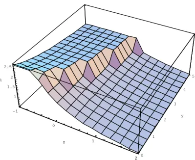
In order to look at welfare issues, we analyze the consequences of the introduction of layo¤ taxes on the consumption index c+ z` of all type-(y; z) of individuals. Inactive individuals, with z > Z(y); get a consumption index equal to z + ½ and active individuals, with z · Z(y); get w(y) = Z(y) + ½: Figure 1 displays the relative consumption gains (c+z`)c+z`¤¡(c+z`) resulting from the introduction of layo¤ taxes where (c + z`)¤denotes the value of the consumption index in the economy with layo¤ taxes and (c + z`) stands for the consumption index in the economy without layo¤ taxes. It can be seen that all individuals are strictly better-o¤ in the economy
15We compare steady states. Details are given in Appendix C.3.
-1 0 1 2 z 0 1 2 3 4 5 y 1 1.5 2 2.5 % -1 0 1 2 z
Figure 1: Consumption gains (in %) resulting from the introduction of layo¤ taxes in the Rawlsian economy.
with layo¤ taxes than in the economy without layo¤ taxes. The maximal increase (measured in percentages) in the consumption index is equal to 2.65 percent. The relative increase in the consumption index is larger for the individuals with low productivity. It is also larger for the individuals who participate in the labor market (because their wage increases more than the garantee income) than for those who are inactive.
5.2 Robustness checks
The quantitative impact of layo¤ taxes on aggregate output, employment and welfare is closely related to the job destruction and creation process. From this point of view, the arrival rate of job o¤ers, ¸; and the arrival rate of productivity shocks, ¹; turn out to have a strong in‡uence on the quantitative impact of layo¤ taxes. This issue is illustrated in Tables 2 and 3 where di¤erent values of the arrival rates of job o¤ers and productivity shocks are considered. All the other parameters remain unchanged.
¸ Emp rate ¢ Output (%) ¢ Emp (%) ¢ Income guarantee (%)
1 (benchmark) 60.00 1.93 3.45 1.64
2 63.88 0.52 0.94 0.45
3 65.27 0.23 0.44 0.21
Table 2: Robustness checks: changes in output, employment rate and guarantee income induced by the introduction of layo¤ taxes for di¤erent values of the arrival rate of job o¤ers.
when optimal layo¤ taxes are introduced for di¤erent values of the arrival rate of job o¤ers. As we have considered a low value of the arrival rate of job o¤ers in the benchmark economy, corresponding to a typical Continental European country with long unemployment spells, we look at higher values of ¸: As all the other parameters remain unchanged, the higher value of the arrival rate of job o¤ers changes the employment rate, whose value is given in the …rst column of Table 2. Table 2 shows that the gains induced by the introduction of layo¤ taxes decrease with the arrival rate of job o¤ers. It is because the social cost of job destruction (de…ned in equation (13)) increases with the length of the unemployment spell. Accordingly, the introduction of layo¤ taxes yields higher returns in economies where the duration of unemployment is longer.
Table 3 shows what happens with di¤erent values of the arrival rate of productivity shocks. Let us recall that the job destruction rate amounts to 11.11 percent in the benchmark, which is a relatively low value. Therefore, we look at higher values of the arrival rate of productivity shocks. These higher values lead to lower employment rates whose values are given in the …rst column of Table 3.
It appears that the gains induced by the introduction of layo¤ taxes get larger when the ar-rival rate of productivity shocks is raised. As unemployment increases with this parameter, these results also suggest that layo¤ taxes become more e¢cient in economies where unemployment is high.
¹ Emp rate ¢ Output (%) ¢ Emp (%) ¢ Income guarantee (%)
0.117 (benchmark) 60.00 1.93 3.45 1.64
0.15 58.02 2.84 5.11 2.40
0.20 55.32 4.48 8.17 3.75
Table 3: Robustness checks: change in output employment rates and income guarantee induced by the introduction of layo¤ taxes for di¤erent values of the arrival rate of productivity shocks.
6 Conclusion
This paper shows that optimal tax-subsidy schemes should comprise layo¤ taxes. It turns out that optimal layo¤ taxes are linked to the intensity of the redistribution of income: the optimal layo¤ tax is equal to the social cost of job destruction, which amounts to the discounted value of the unemployment bene…ts paid to the …red worker plus the payroll taxes (used to redistribute income across individuals with di¤erent abilities or di¤erent tastes for leisure) that the state losses when the job is destroyed. Accordingly, layo¤ taxes should represent a larger share of the wage when there are higher payroll taxes due to a more intensive redistribution of income.
Moreover, quantitative exercises suggest that the absence of layo¤ taxes found in most ac-tual tax-subsidy schemes can give rise to signi…cant welfare losses. Our benchmark simulation indicates that the introduction of layo¤ taxes may increase the employment rate by 3.5 percent and increase GDP by 2 percent in economies in which the redistribution of income is close to the La¤er bound.
Although we think that our result according to which optimal tax-subsidy schemes should comprise layo¤ taxes is general and relevant, our analysis needs to be further developed in some directions. First, our framework takes into account only some externalities induced by job de-struction decisions. Actually, search and matching models stress that job dede-structions induce search externalities which imply that the decentralized equilibrium does not yield enough job destructions (Aghion and Howitt, 1998, Mortensen and Pissarides, 1999). From this perspective, it would be worth introducing negative layo¤ taxes (Cahuc and Zylberberg, 2004, chapter 10).
We need to know more on the interactions between externalities and on their relative magnitude to know the optimal level of layo¤ taxes. Second, our framework assumes a very simple form of labor contracts, without ex-post bargaining that gives rise to hold-up problems. Moral hazard linked to unemployment insurance has also been neglected. Such issues, which have been ex-plored by Blanchard and Tirole (2004) in a static framework without heterogenous individuals, are worth studying. Third, our assumption of an exogenous arrival rate of job o¤ers does not allow us to account for the reaction of job creation to changes in the tax-subsidy schemes. These developments are on our research agenda.
References
Abowd, J.and Kramarz, F. (2003), “The Costs of Hiring and Separations”, Labour Economics, 10(5), pp. 499-530.
Aghion, P. and Howitt, P. (1998), Endogenous Growth Theory, Cambridge, Mass: Harvard University Press.
Anderson P. and Meyer B. (1993), “Unemployment Insurance in the United States: Layo¤ Incentives and Cross Subsidies”, Journal of Labor Economics, 11(2), pp. 70-95.
Anderson P. and Meyer B. (2000), “The E¤ects of the Unemployment Insurance Payroll Tax on Wages, Employment, Claims and Denials”, Journal of Public Economics, 78, pp. 81-106.
Azariadis, C. (1975), “Implicit contract and underemployment equilibria”, Journal of Political Economy, 83(6), pp. 1183-1202.
Baily, M. (1974), “Wages and employment under uncertain demand”, Review of Economic Studies, 41(1), pp. 37-50.
Beaudry, P. and Blackorby, C. (1997), “Taxes and Employment Subsidies in Optimal Redistri-bution Programs,” Discussion Paper 22, University of British Columbia.
Blanchard, O. and Tirole, J. (2004), “The Optimal Design of Labor Market Institutions. A First Pass”, NBER working paper 10443.
Burdett, K. and Wright, R. (1989a), “Unemployment Insurance and Short-Time Compensation: The E¤ects on Layo¤s, Hours per Worker and Wages”, Journal of Political Economy, 97, pp. 1479-1496.
Burdett, K. and Wright, R. (1989b), “Optimal Firm Size, Taxes, and Unemployment”, Journal of Public Economics, 39, pp. 275-287.
Cahuc, P. and Malherbet, F. (2004), “Unemployment Compensation Finance and Labor Market Rigidity”, Journal of Public Economics, 88, pp. 481-501.
Cahuc, P. and Zylberberg, A. (2004), Labor Economics, Cambridge, Mass: MIT Press.
Choné, P. and Laroque, G. (2005): “Optimal Incentives for Labor Force Participation,” Journal of Public Economics, 89, pp. 395-425.
Chui, H. and Karni, E. (1998), “Endogenous Adverse Selection and Unemployment Insurance”, Journal of Political Economy, 106, pp. 806-827.
Diamond, P. (1980), “Income Taxation with Fixed Hours of Work,” Journal of Public Economics, 13, pp. 101-110.
Feldstein M. (1976), “Temporary Layo¤s in the Theory of Unemployment”, Journal of Political Economy, 84, pp. 937-957.
Hopenhayn, H. and Nicolini, J., (1997), “Optimal Unemployment Insurance”, Journal of Polit-ical Economy, 105, pp. 412-438.
Laroque, G. (2005), “Income Maintenance and Labor Force Participation”, Econometrica, 73, pp. 341-73.
Ljungqvist, L. and Sargent, T. (2000), Recursive Macroeconomic Theory, Cambridge, Mass: MIT Press.
Mirrlees, J. (1971), “An Exploration in the Theory of Optimum Income Taxation,” Review of Economic Studies, 38, pp. 175-208.
Pissarides, C. (2001), “Employment Protection”, Labour Economics, vol 8, 131-159.
Mortensen, D. and Pissarides, C. (1999), “New Developments in Models of Search in the Labor Market”, in Ashenfelter, O. and Card, D. (eds), Handbook of Labor Economics, Elsevier Science Publisher, vol 3B, chapter 39.
Rosen, S. (1985), “Implicit Contracts: A Survey”, Journal of Economic Literature, vol 23, pp. 1144-1175.
Saez, E. (2002), “Optimal Income Transfer Programs: Intensive versus Extensive Labor Supply Responses,” Quarterly Journal of Economics, 117, pp. 1039-1073.
Appendix
A Proof of Proposition 1
Necessary conditions have been shown in the text. It remains to be proved that any feasible allocation which satis…es conditions 1, 2 and 3 is Pareto optimal. Let us show that an allocation that makes every agent as least as well o¤ and some strictly better o¤ than an allocation which satis…es conditions 1, 2 and 3 is not feasible.
The feasibility constraint for a …rst-best allocation which satis…es conditions 1, 2 and 3 and yields consumptions denoted by c(y; z) reads
Z
SA
Y¤(y)h(y; z)dydz = Z
SA
c(y; z)h(y; z)dydz + Z
SI
c(y; z)h(y; z)dydz; where Y¤(y) = yR+1
0 xdG(x)¡ k(y) stands for the average …rst-best net production of employees with
ability y.
Let us denote by ^c(y;z; x) the consumption of type-(y; z) active individuals and by ^c(y; z) the con-sumption of type-(y; z) inactive individuals for a feasible allocation (called henceforth the alternative allocation) that makes every individual at least as well o¤ and some strictly better o¤ than a …rst-best allo cation (called henceforth the initial allocation) which satis…es conditions 1, 2 and 3 and yields consumptions denoted by c(y; z).
The feasibility constraint for the alternative allocation reads Z SA^ ^ Y (y)h(y; z)dydz = Z SA^ µZ R ^ c(y; z; x)dG(x) ¶ h(y; z)dydz + Z SI^ ^
c(y; z)h(y; z)dydz;
where ^Y (y) = yRW (y)^ xdG(x)¡ k(y) stands for the average net production of employees with ability y
and SA^, SI^denote the set of active and inactive individuals respectively.
Let us denote by SA ^A the set of agents who are active in both allocations, by SI ^I the set of those who are inactive in both allocations, by SA ^I the set of those who are active for the initial allocation and inactive for the alternative allocation, by SI ^A the set of those who are inactive for the initial allocation and active for the alternative allocation. By de…nition one gets:
Z SA ^A µZ R^c(y; z; x)dG(x) ¶ h(y; z)dydz + Z SI ^I ^
c(y; z)h(y; z)dydz¸ Z
SA ^A[SI ^I
c(y; z)h(y; z)dydz Z
SA ^I
[^c(y; z) + z] h(y; z)dydz¸ Z
SA ^I
c(y; z)h(y; z)dydz Z SI ^A µZ R^c(y; z; x)dG(x) ¶ h(y; z)dydz¸ Z SI ^A
with some strict inequality. Summing up the three previous equations yields Z SA^ µZ R^c(y; z; x)dG(x) ¶ h(y; z)dydz + Z SI^ ^
c(y; z)h(y; z)dydz > Z
S
c(y; z)h(y; z)dydz + Z
SI ^A
zh(y; z)dydz¡ Z
SA ^I
zh(y; z)dydy: (A1)
From condition 3 it follows that Z SI ^A zh(y; z)dydz¸ Z SI ^A Y¤(y)h(y; z)dydz Z SA ^I zh(y; z)dydz· Z SA ^I Y¤(y)h(y; z)dydz:
These two equations imply, together with (A1): Z SA^ µZ R ^ c(y; z; x)dG(x) ¶ h(y; z)dydz + Z SI^ ^
c(y; z)h(y; z)dydz > Z
S
c(y; z)h(y; z)dydz + Z SI ^A Y¤(y)h(y; z)dydz¡ Z SA ^I Y¤(y)h(y; z)dydz:
As c(y; z) is feasible, it satis…es Z
S
c(y; z)h(y; z)dydz = Z SA ^I[SA ^A Y¤(y)h(y; z)dydz; which yields Z SA^ µZ Rc(y; z; x)dG(x)^ ¶ h(y; z)dydz + Z SI^ ^
c(y; z)h(y; z)dydz > Z SA ^I[SA ^A Y¤(y)h(y; z)dydz + Z SI ^A Y¤(y)h(y; z)dydz¡ Z SA^I Y¤(y)h(y; z)dydz = Z SI ^A[SA ^A Y¤(y)h(y; z)dydz: As SA^= SA ^A[ SA ^I;one gets: Z SA^ µZ R^c(y; z; x)dG(x) ¶ h(y; z)dydz + Z SI^ ^
c(y; z)h(y; z)dydz > Z
SA^
Y¤(y)h(y; z)dydz:
From the productive e¢ciency condition 1 one has Y¤(y) ¸ Y (y); 8y. This condition implies, together
with the previous inequality: Z SA^ µZ R^c(y; z; x)dG(x) ¶ h(y; z)dydz + Z SI^ ^
c(y; z)h(y; z)dydz > Z
SA^
Y (y)h(y; z)dydz; which proves that the alternative allocation is not feasible. ¥
B Proof of Proposition 3
Let us …rst notice that when the state implements the tax-subsidy scheme fb(w); ¿(w); f(w); ½g, the equilibrium wage is an increasing function of y that is denoted by w(y). The equilibrium values of the other variables can be denoted as b(y) = b(w(y)); ¿(y) = ¿ (w(y), f (y) = f (w(y)); X(y) = X(w(y); y); q(y) = G (X(y)) and Z(y) = Z(w(y); y):
Proposition 3 is proved as follows. First, we de…ne the optimal value of fw(y); b(y); X(y); ½g for any second-best …nancial incentives to work ~Z(y) · Y¤(y). Then we …nd out how this solution can be
implemented by the appropriate choice of f¿(w); b(w); f(w); ½g : The budget constraint of the state reads
Z +1 ymin
ÃZ Z( y)
¡1 f[1 ¡ G(X(y))] ¿(y) + G(X(y)) [f (y) ¡ b(y)]g h(y; z)dz
! dy¸ ½ · 1¡ Z +1 ymin H [y; Z(y)] dy ¸ ; (B1) where H [y; Z(y)] =R¡1Z (y)h(y; z)dz. Using the free entry condition:
Z +1 X (y)
[x¢ y ¡ w(y) ¡ ¿ (y)] dG(x) ¡ G(X(y))f (y) = k(y); 8y ¸ ymin; (B2)
the budget constraint of the state (B1) can be rewritten as: Z +1
ymin
fY (y) ¡ [1 ¡ G(X(y))] w(y) ¡ G(X(y))b(y)g H [y;Z(y)] dy ¸ ½ · 1¡ Z +1 ymin H [y; Z(y)] dy ¸ (B3) where Y (y) = yR+1 X (y)xdG(x)¡ k(y):
Accordingly, the maximization problem which de…nes the optimal value of fw(y); b(y); X(y); ½g for any second-best …nancial incentives to work ~Z(y)· Y¤(y) reads
max
fw(y);b(y);X(y);½g½
sub ject to
vhZ(y) + ½~ i= [1¡ G(X(y))]v (w(y)) + G(X(y))v(b(y)); 8y ¸ ymin (B4)
Z +1 ymin
fY (y) ¡ [1 ¡ G(X(y))] w(y) ¡ G(X(y))b(y)gHhy; ~Z(y)idy¸ ½ · 1¡ Z +1 ymin Hhy; ~Z(y)idy ¸ : (B5) Let us denote by ¸(y) and ¹ the Lagrange multipliers associated with constraints (B4) and (B5) respectively. The Lagrangian reads
L=½ + Z +1
ymin
¸(y)n[1¡ G(X(y))] v (w(y)) + G(X(y))v(b(y)) ¡ vhZ(y) + ½~ iody+ ¹
·Z +1
ymin
fY (y) ¡ [1 ¡ G(X(y))] w(y) ¡ G(X(y))b(y)g Hhy; ~Z(y)idy¡ ½ · 1¡ Z +1 ymin Hhy; ~Z(y)idy ¸¸
The …rst-order conditions can be written as @L
@X(y) = 0, ¸(y) [v
0(b(y))¡ v0(w(y))] = ¹ (yX(y)¡ [w(y) ¡ b(y)]) Hhy; ~Z(y)i; 8y ¸ y
min; (B6)
@L
@w(y) = 0, ¸(y)v0(w(y)) = ¹H h y; ~Z(y)i; 8y ¸ ymin; (B7) @L @b(y) = 0, ¸(y)v 0(b(y)) = ¹Hhy; ~Z(y)i; 8y ¸ y min; (B8) @L @½ = 0, 1 ¡ Z +1 ymin ¸(y)v0hZ(y) + ½~ idy = ¹ · 1¡ Z +1 ymin Hhy; ~Z(y)idy ¸ : (B9)
Equations (B7) and (B8) imply that b(y) = w(y) = ~Z(y) + ½;8y ¸ ymin. As w(y) = ~Z(y) + ½; equation
(B7) reads ¸(y)v0( ~Z(y) + ½) = ¹Hhy; ~Z(y)i which yields in (B9): ¹ = 1: Thus, equation (B7) implies
that ¸(y) > 0; 8y ¸ ymin:Eventually, when b(y) = w(y); ¸(y) > 0; 8y ¸ ymin and ¹ > 0, equation (B6)
implies that X(y) = 0:
At this stage, it has been proved that the optimal value of fw(y); b(y); X(y); ½g satis…es b(y) = w(y) and X(y) = 0 for any second-best …nancial incentives to work ~Z(y)· Y¤(y): Theses properties transform
our model into a particular version of Laroque’s (2005) model of labor supply decisions at the extensive margin with no unemployment. Our model is now such that a type-(y; z) agent who decides to “work” produces Y¤(y) and earns an income equal to ~Z(y) + ½; if he decides to stay idle he produces nothing
and earns z + ½: Theorem 3 in Laroque (2005) completely characterizes the second-best optimal …nancial incentives to work ~Z(y) in this case. It is shown that feasible …nancial incentives to work ~Z(y); such that
~
Z(y) · Y¤(y); support a second-best allocation if and only if no category of ability y is overtaxed at
~ Z(y):
The optimal value of ½ can be obtained by substituting the values of w(y) and b(y) which are equal to ~Z(y) + ½ into the – binding – constraint (B5). One gets ½ =Ry+1
min
h
Y¤(y)¡ ~Z(y)iHhy; ~Z(y)idy:Let
us …nd out how this solution can be implemented by the appropriate choice of f¿(w);b(w); f(w); ½g : The equality b(y) = w(y) is merely implemented by b(w) = w which proves condition 1. of Proposition 3.
The appropriate choice of ¿(w) and f (w) can be de…ned by noticing that there exists a bijection between (¿(y); f (y)) and (w(y); X(y)) which is de…ned by two equations: namely the reservation produc-tivity of the …rms (equation (4))
X(y) = w(y) + ¿ (y)¡ f (y)
y ; 8y ¸ ymin; (B10)
and the free entry condition (B2), which reads, using the de…nition of the reservation productivity of the …rms (B10):
f (y) =¡k(y) + Z +1
X(y)