Three-dimensional analysis of a tensile test on a propellant with digital volume correlation

HAL Id: hal-00634714

https://hal.archives-ouvertes.fr/hal-00634714

Submitted on 22 Oct 2011

HAL is a multi-disciplinary open access

archive for the deposit and dissemination of

sci-entific research documents, whether they are

pub-lished or not. The documents may come from

L’archive ouverte pluridisciplinaire HAL, est

destinée au dépôt et à la diffusion de documents

scientifiques de niveau recherche, publiés ou non,

émanant des établissements d’enseignement et de

Three-dimensional analysis of a tensile test on a

propellant with digital volume correlation

François Hild, Alain Fanget, Jérôme Adrien, Eric Maire, Stéphane Roux

To cite this version:

François Hild, Alain Fanget, Jérôme Adrien, Eric Maire, Stéphane Roux. Three-dimensional analysis

of a tensile test on a propellant with digital volume correlation. Archives of Mechanics, 2011, 63 (5-6),

pp.1-20. �hal-00634714�

Three dimensional analysis of a tensile test on a

propellant with digital volume correlation

Fran¸cois Hild,

_{Alain Fanget,}

_J´

_erˆ

_{ome Adrien,}

Eric Maire

_{and St´}

_{ephane Roux}

a

_{Laboratoire de M´}

_{ecanique et Technologie (LMT-Cachan)}

ENS Cachan / CNRS / UPMC / PRES UniverSud Paris

61 Avenue du Pr´

esident Wilson, F-94235 Cachan Cedex, France

Email:

{francois.hild,stephane.roux}@lmt.ens-cachan.fr

b

_{Centre d’Etudes de Gramat (CEG)}

BP 80200, F-46500 Gramat, France

Email: alain.fanget@cea.fr

c

_{Laboratoire Mat´}

_{eriaux, Ing´}

_{enierie et Sciences (MATEIS)}

INSA-Lyon / UMR CNRS 5510

7 avenue Jean Capelle, F-69621 Villeurbanne, France

Email:

{jerome.adrien,eric.maire@insa-lyon.fr}

∗

_{corresponding author}

Abstract:

A full three dimensional study of a tensile test on a sample made of polymer-bonded propellant is presented. The analysis combines different tools, namely, X-ray microtomography of an in situ experiment, image acquisition and treat-ment, 3D volume correlation to measure three dimensional displacement fields. It allows for global and local strain analyses prior to and after the peak load. By studying the correlation residuals, it is also possible to analyze the damage activity during the experiment.

Keywords:

Correlation residuals, damage mechanism, measurement uncertainty, strain het-erogeneities, volume correlation, X-ray microtomography.

1

Introduction

Propellant-like materials are a class of particulate composites with a very high volume fraction since the inclusions contain the active molecules. The associ-ated chemical energy is released either very quickly in explosives, or more slowly in rocket propulsion. In all cases, a large amount of hot gases is produced, and constitutes a serious hazard if they are not delivered when adequately stim-ulated, but rather when triggered by accidental or malevolent loading. The thermomechanical modeling of such class of materials in therefore needed to assess their vulnerability [1].

Homogenization procedures are carried out in order to describe the behavior of a propellant medium via a morphological approach in a finite transformations (viscohyperelasticity without damage [2, 3]) and in small perturbations when dealing with damage [4, 5]. These models are based on a schematization of the meso-structure extracted from a morphological analysis of microtomographic data. The constitutive laws of the constituents have been built only based upon

macroscopic data. However, on the one hand the loading conditions undergone by the matrix are very different from the macroscopic loading due to the strong contrast between the constituents; on the other hand no local data are avail-able on the debonding between the grains and the matrix, on the initiation and propagation of cracks in the medium. The validation of these theoretical de-scriptions requires a confrontation of numerical simulations at the mesoscopic scale with experimental data at the same scale. This can be achieved thanks to the measurements of the local kinematic fields.

X-Ray Computed MicroTomography (XCMT) is a very powerful tool to have access to the details of the full microstructure of a material in a non destruc-tive fashion. By reconstruction from 2D radiographic projections, it allows for a 3D visualization of the different phases of a material [6, 7]. By analyzing these 3D reconstructed volumes, one has access, for instance, to damage mech-anisms in the bulk of particulate composites [8, 9, 10]. Cellular materials have also been studied [11, 12], and 2D [13] or 3D [14, 15] displacement and strain measurements were performed.

The analysis of mechanical tests on explosives was already carried out by using 2D Digital Image Correlation (DIC). The natural texture of the material was analyzed [16] or a random pattern was sprayed [17] to determine in-plane displacements in the analysis of crack inception and crack propagation [18, 19]. DIC was also used to estimate the size of the representative volume element [20] for this type of granular materials. Localized shear bands under quasi static [17] and dynamic [21] loadings could be visualized and quantified. Last, the creep properties of such materials [22] were studied thanks to full field measurements. To the authors’ knowledge, 3D analyses were never performed before on this type of material.

In the following, a Galerkin approach to digital volume correlation [14] is used to measure displacement and evaluate strain fields during a tensile test on a propellant. In Section 2, the studied material, the experimental configuration and the imaging system are presented. The correlation algorithm used herein

is briefly recalled in Section 3 and its a priori performance is evaluated by artificially moving a reference volume. This type of analysis enables for the evaluation of measurement uncertainties in terms of displacements and strains. The experimental results are finally analyzed globally in Section 4 and locally in Section 5 where strain fields and correlation residuals are considered. The global strain analysis allows us to extract a macroscopic Poisson’s ratio, and the local analyses yield mean strains and their fluctuations in each phase that might be compared to the predictions of homogenization results. Last, the correlation residuals are used to assess the damage mechanism and state of the studied material.

2

Experimental configuration

Figure 1 shows the sample before the test and a microtomographic slice of the studied material. The latter is a dummy propellant made of ammonium hexafluorite grains in a polymeric matrix (HTPB). It is a concrete-like mate-rial containing a unimodal distribution of grains (i.e., the aggregates) centered around 400 µm in diameter embedded in a polymeric matrix (i.e., the mortar). The grains represent 75.4 wt.% of the composite (or≈ 59 vol.%). The diameter of the gauge section is equal to 10 mm and the total length is equal to 50 mm. Synchrotron X-Ray microtomography is a computed method allowing the user to measure the 3D map of the attenuation coefficient of a sample. This map is retrieved from a set of radiographs taken under different viewing angles. More details about the method can be found in [6]. The tomograph used in the present study is located at beamline ID19 of the European Synchrotron Radiation facility (ESRF) in Grenoble (France). For the present experiment, this tomograph was operated as follows. The voxel size of the medium reso-lution detector was set to 7.4 µm and the detector dimensions were restricted by software to 1500 (horizontal) ×1024 (vertical) pixels. The beam was gen-erated by an undulator, the gap of which was closed at 12.5 mm. The beam

was then monochromated to 25 keV using a double crystal vertical monochro-mator. The distance between the detector and the sample was set to 80 mm. For each scan, a total of 1500 radiographs were recorded while the sample was rotated over 180◦. The exposure time for each radiograph was 0.2 s and the to-tal scan time (including exposure, transfer to disk and rotation) was just below 10 minutes. The reconstruction was performed using PyHST software available at ESRF [23]. It should be noted that three consecutive scans, with a vertical displacement of the sample between each scan, were needed to image the entire useful length of the sample. In what follows, the results are extracted from the scan in which the final failure plane was located.

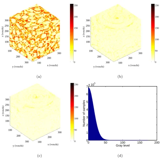
Image and/or volume correlations require a random texture to measure dis-placements. The hexafluorite grains are extremely helpful for the registration, as they constitute a random marking with a high contrast distributed within the specimen. As can be seen in Figure 2(a), they appear as light spheres with a well defined morphology. The dynamic range of the reconstructed volumes is equal to 8 bits. The mean gray level is 157 and the corresponding standard deviation is 56, which is a high value due to the bimodal distribution. As seen on the histogram of Figure 2(b), the whole dynamic range is used. A bimodal distribution allows for the separation of the matrix (i.e., gray levels less than 146) and the inclusions (i.e., gray level greater than 146). In this study, the size of the reconstructed volumes is 400× 400 × 400 voxels, and the analyzed region of interest (ROI) is centered and has a size of 272× 272 × 272 voxels (all the results presented herein are performed on a standard PC with an i7 core CPU @ 2.8 GHz and a 2-Go RAM). The computation time per couple of analyzed volumes lasted on average one hour when about 130,000 degrees of freedom (i.e., for 8-voxel elements) were measured.

A specially designed testing machine set on the rotation stage of the to-mograph allowed tension to be applied to the sample during the experiment. The interrupted in situ procedure was used in the present study i.e., the dis-placement of the mobile grip was stopped during the 10 minutes required for

the acquisition of the radiographs to prevent blurring of the images and the structural evolution of the sample during the scan. The tensile machined hav-ing a load cell and a displacement sensor, the tensile curve could be monitored during the mechanical test. A detailed description of this rig can be found in Ref. [24]. The displacement speed was set to 0.4 µm/s. Given the gauge length of the sample, this corresponded to≈ 10−5s−1mean strain rate. Six scans were acquired for the analyzed test. Apart from the reference scan, i.e., before any load was applied, three scans were taken up to the peak load and one thereafter (Figure 3). The last one was performed after failure (Figure 2(c)) and is not analyzed herein.

3

Digital Volume Correlation (DVC)

In this section, the correlation algorithm is first presented. Its performance is evaluated by using an a priori analysis whereby a reference volume is artificially moved and the displacement and strain uncertainties are evaluated.

3.1

Galerkin approach to DVC

Volume correlation consists in registering the texture of two volumes, namely a first one f in the reference configuration, and another one g in the deformed configuration. To estimate the unknown displacement field U(X), the quadratic difference φ2_{(X) = [f (X)− g(X + U(X))]}2 _{is integrated over the studied}

do-main Ω

Φ2= ∫

Ω

φ2(X) dX (1) and minimized with respect to the degrees of freedom ai of the measured

dis-placement field

U(X) =∑

i

aiNi(X) (2)

where Ni(X) are the components of the chosen kinematic basis. In the present

case, a 3D finite element kinematics is chosen [25] for the sought fields, so that Nicorrespond to the shape functions, here chosen as trilinear polynomials

associated with 8-node cube elements (or C8-DVC [14]). Other approaches can be found, namely, as in 2D applications, the most commonly used correlation algorithms consist in registering locally small zones of interest in a sequence of pictures to determine local displacement components [26]. The same type of hypotheses are made in three-dimensional algorithms [27, 28, 29, 30].

3.2

A priori analysis

Before studying the displacement field between two actual volumes, it is impor-tant to evaluate the level of uncertainty attached to both the natural texture of the image and the algorithm used. Integer valued displacements do not involve any approximation in the determination of the gray level value. Conversely, any sub-voxel estimate relies on gray level interpolation. Consequently, the resolu-tion of the technique is dependent on the way the gray levels are interpolated in addition to other effects associated with the reconstruction process of any tomography [31]. In the present case, a cubic interpolation is used. To as-sess the uncertainty resulting from this interpolation, a uniform displacement (Up, Up, Up) is prescribed to the reference volume (Figure 2(a)) to produce an

ar-tificial (i.e., “shifted”) volume when Up = 0.5 voxel. The correlation procedure

is then run blindly on this pair of volumes. The systematic error is measured from the spatial average of the determined displacement. The uncertainty is measured from the standard deviation of the displacement field σ(U ). The sys-tematic error was quite small as compared to the uncertainty. Only the latter is reported herein.

To assess the quality of a correlation result, the correlation residuals are the only data available when the measured displacements are not known. In the following, the normalized correlation residual is considered

η(X) = |φ(X)|

maxΩ(f )− minΩ(f )

(3)

and its mean value ⟨η⟩ is computed over the whole correlation volume Ω. To quantify the strain uncertainty, the mean principal strains ϵi are estimated over

the entire region of interest for each rigid body translation.

The assessment of the uncertainty for different element sizes is very impor-tant since it allows one to determine the optimal element size to be used for a given constraint on the error bars. Large elements will enable for accurate determinations of displacements because of the large number of voxels involved in each element. Conversely, they are unable to capture complex displacement fields with rapid spatial variations. Conversely, a small element will be flexible enough to measure large displacement gradients, but will give less accurate re-sults. In the present analysis, only one value is chosen, namely, Up= 0.5 voxel

since it leads to the maximum uncertainties [15].

The uncertainty (here defined as the maximum standard deviation for sub-voxel displacements) σ(U ) is observed, in three dimensions, to vary as a power-law function of the element size ℓ [14, 15]

σ(U )≈ Aα+1ℓ−α (4)

where A is a constant whose level is of the order of one voxel. The power α characterizes the decay of the displacement uncertainty with the element size. Figure 4 shows that a power-law dependence is obtained in three dimensions, where a best fit through the data produces the dashed line in the graph, with

A ≈ 1 voxel and α = 1. The mean correlation residual ⟨η⟩ is equal to 2.4 %

for all analyzed sizes. This result is consistent with the fact that the kinematic basis is able to capture the prescribed kinematics, irrespective of the element size.

In terms of strain levels, two quantities are analyzed, namely the mean strain level (to be defined in Section 4), and the standard deviation of average strains per element (see Section 5). It is worth remembering that both quantities should be equal to 0 if the registration were perfect. For the mean strain level, the maximum bias (i.e., 3× 10−4) is observed for 8-voxel elements. It reaches values less than 10−4 for elements whose size is greater than 32 voxels. The standard deviation of strains is equal to 6× 10−3 for 8 voxel elements and decreases down to about 10−4 for 48-voxel elements.

4

Macroscopic analysis of the tensile test

The element size is first equal to 16 voxels, which is a compromise (Figure 4) between the uncertainty level, the spatial resolution (i.e., the element size), and the computation time (i.e., of the order of 20 minutes per analysis). The reference volume is always the same and four loading steps could be analyzed with a good convergence of the algorithm.

4.1

Strain evaluations

From the analyzed displacement field, the mean strains are determined over the whole ROI. Even though the level of strains will remain moderate on average (i.e., less than 2 %), larger values may appear due to the coarse microstructure (Figure 2(a)). In the present case, the infinitesimal strain assumption is not made locally. Consequently, a large transformation framework is used. The deformation gradient tensor F is considered. The latter is related to the dis-placement U by

F = 1 +∇U (5)

where 1 denotes the second order unit tensor. A polar decomposition of F is used [32]

F = RS (6)

where R is an orthogonal tensor (R−1= Rt_{) describing the rotations, and S the}

right stretch tensor (S = St_{). From the latter, the nominal (or Cauchy-Biot)}

strain tensor ϵ = S− 1 will be used. When averaged over the whole region of interest Ω, the mean nominal strain tensor is defined as

⟨ϵ⟩ = ⟨S⟩ − 1 (7)

where⟨S⟩ is evaluated by considering the mean deformation gradient ⟨F⟩

⟨F⟩ = 1 +_|Ω|1

∫

∂Ω

U⊗ N dS (8)

and N denotes the outward normal vector to the external boundary ∂Ω of the ROI Ω. The principal strains are subsequently determined, and the apparent

Poisson’s ratio ν is defined as

ν =−⟨ϵ2⟩ + ⟨ϵ3⟩

2⟨ϵ1⟩

(9)

where⟨ϵ1⟩ is the maximum principal strain (i.e., ⟨ϵ1⟩ > |⟨ϵ2⟩|, |⟨ϵ3⟩|). The above

definition of an appparent Poisson’s ratio coincide with the standard expression at small strains. At larger strains, this is only to be interpreted as a convenient dimensionless quantity that captures the relative change of volume as compared to the deviatoric part. A more exhaustive analysis would require the formulation and identification of a damage constitutive law on a large scale, which is beyond the scope of the present analysis. Moreover, as damage quickly concentrates on the to-be failure surface, this signals the onset of a localization behavior that is not amenable to a continuum description, nor to a classical identification procedure.

4.2

Analysis of the four loading steps

Figure 5 shows three residual maps when the first load level is analyzed. The first map corresponds to the initial volume difference when no corrections are made (Figure 5(a)). There is a clear mismatch between the two analyzed states. The corresponding value of⟨η⟩ is equal to 22.1 %. When an initial correction es-timated as a rigid body translation is performed, it leads to the second map that shows the effect of this first correction (Figure 5(b)). However, there are still zones in which the residuals are too high. The value of ⟨η⟩ decreases to 6.7 %. Last, the third map shows the residuals at convergence (Figure 5(c)). Except for a few points impacted by ring artifacts, the residuals are low everywhere. The mean correlation residual ⟨η⟩ is equal to 5.1 %. This result is confirmed when the shape and range of the histogram of correlation residuals |φ| (Fig-ure 5(d)) is compared with that of the initial text(Fig-ure (Fig(Fig-ure 2(b)). The former is monomodal and is essentially concerned with small gray levels as opposed to the latter that ranges from 0 to 255 gray levels with a bimodal distribution. This additional test is important, since it is only after having checked that the

residual field is small in the whole ROI that the results are deemed trustworthy. This first analysis deals with moderate strain levels (⟨ϵ1⟩ ≈ 0.29 %), and the

mean transverse strain (⟨ϵ2⟩ + ⟨ϵ3⟩)/2 is equal to −0.145 %. These values allow

for the determination of the macroscopic Poisson’s ratio here equal to 0.5. This value corresponding to an incompressible material is to be expected since the binder is made of an incompressible material. The role of the HMX grains is not significant in the early stages of deformation.

The major strain levels ⟨ϵ1⟩ increase (i.e., 0.78, 1.10, 1.68 %, respectively)

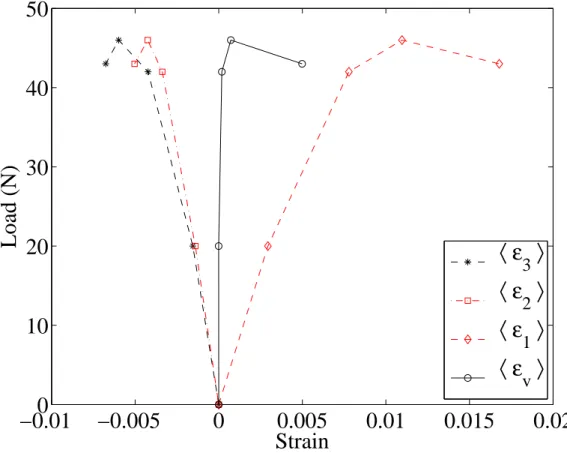
for the three subsequent load steps. The corresponding Poisson’s ratios are 0.49, 0.47, 0.35. Up to the peak load, the value of the latter is virtually iden-tical and equal to that of an incompressible material. Beyond the peak load, it decreases, signalling displacement heterogeneities, which will be analyzed in the sequel. This result is also confirmed when the mean strains are plotted as functions of the applied load (Figure 6). In particular, the volumetric strain

⟨ϵv⟩ = ⟨ϵ1⟩ + ⟨ϵ2⟩ + ⟨ϵ3⟩ remains vanishingly small except for the last analyzed

level, where it becomes significantly positive (i.e., dilatancy is observed). Fur-thermore, as the mean strain level increases, the transverse behavior becomes less isotropic (i.e.,⟨ϵ2⟩ ̸= ⟨ϵ3⟩). This effect is due to an anisotropic degradation,

as will be shown below. The mean correlation residuals⟨η⟩ are equal to 5.5 %, 5.6 %, 5.9 %, signaling that the registration is mildly degrading when compared with the first load level (i.e., 5.1 %).

5

Local analyses of the whole sequence

5.1

Strain fields

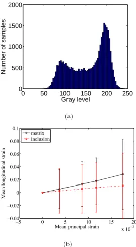
In the following analyses, the element size ℓ is decreased to 8 voxels to corre-late the strain fields to the underlying microstructure. Figure 7(a) shows the histogram of mean gray level in each considered element. The latter’s shape (at the element scale) is reminiscent of that observed at the voxel scale (see Figure 2(a)). This is not the case for elements whose size is greater than 8

voxels. From the measured displacement field, average strains per element are evaluated by following the same approach as in the previous section. The mean nominal strain tensor is defined as

ˆ

ϵ = ˆS− 1 (10)

where ˆS is evaluated by considering the mean deformation gradient ˆF over an element Ωe ˆ F = 1 + 1 |Ωe| ∫ ∂Ωe U⊗ N dS (11)

and N denotes the outward normal vector to the external boundary ∂Ωe.

In the following, the elements containing parts of an inclusion are defined such that their mean gray level is greater than 146. Conversely, elements whose gray level is less than 146 are considered as belonging to the matrix. Figure 7(b) shows the mean value and standard deviation (error bars) of the normal strains in the matrix and in the inclusion as a function⟨ϵ1⟩. The fluctuations are very

important, and well above the strain uncertainties assessed in Section 3. They are deemed trustworthy. They are due to the high volume fraction of inclusions (i.e., 62 % with the definition used herein, to be compared with 62 % at the voxel level with the same convention) and their heterogeneous distribution in the composite. These values are close to the mean volume fraction given by the maker (i.e., 59 %). The hypotheses of Eshelby’s analysis [33] are clearly not valid in the present case of a high volume fraction of inclusions. Furthermore, the mean longitudinal strains in the matrix are up to 2.7 times greater than those in the inclusions. This is due to the contrast of elastic properties of both materials. For the three first strain levels, the ratio is close to 2.3. The fact that the ratio increases is due to the development of damage in the sample. This is also observed when the fluctuations are analyze (i.e., error bars in Figure 7(b)).

5.2

Correlation residuals

The correlation residuals are commonly used to make sure that the registration was successful [14, 15, 34]. They enabled us to deem the previous results

glob-ally trustworthy. Various causes can lead to higher correlation residuals. First, the whole registration was not satisfactory. Second, the brightness conserva-tion is not satisfied. Third, the kinematic hypotheses are no longer fulfilled. For instance, when analyzing cracks, a C8 kinematic basis does not allow for displacement discontinuities. One solution is then to enrich the kinematic ba-sis [35] as in extended finite element method [36, 37]. The correlation residuals are then used to determine the 0-contour level set associated with crack sur-face [38]. This procedure will not be used herein. The analysis will be restricted to the correlation residuals and their change with the applied load when C8-DVC is utilized.

In the present case, a very coarse discretization is used (i.e., with 68-voxel elements) so that any deviation from a continuous field is detected. Figures 8 and 9 show cuts of correlation residuals in the vicinity of the crack plane. For the first load level, the registration was successful except in areas where ring artifacts appear. The mean correlation residual ⟨η⟩ is equal to 5.5 %. This value is higher when compared to the level observed when a 16-pixel discretiza-tion was used (i.e., 5.1 %). The fact that a coarser discretizadiscretiza-tion increases the correlation residual can be understood as local displacement fluctuations can-not be captured. The same conclusion can be drawn for the second load level. The value of the mean correlation residual ⟨η⟩ increases up to 6.1 %. For the third load level, high gray levels appear in zones initially free from reconstruc-tion artifacts. On a global scale, the mean correlareconstruc-tion residual⟨η⟩ is equal to 6.3 %. Last, for the fourth load level, the high correlation residuals are essen-tially located close to inclusion / matrix interfaces. Consequently, the main damage mechanism is related to interface debonding. This is also confirmed in Figure 2(b) where the final fracture path is essentially the result of multiple debonding. The mean value still increases to reach 6.9 %.

For Figures 8 and 9, as the mean strain level increases, more and more areas appear with high correlation residuals. The latter ones indicate that the gray level conservation is no longer satisfied. Of the two causes that can explain this

effect, namely, matrix / inclusion debonding and inclusion breakage, the former is dominant. The poor kinematics chosen in this part of the study allows for a better visualization of the zones where damage takes place. When compared with the cut of the deformed volume for which the mean rigid body translation was corrected, the correlation residuals indicate more areas where debonding oc-curred than by visual inspection of the reconstructed volumes themselves. This is presumably due to the resolution of the DVC technique, which is sub-voxel (Figure 4), and therefore it can reveal small displacement levels that cannot be detected by bare eyes.

Figure 10 shows a three dimensional visualization of the regions where the residuals have a high value. This sort of representation is helpful to analyze the spatial distribution of damage measured by correlation. At the beginning, the high values of the residuals are mainly associated with ring artifacts recogniz-able because they are axisymmetric (about the rotation axis). It is very clear however, at least for the fourth step, that high values of the residuals develop in polar regions of the inclusions, i.e., where the normal to these interfaces points toward the tensile axis, indicating matrix / inclusion debonding or fracture of one of the two constituents close to this interface. It should also be noted, that although less obvious, an increase of the residuals is detected for earlier steps in the same locations as the fourth step. Moreover, a larger density of debonding takes place within a region where the final fracture plane will develop. There-fore, failure can be interpreted as the coalescence of microcracks originating as polar debonding at particle / matrix interfaces. Last, microcracks also tend to propagate along larger area of the interface where they were initiated.

6

Summary

The analysis presented herein aims for a better understanding of the deforma-tion and damage mechanisms of propellants in which the volume fracdeforma-tion of inclusions is high (i.e., of the order of 60 %). It was shown that strain

hetero-geneities are very high even at moderate strain levels. Furthermore, debonding of the matrix / inclusion interfaces occurs at levels prior to the peak load and beyond. This type of information is very useful when modeling the behavior of such complex materials [2, 3, 4, 5].

All these results were obtained by resorting to Digital volume correlation. The latter is a powerful tool to analyze in situ experiments in a tomograph (here the beamline was that of a third generation synchrotron). It yields 3D displacement fields in the bulk of the studied material. The uncertainty levels are sufficiently low to perform analyses of strain fields even in the elastic regime of the studied material. Furthermore, the correlation residuals, which are usually used to assess the quality of the registration, were also used to analyze the damage mechanism seen as cause for non conservation of the gray levels since the kinematic basis was not consistent with the true one.

The results presented herein correspond to a first step that showed the fea-sibility of DVC to analyze the mechanical behavior of propellants. In terms of measurement procedures, two different paths may be followed to enrich the measured quantities. First, unstructured meshes may be used as was proposed in 2D analyses [39]. In the present case, the mesh topology should then be chosen in such a way that the interfaces between elements coincide with those between inclusions and the matrix. One should remain cautious since small elements would then lead to higher measurement uncertainties as shown herein (Figure 4). A mechanical regularization may then allow to lower the uncer-tainty [39]. Second, a voxel-scale discretization may also be considered. This approach requires always a mechanical regularization [40]. The main advantage though is that the discretization becomes the simplest one may consider and the gray level may then be used, as shown herein, to regularize the volume registration. Both approaches will be assessed in the future.

Another perspective is related to the use of the data obtained herein when compared to the predictions of developed models. This comparison can be performed on the macroscopic level by using the experimental boundary

condi-tions provided by the DVC measurements. It can also be performed on a local level thanks to the assessment of the strain distributions in the inclusions and the matrix. Last, the analysis of the damage mechanism and its quantifica-tion provides some very useful input on the modeling side for qualitative and quantitative estimates.

Acknowledgments

This work was supported by a DGA grant (no. 2009-008573). The experiments reported herein were performed with the help of Mrs. Boller at ESRF (ID19 beamline).

References

[1] H. Trumel, A. Dragon, A. Fanget and P. Lambert, A constitutive model for the dynamic and high-pressure behaviour of a propellant-like material: Part I: Experimental background and general structure of the model, Int.

J. Num. Anal. Meth. Geomech. 25 (2001) 551-579.

[2] C. Nadot, H. Trumel and A. Dragon, Morphology-based homogenization for viscoelastic particulate composites: Part I: Viscoelasticity sole, Eur. J.

Mech. A/Solids 22 (2002) 89-106.

[3] M. Touboul, C. Nadot-Martin, A. Dragon and A. Fanget, A multi-scale “morphological approach” for highly-filled particulate composites: evalu-ation in hyperelasticity and first applicevalu-ation to viscohyperelasticity, Arch.

Mech. 59 [4-5] (2007) 403-433.

[4] C. Nadot, A. Dragon, H. Trumel and A. Fanget, Damage modelling frame-work for viscoelastic particulate composites via a scale transition approach,

J. Theo. Appl. Mech. 44 [3] (2006) 553-583.

[5] S. Dartois, D. Halm, C. Nadot, A. Dragon and A. Fanget, Introduction of damage evolution in a scale transition approach for highly-filled particulate composites, Eng. Fract. Mech. 75 (2008) 3428-3445.

[6] J. Baruchel, J.-Y. Buffi`ere, E. Maire, P. Merle and G. Peix, X-Ray

Tomog-raphy in Material Sciences, (Hermes Science, Paris (France), 2000).

[7] D. Bernard, edt., 1st Conference on 3D-Imaging of Materials and Systems 2008, (ICMCB, Bordeaux (France), 2008).

[8] J.-Y. Buffi`ere, E. Maire, P. Cloetens, G. Lormand and R. Foug`eres, Char-acterisation of internal damage in a MMCp using X-ray synchrotron phase contrast microtomography, Acta Mater. 47 [5] (1999) 1613-1625.

[9] L. Babout, E. Maire, J.-Y. Buffi`ere and R. Foug`eres, Characterisation by X-Ray computed tomography of decohesion, porosity growth and coalescence in model metal matrix composites, Acta Mater. 49 [11] (2001) 2055-2063.

[10] M. Preuss, P. J. Withers, E. Maire and J.-Y. Buffi`ere, SiC single fibre full-fragmentation during straining in a Ti-6Al-4V matrix studied by syn-chrotron X-rays, Acta Mater. 50 [12] (2002) 3177-3192.

[11] P. Viot and D. Bernard, Impact test deformations of polypropylene foam samples followed by microtomography, J. Mater. Sci. 41 (2006) 1277-1279.

[12] P. Viot, D. Bernard and E. Plougonven, Polymeric foam deformation under dynamic loading by the use of the microtomographic technique, J. Mater.

Sci. 42 [17] (2007) 7202-7213.

[13] H. Bart-Smith, A.-F. Bastawros, D. R. Mumm, A. G. Evans, D. J. Sypeck and H. N. G. Wadley, Compressive deformation and yielding mechanisms in cellular Al alloys determined using X-ray tomography and surface strain mapping, Acta Mater. 46 [10] (1998) 3583-3592.

[14] S. Roux, F. Hild, P. Viot and D. Bernard, Three dimensional image corre-lation from X-Ray computed tomography of solid foam, Comp. Part A 39 [8] (2008) 1253-1265.

[15] F. Hild, E. Maire, S. Roux and J.-F. Witz, Three dimensional analysis of a compression test on stone wool, Acta Mat. 57 (2009) 3310-3320.

[16] P. J. Rae, S. J. P. Palmer, H. T. Goldrein, A. L. Lewis and J. E. Field, White-light digital image cross-correlation (DICC) analysis of the deforma-tion of composite materials with random microstructure, Opt. Lasers Eng. 41 (2004) 635-648.

[17] J. R´ethor´e, G. Besnard, G. Vivier, F. Hild and S. Roux, Experimental investigation of localized phenomena using Digital Image Correlation, Phil.

[18] M. Li, J. Zhang, C. Y. Xiong, J. Fang, J. M. L and Y. Hao, Damage and fracture prediction of plastic-bonded explosive by digital image correlation processing, Opt. Lasers Eng. 43 [8] (2005) 856-868.

[19] H. Tan, C. Liu, Y. Huang and P. H. Geubelle, The cohesive law for the particle/matrix interfaces in high explosives, J. Mech. Phys. Solids 53 [8] (2005) 1892-1917.

[20] C. Liu, B. W. Asay and M. G. Stout, Experimental investigation of the representative volume element size, in: C. M. Wang, G. R. Liu and K. K. Ang, eds., Proceedings Structural stability and dynamics, (World Scientific Publishing Co., 2002), 997-1003.

[21] C. R. Siviour, D. M. Williamson, S. G. Grantham, S. J. P. Palmer, W. G. Proud and J. E. Field, Split Hopkinson Bar Measurements of PBXs, in: M. D. Furnish, Y. M. Gupta and J. W. Forbes, eds., Proceedings Shock

compression on condensed matter , (AIP, 2004), 804-807.

[22] B. Guo, H. Xie, P. Chen and Q. Zhang, Creep properties identification of PBX using digital image correlation, Proc. SPIE 7522 (2010) 2V.

[23] A.P. Hammersley, PyHST (High Speed Tomography in Python Ver-sion) http://www.esrf.eu/computing/scientific/HST/HST REF/hst.html, last accessed Nov. 2010.

[24] J.-Y. Buffi`ere, E. Maire, J. Adrien, J.-P. Masse and E. Boller, In Situ Experiments with X ray Tomography: An Attractive Tool for Experimental Mechanics. Exp. Mech. 50 (2010) 289-305.

[25] O. C. Zienkievicz and R. L. Taylor, The Finite Element Method , (McGraw-Hill, London (UK), 4th edition, 1989).

[26] M. A. Sutton, J.-J. Orteu and H. Schreier, Image correlation for shape,

motion and deformation measurements: Basic Concepts, Theory and Ap-plications, (Springer, New York, NY (USA), 2009).

[27] B. K. Bay, T. S. Smith, D. P. Fyhrie and M. Saad, Digital volume cor-relation: three-dimensional strain mapping using X-ray tomography, Exp.

Mech. 39 (1999) 217-226.

[28] T. S. Smith, B. K. Bay and M. M. Rashid, Digital volume correlation including rotational degrees of freedom during minimization, Exp. Mech. 42 [3] (2002) 272-278.

[29] M. Bornert, J.-M. Chaix, P. Doumalin, J.-C. Dupr´e, T. Fournel, D. Jeulin, E. Maire, M. Moreaud and H. Moulinec, Mesure tridimensionnelle de champs cin´ematiques par imagerie volumique pour l’analyse des mat´eriaux et des structures, Inst. Mes. M´etrol. 4 (2004) 43-88.

[30] E. Verhulp, B. van Rietbergen and R. Huiskes, A three-dimensional digital image correlation technique for strain measurements in microstructures, J.

Biomech. 37 [9] (2004) 1313-1320.

[31] N. Limodin, J. R´ethor´e, J. Adrien, J.-Y. Buffi`ere, F. Hild and S. Roux, Analysis and artifact correction for volume correlation measurements using tomographic images from a laboratory X-ray source, Exp. Mech. 51 [6] (2011) 959-970.

[32] C. Truesdell and W. Noll, The Non-Linear Field Theories of Mechanics, in:

Handbuch der Physik , S. Fl¨ugge, edt., (Springer-Verlag, Berlin, 1965). [33] J. D. Eshelby, The Determination of the Elastic Field of an Ellipsoidal

Inclusion and Related Problems, Proc. Roy. Soc. London A 241 (1957) 376-396.

[34] A. Benoit, S. Gu´erard, B. Gillet, G. Guillot, F. Hild, D. Mitton, J.-N. P´eri´e and S. Roux, 3D analysis from micro-MRI during in situ compression on cancellous bone, J. Biomech. 42 (2009) 2381-2386.

[35] J. R´ethor´e, J.-P. Tinnes, S. Roux, J.-Y. Buffi`ere and F. Hild, Extended three-dimensional digital image correlation (X3D-DIC), C. R. M´ecanique

[36] T. Black and T. Belytschko, Elastic crack growth in finite elements with minimal remeshing, Int. J. Num. Meth. Eng. 45 (1999) 601-620.

[37] N. Mo¨es, J. Dolbow and T. Belytschko, A finite element method for crack growth without remeshing, Int. J. Num. Meth. Eng. 46 [1] (1999) 133-150.

[38] J. Rannou, N. Limodin, J. R´ethor´e, A. Gravouil, W. Ludwig, M.-C. Baietto, J.-Y. Buffi`ere, A. Combescure, F. Hild and S. Roux, Three dimensional experimental and numerical multiscale analysis of a fatigue crack, Comp.

Meth. Appl. Mech. Eng. 199 (2010) 1307-1325.

[39] H. Leclerc, J.-N. P´eri´e, S. Roux and F. Hild, Integrated Digital Image Cor-relation for the Identification of Mechanical Properties, in: MIRAGE 2009 , A. Gagalowicz and W. Philips, eds., (Springer-Verlag, Berlin (Germany), 2009), LNCS 5496 161-171.

[40] H. Leclerc, J.-N. P´eri´e, S. Roux and F. Hild, Voxel-scale digital volume correlation, Exp. Mech. 51 [4] (2011) 479-490.

List of Figures

1 Sample to be tested (a). The gauge diameter is equal to 10 mm. Slice of the central section revealing the concrete-like microstruc-ture of the studied material (b). . . 24 2 272× 272 × 272-voxel ROI (8-bit digitization) of the analyzed

propellant in its reference configuration (a), and after failure (c). Note that the failure plane can be seen in the latter volume as a darker zone. Gray level histogram (b) of the reference ROI. . . . 25 3 Load versus displacement points for which scans were acquired. . 26 4 Standard displacement uncertainty σ(U ) as a function of the

el-ement size when Up= 0.5 voxel. The dashed line corresponds to

the power law described by Equation (4). . . 27 5 Initial (a), with rigid body translation correction (b), and at

con-vergence (c) correlation residuals|f − g| when the volume of the first load level is registered with the reference. Gray level his-togram of the residuals |f − g| at convergence to be compared with that shown in Figure 2(b). . . 28 6 Load versus mean principal and volumetric strains. . . 29 7 Histogram of mean gray level per element when 8-voxel elements

are considered (a). Mean longitudinal strain ˆϵzz in the matrix

and in the inclusions as a function of the mean principal strain

⟨ϵ1⟩. The error bars correspond to the standard deviation of the

quantity of interest. . . 30 8 Thresholded correlation residuals and superimposed initial

tex-ture for the four different mean strain levels, and corresponding cut of the last deformed volume for which the rigid body transla-tion was accounted for. A C8-DVC analysis was run (ℓ = 68 voxels). 31

9 Thresholded correlation residuals and superimposed initial tex-ture for the four different mean strain levels, and corresponding cut of the last deformed volume for which the rigid body transla-tion was accounted for. A C8-DVC analysis was run (ℓ = 68 voxels). 32 10 Correlation residuals for the four different mean strain levels. The

high values of the residuals have been thresholded, and the outer boundary of the regions where the residuals are high are shown as contours. . . 33

(a) (b)

Figure 1: Sample to be tested (a). The gauge diameter is equal to 10 mm. Slice of the central section revealing the concrete-like microstructure of the studied material (b).

(a) 0 50 100 150 200 250 300 0 1 2 3 4 5 6 7x 10 5 Gray level Number of samples (b) (c)

Figure 2: 272×272×272-voxel ROI (8-bit digitization) of the analyzed propellant in its reference configuration (a), and after failure (c). Note that the failure plane can be seen in the latter volume as a darker zone. Gray level histogram (b) of the reference ROI.

0 10 20 30 40 50 0 100 200 300 400 500 600 700 scan L oa d (N ) Displacement (µm)

10

10

10

10

10

10

Element size (voxels)

Standard displacement uncertainty (voxel)

Figure 4: Standard displacement uncertainty σ(U ) as a function of the ele-ment size when Up = 0.5 voxel. The dashed line corresponds to the power law

(a) (b) (c) 0 50 100 150 200 0 1 2 3 4 5 6 7x 10 5 Gray level Number of samples (d)

Figure 5: Initial (a), with rigid body translation correction (b), and at conver-gence (c) correlation residuals|f − g| when the volume of the first load level is registered with the reference. Gray level histogram of the residuals |f − g| at convergence to be compared with that shown in Figure 2(b).

−0.01

0

−0.005

0

0.005

0.01

0.015

0.02

10

20

30

40

50

Strain

Load (N)

〈

ε

3

〉

〈

ε

2

〉

〈

ε

1

〉

〈

ε

v

〉

0 50 100 150 200 250 0 500 1000 1500 2000 Gray level Number of samples (a) −5 0 5 10 15 20 x 10−3 −0.04 −0.02 0 0.02 0.04 0.06 0.08 0.1

Mean longitudinal strain

Mean principal strain matrix

inclusion

(b)

Figure 7: Histogram of mean gray level per element when 8-voxel elements are considered (a). Mean longitudinal strain ˆϵzzin the matrix and in the inclusions

as a function of the mean principal strain ⟨ϵ1⟩. The error bars correspond to

(a) ϵ1= 0.37 % (b) ϵ1= 0.86 % (c) ϵ1= 1.17 %

(d) ϵ1= 1.75 % (e) ϵ1= 1.75 %

Figure 8: Thresholded correlation residuals and superimposed initial texture for the four different mean strain levels, and corresponding cut of the last deformed volume for which the rigid body translation was accounted for. A C8-DVC analysis was run (ℓ = 68 voxels).

(a) ϵ1= 0.37 % (b) ϵ1= 0.86 % (c) ϵ1= 1.17 %

(d) ϵ1= 1.75 % (e) ϵ1= 1.75 %

Figure 9: Thresholded correlation residuals and superimposed initial texture for the four different mean strain levels, and corresponding cut of the last deformed volume for which the rigid body translation was accounted for. A C8-DVC analysis was run (ℓ = 68 voxels).

(a) ϵ1= 0.37 % (b) ϵ1= 0.86 %

(c) ϵ1= 1.17 % (d) ϵ1= 1.75 %

Figure 10: Correlation residuals for the four different mean strain levels. The high values of the residuals have been thresholded, and the outer boundary of the regions where the residuals are high are shown as contours.