HAL Id: hal-00392421
https://hal.archives-ouvertes.fr/hal-00392421
Submitted on 8 Jun 2009
HAL is a multi-disciplinary open access
archive for the deposit and dissemination of
sci-entific research documents, whether they are
pub-lished or not. The documents may come from
L’archive ouverte pluridisciplinaire HAL, est
destinée au dépôt et à la diffusion de documents
scientifiques de niveau recherche, publiés ou non,
émanant des établissements d’enseignement et de
Medial Axis Lookup Table and Test Neighborhood
Computation for 3D Chamfer Norms
Nicolas Normand, Pierre Evenou
To cite this version:
Nicolas Normand, Pierre Evenou.
Medial Axis Lookup Table and Test Neighborhood
Com-putation for 3D Chamfer Norms.
Pattern Recognition, Elsevier, 2009, 42 (10), pp.2288-2296.
�10.1016/j.patcog.2008.11.014�. �hal-00392421�
Medial Axis Lookup Table and Test Neighborhood Computation for 3D
Chamfer Norms
Nicolas Normand, Pierre Evenou IRCCyN/IVC UMR CNRS 6597
Abstract. Chamfer distances are discrete distances based on the propagation of local distances, or weights, defined in a mask. The medial axis, i.e. the centers of maximal balls (balls which are not con-tained in any other ball), is a powerful tool for shape representation and analysis. The extraction of maximal disks is performed in the general case by testing the inclusion of a ball in a local neighborhood with covering relations usually represented by lookup tables.
The proposed method determines if a mask induces a norm and in this case, computes the lookup tables and the test neighborhood based on geometric properties of the balls of chamfer norms, repre-sented as H-polytopes. The method does not need to repeatedly scan the image space, and improves the computation time of both the test neighborhood detection and the lookup table computation. @article{normand2009pr,
Author = {Normand, Nicolas and Evenou, Pierre}, Doi = {10.1016/j.patcog.2008.11.014},
Hal = {http://hal.archives-ouvertes.fr/hal-00392421}, Journal = {Pattern Recognition},
Month = oct, Number = {10}, Pages = {2288-2296}, Publisher = {Elsevier},
Title = {Medial Axis Lookup Table and Test Neighborhood Computation for 3{D} Chamfer Norms}, Volume = {42},
Year = {2009},
PREPRINT
Medial Axis Lookup Table and Test Neighborhood
Computation for 3D Chamfer Norms
Nicolas Normand Pierre Evenou
IRCCyN UMR CNRS 6597, ´Ecole polytechnique de l’Universit´e de Nantes, Rue Christian Pauc, La Chantrerie, 44306 Nantes Cedex 3, FRANCE.
Abstract
Chamfer distances are discrete distances based on the propagation of local dis-tances, or weights, defined in a mask. The medial axis, i.e. the centers of maximal balls (balls which are not contained in any other ball), is a powerful tool for shape representation and analysis. The extraction of maximal disks is performed in the general case by testing the inclusion of a ball in a local neighborhood with covering relations usually represented by lookup tables.
The proposed method determines if a mask induces a norm and in this case, computes the lookup tables and the test neighborhood based on geometric properties of the balls of chamfer norms, represented as H-polytopes. The method does not need to repeatedly scan the image space, and improves the computation time of both the test neighborhood detection and the lookup table computation.
1. Introduction
The distance transform DTX of a binary image X is a function that maps
each point p to its distance to the closest background pixel i.e. with the radius of the largest open disk centered in p included in the image. Such a disk is said to be maximal if it is not contained in another disk also included in X. The set of centers of maximal disks, also called the medial axis, is a convenient description of binary images for many applications ranging from image coding to shape recognition. Its attractive properties are reversibility and (relative) compactness.
Algorithms for computing the distance transform are known for various dis-crete distances [1–5]. In this paper, we will focus on chamfer (or weighted) distances which are defined by a set of weighted vectors described by a mask,
Email addresses: Nicolas.Normand@polytech.univ-nantes.fr (Nicolas Normand),
PREPRINT
called the chamfer mask. The classical medial axis extraction method is based on the removal of non maximal disks in the distance transform. It is thus mandatory to describe the covering relation of disks, or at least the transitive reduction of this relation. For simple distances, this knowledge is summarized in a local maximum criterion [1] but a most general method uses lookup tables for that purpose [6].
In this paper, we propose a two-phase method that determines if a mask induces a norm and in this case, computes the lookup tables and the test neigh-borhood based on geometric properties of the balls of chamfer norms.
The first phase starts from the 3D chamfer mask and produces a triangula-tion of the chamfer neighbors inversely pondered by the chamfer weights. The algorithm conceptually operates on the convex hull of these weighted vectors and creates a triangulation of this convex hull. It produces two results: a norm con-dition check and a description of the geometry of the chamfer balls for the given chamfer mask. The second phase is performed only for norms; from the general geometry obtained during the previous phase, each chamfer ball is described as the intersection of a set of half-spaces (H-description). The norm condition is sufficient for the balls to be convex, ensuring the validity of their H-description. This H-description is then used to compute the test neighborhood T and the LUT values.
Basic notions, definitions and known results about chamfer disks and medial axis lookup tables are recalled in section 2. Then section 3 justifies the use of polytope formalism in our context and presents the principles of the method. In section 4, a triangulation algorithm is given for the 3D case. The computation of the test neighborhood T and of the LUT values is explained in section 5. Finally, section 6 gives speed-up figures for the overall algorithm compared to a reference implementation [7]. Notice that we do not address the actual computation of the medial axis which remains unchanged.
This paper is a more detailed version of [8] with an added method for the triangulation of 3D balls and the detection of norm conditions. The algorithms for LUT and T computation were adapted to the 3D case from [8].
2. Chamfer Distances and Medial Axis
2.1. Discrete Distances
Definition 1 (Discrete distance, metric and norm). Consider a function
d :Zn
× Zn
→ N and the following properties ∀x, y, z ∈ Zn, ∀λ ∈ Z:
1. positive definiteness d(x, y) ≥ 0 and d(x, y) = 0 ⇔ x = y , 2. symmetry d(x, y) = d(y, x) ,
3. triangle inequality d(x, z) ≤ d(x, y) + d(y, z) , 4. translation invariance d(x + z, y + z) = d(x, y) , 5. positive homogeneity d(λx, λy) = |λ| · d(x, y) .
d is called a distance if it verifies conditions 1 and 2, a metric with conditions
PREPRINT
Most discrete distances are built from a definition of neighborhood and con-nected paths (path-based distances), the distance between two points being equal to the length of the shortest path that joins them [9]. Distance functions differ by the neighborhoods used to build paths and by the way path lengths are measured. For the simple distance d4(denoted by d in [1]), defined in the square
grid Z2, each pixel has four neighbors located at its top, left, bottom and right
edges. Similarly, for distance d8(d∗in [1]), each pixel has four extra diagonally
located neighbors. In both cases, d4 and d8, the length of a path is defined as
its number of displacements, whereas it is measured as a weighted sum of dis-placements for chamfer distances [2, 3] or by the disdis-placements allowed at each step for neighborhood sequence distances [3, 9], or even by a mixed approach of weighted neighborhood sequence paths [5].
For a given distance d, the closed ball B≤ and open ball B< of center c and
radius r are the sets of points of Zn:
B<(c, r) = {p : d(c, p) < r} ;
B≤(c, r) = {p : d(c, p) ≤ r} . (1)
Since the codomain of d is N, we have ∀r ∈ N, d(c, p) ≤ r ⇔ d(c, p) < r + 1. So:
∀r ∈ N, B≤(c, r) = B<(c, r + 1) . (2)
Definition 2 (Distance transform). The distance transform DTX of the
bi-nary image X is a function that maps each point p to its distance to the closest background pixel:
DTX : Zn → N
DTX(p) = min!d(p, q) : q∈ Zn\ X" . (3)
Alternatively, since all points at a distance less than DTX(p) from p belongs
to X (B<(p, DTX(p)) ⊂ X) and at least one point at a distance equal to DTX(p)
is not in X (B≤(p, DTX(p)) = B<(p, DTX+1) '⊂ X) then DTX(p) is the radius
of the largest open disk centered in p included in the image:
DTX(p) = max!r : B<(p, r) ⊂ X" . (4)
Definition 3 (Medial axis). The medial axis MAX of the binary image X is
the set of centers of maximal open balls in X valued with their radii: MAX: Zn → N MAX(p) = #0 if ∃ q, r#s.t. B <(p, DTX(p)) ! B<(q, r#) ⊂ X , DTX(p) otherwise . (5) 2.2. Chamfer Distances
Definition 4 (Chamfer mask [10]). A weighting M = (−→v ; w) is a vector −→v
of Zn associated with a weight w (or local distance). A chamfer mask M is
a central-symmetric set of weightings having positive weights and non-null dis-placements, and containing at least one basis of Zn: M = {M
PREPRINT
The grid Znis symmetric with respect to the hyperplanes normal to the axes
and to the bisectors (G-symmetry). This divides Zn in 2n.n! subspaces (there
are 8 of them for Z2and 48 for Z3). The particular subspace x
n≥ . . . ≥ x1≥ 0
is called the generator cone or simply generator and is denoted G. From every point in Zn, we can determine its unique G-symmetrical point in G by ordering
the absolute values of its components in decreasing order. Conversely, from any point p in G, we can derive all its G-symmetrical points by generating all n1!
permutations of the components of p and all 2n2 combinations of their signs
where n1and n2 are respectively the number of different absolute values of the
components of p and the number of non null components.
Chamfer masks are usually restricted to G for simplicity. Weightings are then only given in G and we denote M|G = {Mi∈ G × N∗}1≤i≤m, the chamfer
mask restricted to G. A usual ordering of the points in G is the lexicographical order; p is before q if for some i: p0..i−1= q0..i−1and pi < qi. According to this
ordering, a common naming scheme assigns alphabetic letters to visible points (such that gcd(p) = 1). For instance, in the 2D grid: −→a = (1 0), −→b = (1 1), −
→c = (2 1), −→d = (3 1), −→e = (3 2)... The corresponding chamfer weights are
respectively named a, b, c, d, e...
Definition 5 (Chamfer distance [10]). Consider the chamfer mask M =
{(−→vi; wi) ∈ Zn× N∗}1≤i≤m. The chamfer (or weighted) distance between two
points p and q is:
d(p, q) = min!"λiwi : p +
"
λi−→vi = q, λi∈ N, 1 ≤ i ≤ m
#
. (6)
Paths between two points p and q can be produced by chaining displacements. The length of a path is the sum of the weights associated with the displacements and the distance between p and q is the length of the shortest path.
Any chamfer masks defines a metric [11]. However a chamfer mask only generates a norm when proper conditions on the mask neighbors and on the corresponding weights permits a triangulation of the ball in influence cones [10, 12]. When a mask induces a norm then all its balls are convex and therefore can be represented as polytopes.
2.3. Chamfer Medial Axis
For simple distances d4and d8, the medial axis extraction can be performed
by the detection of local maxima in the distance map [1]. Chamfer distances raise a first complication even for small masks as soon as the weights are not unitary. Since all possible values of distance are not achievable, two different radii r and r$ may correspond to the same set of discrete points. The radii
r and r$ are said to be equivalent. Since the distance transform labels pixels
with the greatest equivalent radius, criteria based on radius difference fail to recognize equivalent disks as being covered by other disks. In the case of 3 × 3 2D masks or 3×3×3 3D masks, a simple relabeling of distance map values with the smallest equivalent radius is sufficient [13, 14]. However this method fails for greater masks and the most general method for medial axis extraction from
PREPRINT
T =!−→a = (1 0); −→b = (1 1); −→c = (2 1)"(a) Test neighborhood for d5,7,11 R −→a −→b −→c 5 6 8 12 7 11 12 17 10 12 15 19 11 17 14 17 19 23 15 19 16 22 18 22 23 28 20 23 26 30 R −→a −→b −→c 21 27 25 28 30 34 27 33 28 34 29 33 30 34 31 37 32 38 35 39 41 45 R −→a −→b −→c 38 44 39 45 40 44 42 48 46 52 49 55 53 59 60 66
(b) Lut for the d5,7,11distance
O (2,1) (c) Disks B<(O, 14) and B<(O + −→c , 23) O (2,1) (d) Disks B<(O, 14) and B<(O + −→c , 22) Figure 1: (a) Test neighborhood and (b) lookup table for distance d5,7,11
ex-tracted from [7, fig. 14]. The value Lut−→c (14) = 23 (in boldface) means that B<(O, 14) ⊆ B<(O + −→c , 23) as shown in (c) but B<(O, 14) $⊆ B<(O + −→c , 22)
because of the point (−2, 1) (d). In terms of closed balls, B≤(O, 13) ⊆
B≤(O + −→c , 22) but B≤(O, 13) $⊆ B≤(O + −→c , 21).
the distance map involves lookup tables (LUT) that represent for each neighbor
−
→vi in a set called the test neighborhood T and for each radius r1, the minimal
open ball covering B<(O, r1,) in direction −→vi [6]:
Lut−→vi(r1) = min
!
r2 : B<(O + −→vi, r1) ⊆ B<(O, r2)" .
Equivalently, using closed balls (considering (2)): Lut−→vi(r1) = 1 + min
!
r2 : B≤(O + −→vi, r1− 1) ⊆ B≤(O, r2)" . (7)
As noticed by Thiel, the test neighborhood T is not necessarily equal to the chamfer mask M [10].
2.3.1. Medial Axis LUT Coefficients
A general method for LUT coefficient computation was given by R´emy and Thiel [10, 15, 16]. The idea is that the disk covering relation can be extracted directly from values of distance to the origin. If d(O, p) = r1and d(O, p + −→vi) =
r2, we can deduce the following:
p∈ B≤(O, r1) = B<(O, r1+ 1) ,
PREPRINT
hence B<(O + −→vi, r1+ 1) #⊂ B<(O, r2) and Lut−→vi(r1+ 1) > r2. If ∀p, d(O, p) ≤
r1⇒ d(O, p + −→vi) ≤ r2then Lut−→vi(r1+ 1) = r2+ 1.
Finally, Lut−→vi(r) = 1 + max
!
d(O, p + −→vi) : d(O, p) < r".
This method only requires one scan of the distance function for each dis-placement −→vi. Moreover, the visited area may be restricted according to the symmetries of the chamfer mask. The order of complexity is about O(mLn) for
m neighbors if we limit the computation of the distance function to an image
of size Ln.
2.3.2. Medial Axis Test Neighborhood
Thiel observed that the chamfer mask is not adequate to compute the medial axis [15, p. 81]. For instance, with d14,20,31,44, Lut(2,1)(291) = 321
and Lut(2,1)(321) = 352, but the smallest open ball of center O that covers
B<((4, 2), 291) is B<(O, 351). This inclusion relation is neither detected with
the vector −→c = (2 1) nor with the other vectors of the chamfer mask. Remy and
Thiel then introduced a LUT Mask (called test neighborhood and denoted by
T (R) here) for that purpose [12]. T (R) is the minimal set of vectors sufficient
to detect the medial axis for shapes whose inner radius (the radius of a greatest ball) is less than or equal to R. In the previous d14,20,31,44 example, the point
(4, 2) is not in the chamfer mask but should be in T (R) for R greater than 350. A test neighborhood incompleteness produces extra points in the medial axis (undetected ball coverings). A general method for both detecting and validating
T is based on the computation of the medial axis of all disks [7]. When T is
complete, the medial axis is restricted to the center of the disk, when extra points remains, they are added to T . This neighborhood determination was proven to work in any dimension n ≥ 2. However it is time consuming even when taking advantage of the mask symmetries.
3. H-Polytopes and Chamfer Balls
3.1. General H-Polytopes [17]
Definition 6 (Polyhedron). A convex polyhedron is the intersection of a fi-nite set of half-hyperplanes.
Definition 7 (Polytope). A polytope is the convex hull of a finite set of points.
Theorem 1 (Weyl-Minkowski). A subset of Euclidean space is a polytope if
and only if it is a bounded convex polyhedron.
As a result, a polytope in Rn can be represented either as the convex hull of
its k vertices (V-representation) or by a set of l half-planes (H-representation):
P = conv({pi}1≤i≤k) = # p = k $ i=1 αipi : αi∈ R+ and k $ i=1 αi = 1 % , (8)
PREPRINT
P =!x : Ax≤ y" , (9)where A is a l × n matrix, y a vector of n values that we name H-coefficients of
P . Given two vectors −→u and −→v , we denote −→u ≤ −→v if and only if∀i, −→ui ≤ −→vi.
Definition 8 (Simplicial cone). A simplicial cone Co,U from a point o is a
cone of dimension m defined by a set U of m independant vectors.
In a simplicial cone, each point is representable by a unique (up to a permuta-tion) non negative combination of the vectors of the cone, i.e.:
p∈ Co,U⇒ −→op = m
#
i=1
αi−→ui, where (αi) ∈ Rm+ is unique.
Definition 9 (Discrete polytope). A discrete polytope Q is the intersection of a polytope P in Rn with Zn (Gauss dicretization of P).
Definition 10 (Unimodular cone). A unimodular cone Co,U is a simplicial
cone defined by a set of integral vectors U that generate all the integral points of Co,U.
In a unimodular cone, all discrete points are representable as a unique non neg-ative integral combination of the vectors of the cone. A cone Co,U of dimension
n is unimodular if and only if| det(U)| = 1. Then U is the basis of a unimodular
point lattice, equivalent to Zn, so each integral point can be reached.
3.1.1. Minimal Representation
Many operations on Rn polytopes in either V or H representation often
require a minimal representation. The redundancy removal is the elimination of unnecessary points in the V-representation or unnecessary inequalities in the
representation of polytopes. Since our purpose is mainly to compare
H-polytopes defined with the same matrix A, no inequality removal is needed. However, for some operations, H-representations of discrete polytopes must be minimal in terms of H-coefficients.
Definition 11 (Minimal parameter representation). A minimal parame-ter H-representation of a discrete polytope P , denoted $H-representation, is a H-representation of P =!x : Ax≤ y"such that y is minimal:
P ={x ∈ Zn : Ax ≤ y} and ∀i ∈ [1..l], ∃x ∈ P : A
ix = yi , (10)
where Ai stands for the ith line of the matrix A.
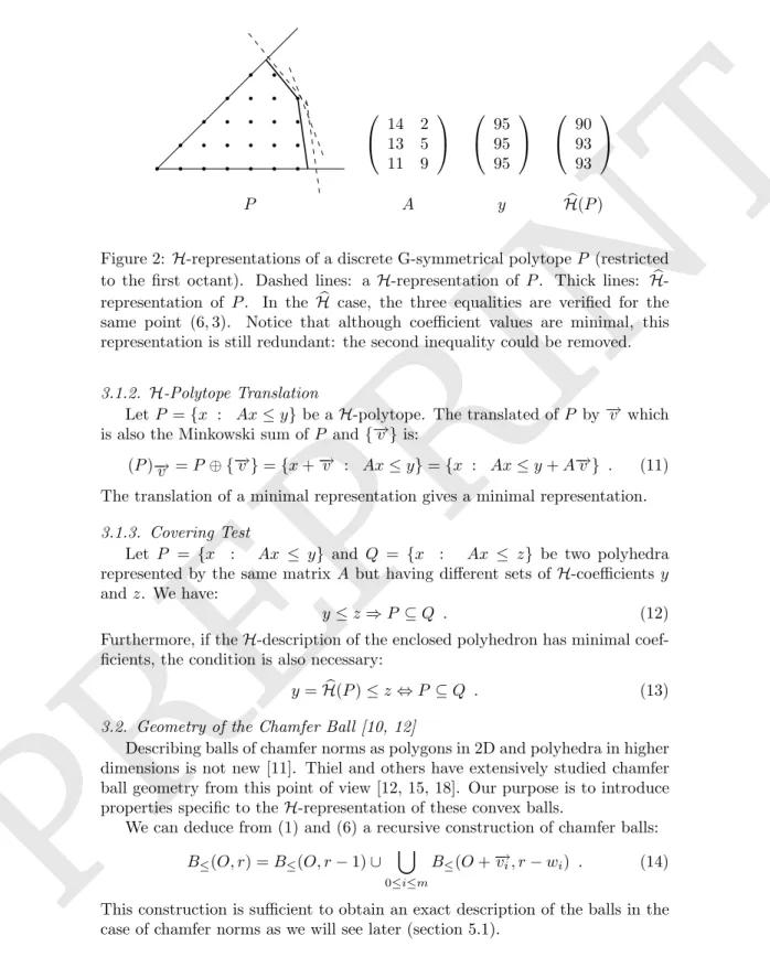
The $H function, introduced for convenience, gives the minimal parameter vector for a given polytope P : $H(P ) = max!Ax : x∈ P". As a consequence, {x : Ax ≤ $H(P )} is the $H-representation of P = {x : Ax≤ y}. Fig. 2
PREPRINT
14 213 5 11 9 9595 95 9093 93 P A y H(P )%Figure 2: H-representations of a discrete G-symmetrical polytope P (restricted to the first octant). Dashed lines: a H-representation of P . Thick lines: %
H-representation of P . In the %H case, the three equalities are verified for the same point (6, 3). Notice that although coefficient values are minimal, this representation is still redundant: the second inequality could be removed.
3.1.2. H-Polytope Translation
Let P = {x : Ax ≤ y} be a H-polytope. The translated of P by −→v which
is also the Minkowski sum of P and {−→v} is:
(P )−→v = P ⊕ {−→v} = {x + −→v : Ax≤ y} = {x : Ax ≤ y + A−→v} . (11)
The translation of a minimal representation gives a minimal representation.
3.1.3. Covering Test
Let P = {x : Ax ≤ y} and Q = {x : Ax ≤ z} be two polyhedra
represented by the same matrix A but having different sets of H-coefficients y and z. We have:
y≤ z ⇒ P ⊆ Q . (12)
Furthermore, if the H-description of the enclosed polyhedron has minimal coef-ficients, the condition is also necessary:
y = %H(P ) ≤ z ⇔ P ⊆ Q . (13) 3.2. Geometry of the Chamfer Ball [10, 12]
Describing balls of chamfer norms as polygons in 2D and polyhedra in higher dimensions is not new [11]. Thiel and others have extensively studied chamfer ball geometry from this point of view [12, 15, 18]. Our purpose is to introduce properties specific to the H-representation of these convex balls.
We can deduce from (1) and (6) a recursive construction of chamfer balls:
B≤(O, r) = B≤(O, r − 1) ∪
&
0≤i≤m
B≤(O + −→vi, r− wi) . (14)
This construction is sufficient to obtain an exact description of the balls in the case of chamfer norms as we will see later (section 5.1).
PREPRINT
Definition 12 (Rational ball). Consider a chamfer mask M, the rational unitary ball or simply rational ball BR is the convex hull of the rational points
− →vi/wi, (−→vi, wi) ∈ M: BR = conv ! −→vi wi : (−→vi; wi) ∈ M " = # m $ i=1 αi − →vi wi : αi∈ R+, m $ i=1 αi= 1 % . (15)
Note that the rational ball, as it is introduced here, is convex by definition and is different, in this regard, from the equivalent rational ball described in [10, 12, 19].
Proposition 1. The homothetic of BR, rBR contains B≤(O, r): B≤(O, r) ⊆
rBR.
Proof. Let p be a point of B≤(O, r) and &m
i=1λi−→vi, λi∈ N be a minimal path
between O and p. Then d(O, p) ≤ r and d(O, p) =&m
i=1λiwi. We can describe
p as a combination of O, r−→v1/w1, . . . , r−v→n/wn:
p = r−d(O,p)r ·O+&mi=1 λiwi r · r wi−→vi, with r−d(O,p) r ≥ 0, λiwi r ≥ 0 ∀i and r−d(O,p) r + &m i=1 λiwi
r = 1. Then, by definition of conv:
p∈ conv(O, r
w1−→v1, . . . ,
r
wn−→vn) ⊂ rBRand every point of B≤(O, r) is in rBR.
Definition 13 (Normal vector [10]). We call normal vector to a facet F of
BR, the unique vector −→F orthogonal to the facet such that ∀p ∈ F, −→F · p = 1.
In the simplicial cone spanned by vectors −→v1
w1 . . . − → vn wn, − →F ·' −→v1 w1 . . . − → vn wn ( = (1 . . . 1). This implies: − →F = (w 1, . . . , wn) · (−→v1| . . . |−v→n)−1 . (16)
The vector α = (−→v1| . . . |−→vn)−1p give the unique representation of p as a
combina-tion of −→v1, . . . , −→vn. If α has integer coefficients then there is a path α(−→v1| . . . |−→vn) to p and its length is (w1, . . . , wn) · α = −→F · p. The normal vector is equivalent
to the elementary displacement and discrete gradient of the cone intercepted by
F as defined for chamfer norms in [10] and [12]. Note that the normal vector is
defined here for general chamfer masks, whether they induce a norm or not. For instance, with the chamfer norm d5,7,11, the point (3, 1) is in the cone
spanned by the vectors −→a = (1 0) and −→c = (2 1) and the weights involved are 5
and 11. The distance between the origin and the point (3, 1) is then [10, (4.32)]:
d(O, (3, 1)) =) 5 11 *· ! 1 2 0 1 "−1 · ! 3 1 " =) 5 1 *·! 31 "= 16 .
PREPRINT
3.3. Mask Conditions for Chamfer NormsProposition 2 (Distance lower bound). If F is a facet of the rational ball and
−
→F its normal vector, then:
d(O, p)≥ −→F · p . (17) Proof. Let p = !iλi−→vi be a minimal path to p, so d(O, p) = !iλiwi. The facet
F is supported by the hyperplane {x ∈ Rn : −→
F · x = 1}. Due to convexity, the
unitary ball is included in the halfspace {x ∈ Rn : −→
F · x ≤ 1}. This applies
to the vertices of the unitary ball −→vi/wi: −→F · −→vi/wi ≤ 1. By linearity of the
dot product, −→F · −→vi ≤ wi and −→F · (!iλi−→vi) = !iλi−→F · −→vi ≤!iλiwi. Hence,
− →F ·!
iλi−→vi is always less than or equal to the length of the path !iλi−→vi.
This lower bound applies for any point p, whether or not it is located in a cone that intercepts F; d does not need to induce a norm.
Proposition 3 (Homegeneity in a unimodular cone). Let CO,U be a unimodular
cone that intercepts a unique facet F of BR. The distance d is homogenous in
the cone and equal to −→F · p, ∀p ∈ CO,U if and only if:
d(O, O + −→u ) = −→F · −→u ,∀−→u ∈ U . (18) Proof. According to proposition 2, d(O, p) ≥ −→F · p, ∀p ∈ CO,U. Since CO,U is
unimodular, p is reachable by a non negative integral combination of vectors of
U , −→Op =!λi−→ui. By triangle inequality and proposition hypotheses, d(O, p) ≤
!λ
id(O, O + −→ui) = ! λi−→F · −→ui = −→F · p. So −→F · p is simultaneously a lower and
upper bound to d(O, p) then the equality holds and d is homogenous in CO,U.
Conversely, consider a vector −→u of U such that d(O, p)'= p · −→F , so d(O, p) > p· −→F , by proposition 2. In the facet F, we always can find n = dim(F) + 1
vertices −→v1/w1. . . −v→n/wn such that −→u lies in the simplicial cone spanned by
the vectors −→v1. . . −→vn. As a consequence −→u can be represented by a unique non
negative combination of n linearly independent vectors: −→u = α· (−→v1| . . . |−→vn).
The components of α = (−→v1| . . . |−→vn)−1· −→u are not necessarily integers (they are
if ∆ ="" det(−→v1| . . . |−→vn)
"
" = 1). However, ∆(−→v1| . . . |−→vn)−1 has integral coefficients
hence ∆−→u can be uniquely represented as an integral combination of the vectors −
→vi: ∆−→u = ∆(−→v1| . . . |−→vn) · α, so there is a path to O + ∆−→u whose length is:
∆(w1. . . wn) · α = ∆(w1. . . wn) · (−→v1| . . . |−→vn)−1· −→u = ∆−→F · p ≥ d(O, ∆−→u ). Thus
d(O, O + ∆−→u ) < ∆d(O, O + −→u ) and the distance is not homogenous in the
cone.
According to this proposition, the homogeneity in a nD unimodular cone can be determined by only testing the vectors of the cone (which are not necessarily in the chamfer mask). We derive a necessary and sufficient condition for norms (a sufficient condition, based on a unimodular triangulation, is given in [10]): Corollary 1 (Norm condition). Let #Ui$be a set of vectors sets Ui with the
PREPRINT
• each unimodular cone Ci= CO,Ui intersects a unique facet of BR;• the union of the cones covers the entire space Zn.
The chamfer mask M induces a norm if and only if: d(O, O + −→u ) = −→F · −→u ,∀−→u ∈!
i
Ui . (19)
Proposition 4 (Direct distance formulation). If d induces a norm, the distance
from O to any point p is:
d(O, p) = max
1≤i≤l
"−→F
i· p# (20)
where l is the number of facets of BR and −→Fi is the normal vector to the ith
facet of BR. This formula does not require to determine in which cone lies p.
Proof. The inequality d(O, p) ≥ −F→i· p holds for all facets due to proposition 2
and the equality d(O, p) = −F→i· p holds, according to proposition 3, for all the
facets of BR (there is at least one of them) that intersect [O, p).
3.4. H-Representation of Chamfer Norm Balls
The H-representation of chamfer balls is directly derived from (20):
p∈ B≤(O, r) ⇔ max
1≤i≤l{−
→
Fi· p} ≤ r ⇔ AM· p ≤ y (21)
where AM is a H-representation matrix depending only on the chamfer mask
M. The number of rows in AM is equal to the number l of facets of BR, each
line of the matrix AM is computed with (16) and y is a column vector whose
values are r. For instance, the H-representation matrix of d5,7,11balls restricted
to G is AM =
$ 5 1
4 3 %
where (5 1) and (4 3) are the normal vectors of the two facets of BR and B≤(O, r) =
& p∈ Zn : $ 5 1 4 3 % · p ≤ $ r r %' . Note that if a polytope is not centered in O, the simplification due to sym-metries do not hold and the full set of H-coefficients is needed, unless we ensure that the H-coefficents for the hyperplanes in the generator G are greater than
H-coefficients for the corresponding symmetric cones. This is the case when a
G-symmetric polytope is translated by a vector in G.
Proposition 5 (Furthest point). Let AM be the matrix defined by a chamfer
mask M generating a norm. The furthest point from the origin in the (H-polytope P ={p : AM· p ≤ (H(P )} is at a distance equal to the greatest component of
(
H(P ).
Proof. By construction of AM, (20) is equivalent to d(O, p) = maxi"AMi· p#,
thus: max p∈P " d(O, p)#= max p∈P "max 1≤i≤l " AMi· p##= max 1≤i≤l" (Hi(P ) # .
PREPRINT
Proposition 6 (Minimal covering ball). The radius of the minimal ball centered
in O that contains all points of a discrete !H-polytope P represented by the matrix AM and the vector !H(P ) is equal to the greatest component of !H(P ).
Proof. The smallest ball that covers the polytope P must contain its furthest
point from the origin:
min"r∈ N : P ⊆ B≤(O, r)#= max
p∈P " d(O, p)#= max 1≤i≤l" !Hi(P ) # .
Definition 14 (Covering function). We call covering function of a set X of points of Zn the function C
X which assigns to each point p of Zn, the radius of
the minimal ball centered in p covering X:
CX: Zn → N
CX(p) = min"r : X⊆ B≤(p, r)# .
The covering function of the chamfer ball B≤(O, r) at point p gives the radius of the minimal ball centered in p that contains B≤(O, r) or, by central symmetry of the chamfer balls, to the radius of the minimal ball centered in O covering
B≤(p, r) and therefore it is the maximal component of the !H-representation of
B≤(p, r):
CB≤(O,r)(p) = max" !H(B≤(p, r)#= max" !H(B≤(O, r)) + AM· p# . (22)
One can notice that the covering function of the zero radius disk is equal to the distance function, as is the distance transform of the complement of this disk:
CB≤(O,0)(p) = DTZn\{O}(p) = d(p, O) = d(O, p) .
Definition 15 (Covering cone). A covering cone Co,U in the covering
func-tion CX is a unimodular cone defined by a vertex o and a set of vectors U, such
that each ball centered in p is included in the ball centered in p + −→u , −→u ∈ U: ∀p ∈ Co,U,∀−→u ∈ U, B≤(p, CX(p)) ! B≤(p + −→u ,CX(p + −→u )) .
Proposition 7. If Co,U is a covering cone in CB≤(O,r) then for any point q in
Co,U \ U \ {o} there exists p such that the ball centered in q includes the ball
centered in p:
B≤(O, r) ! B≤(p, CB≤(O,r)(p)) ! B≤(q, CB≤(O,r)(q)) .
Proof. If U is not empty, there is −→u ∈ U such that p = q − −→u is in Co,U \
{o}. Then, by definition of Co,U, B≤(p, CB≤(O,r)(p)) ! B≤(q, CB≤(O,r)(q)). In
addition, B≤(O, r) ⊆ B≤(p, CB≤(O,r)(p)) always holds by definition of CB≤(O,r).
Proposition 7 is used to limit the search for balls directly covering B≤(O, r)
in the covering function CB≤(O,r). When a covering cone is detected, only its
PREPRINT
Proposition 8. If there is an integer j ∈ [1 . . . l] and a point o such that
AMj· −→ui,∀−u→i ∈ U and !Hj(B≤(o, r)) are maximal then Co,U is a covering cone
in CB≤(O,r).
Proof. Let j be the row number of a maximal component of !H(B≤(o, r)) and
AM· −→ui,∀−→ui∈ U, then j is a maximal component of any positive linear
combi-nation of these vectors. Let p be any point in Co,U, p = o + "iλi−→ui, λi ∈ N.
From (22), we deduce that, in Co,U, CB≤(O,r)takes the form of an affine function
of the components λi: CB≤(O,r)(p) = max # ! H (B≤(o, r)) + $ λiAM−→ui % = H!j(B≤(o, r)) + $ λiAMj−→ui .
In the same way, the radius of the minimal ball centered in p + −→u , −→u ∈ U
covering B≤(O, r) is:
CB≤(O,r)(p + −→u ) = H!j(B≤(o, r)) +
$
λiAMj−→ui+ AMj−→u
= CB≤(p,CB≤(O,r)(p))(O + −→u ) .
In other words, B≤(p, CB≤(O,r)(p)) is contained in B≤(p + −→u ,CB≤(O,r)(p + −→u ))
and Co,U is a covering cone according to definition 15.
4. Triangulation of 3D Chamfer Balls
The first stage of the method consists in decomposing the generator cone
G in unimodular cones that each intercepts a unique facet of the rational ball.
This triangulation has three goals:
1. compute the distance gradients which are vectors normal to the facets of the rational ball. These distance gradients are the rows of the matrix AM;
2. provide a set of unimodular cones suitable for the recursive partition of the generator G used in the next stage;
3. verify that the chamfer mask generates a norm by checking homogeneity in each cone.
4.1. Convex Hull Vertices in the Generator Cone
The expected result is a triangulation of the part of the rational ball BRthat
lies in the generator G. The input data consists in vectors from the chamfer mask
M|G divided by their corresponding weights (to form the equivalent unitary
ball). In the algorithm, these points in Qnare represented as weightings, and all
computations are based on integer arithmetics. The weightings of the chamfer mask are not sufficient alone because:
G&conv' −→vw, (−→v ; w)∈ M
(
%= conv' −→vw, (−→v ; w)∈ M|G
(
PREPRINT
The intersection of BRwith G introduces new vertices that are points in edges of
BRthat intersect the faces of G. This is illustrated in fig. 3a; vectors −→e = (2 1 1)
and −→o = (4 1 1) are not in the chamfer mask and thus can not be vertices of BR,
but they appear in the intersection of BR with (O, {−→a , −→c}). Since the edges
of BR are not known yet, all the intersections of the faces of G with couples
of rational vertices of BR must be added to the input of the algorithm. These
points are rational combinations of the vertices of the intersected edges, but are also represented as weightings with integer coefficients. Among those, the majority of the points that lie in the interior of BRwill be discarded during the
computation of the convex hull.
4.2. Gift-Wrapping Convex Hull and Triangulation of the Rational Ball
Many different algorithms are available for convex hull computation. We chose to implement an modified version of the algorithm known as gift wrapping [20] for two reasons: first it naturally produces a triangulation of the convex hull i.e. a partition in simplicial cones and second, a subpartition of these sim-plicial cones in unimodular cones and the face lattice of the cones can be easily integrated as by-products of the algorithm.
Input: A set of points S
find a starting edge of the convex hull (p, q)
1
push (p, q) in !, the list of active edges
2
while L is not empty do
3 pop (p, q) from ! 4 take r in S \ {p, q} 5 S!← S \ {p, q, r} 6 for s in S! do 7 if s is above (p, q, r) then 8 r← s 9 end 10 end 11
add each newly created edge (r, p) and (q, r) in ! or remove it from !
12
if already contained end
13
Algorithm 1: (Simplified) gift wrapping algorithm [20]
Starting with a first edge, the gift wrapping algorithm (1) iteratively extends the convex hull by appending a new triangle and its edges. Since the convex hull is computed in G, one vertex of the starting edge can be chosen as the point in the first axis of G that is closest to the origin: p = (x1, 0, 0) (with maximal
x1 if several points exist on this axis) and the second vertex is the point q
that maximizes the angle (O, p, q) in a facet of G containing p. The algorithm proceeds until exhaustion of active edges.
PREPRINT
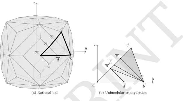
− →c − →e − →o − →b − →d − →a z x y(a) Rational ball
− →a −→b − →c − →d − →e − →o − →h z y (b) Unimodular triangulation
Figure 3: The rational ball BR of the 3D chamfer mask 7,8,11,14 and a
uni-modular triangulation of BR∩ G. (b) Unimodular triangulation in 3D cones
(represented by triangles) of BR∩ G (thick lines in (a)). Each Z3 point (x, y, z)
is projected onto (y/x, z/x) (Farey space).
{!e,!h} {!b,!h, !o} {!b, !e} G {!c, !e} {!a, !d} {!b, !d, !o} {!a, !d, !o} {!b, !d} {!d, !o} {!b, !o} {!b,!h} {!b, !c} {!b, !e,!h} {!a, !o}
{!a} {!d} {!o} {!b} {!h} {!e} {!c}
{!b, !c, !e}
∅ {!h, !o}
Figure 4: Lattice of cone vector sets for the unimodular triangulation of BR∩ G
PREPRINT
4.3. Unimodular triangulationThe gift wrapping algorithm produces a set of nD simplicial cones Co,U, each
of which is unimodular if and only if det(U) = ±1. When | det(U)| > 1, a new point is introduced as an input of the convex hull computation and the detected non unimodular cone is discarded. The unimodular triangulation is represented by a cone lattice L used later as a partition of G.
The intersection of the rational ball for mask 7,8,11,14 and G is pictured in fig. 3b. A unimodular triangulation without any new point of the face (−→b =
(1 1 0), −→d = (2 1 0), −→e = (2 1 1), −→o = (4 1 1)) can not be made because
det(−→d , −→e , −→o ) = det(−→b , −→e , −→o ) = 2. This is solved by introducing the vector −
→h . The cone lattice corresponding to this unimodular triangulation is pictured
in fig. 4.
4.4. Homogeneity check
The unimodular triangulation of BR produces a set of cones that cover the
generator G and their corresponding face normal vectors. Using corollary 1, by comparing d(O, O + −→u ), obtained by propagating the chamfer weights, with −
→
Fi· −→u , where −→F is the normal vector of one of the faces that intersects [O, −→u ),
we determine if the distance is homogenous in G, so by symmetry, in Z3.
5. LUT and Test Neighborhood Computation for 3D chamfer norms
5.1. !H-Representation of Chamfer Balls
The computation of the LUT is based on a !H-representation of the chamfer
norm balls. All share the same matrix AM which depends only on the chamfer mask (21). The !H-coefficients of the balls are computed iteratively from the ball of radius 0, B≤(O, 0) ="x : AMx = 0#using (14) and (11):
!
H(B≤(O, r)) = max" !H(B≤(O, r − 1)); !H(B≤(O, r − wi)) + AM−→vi, i∈ [1..m]# .
5.2. LUT values
LUT values are directly obtained from the covering function (22): Lut−→vi[r] = 1 + CB≤(O,r−1)(O + −→vi) = 1 + max" !H(B≤(O, r − 1)) + AM· −→vi
#
. 5.3. Test neighborhood
The algorithm 2 begins with an empty test neighborhood T and seek direct covering relations in balls of increasing radii like the method in [7]. However, in [7], the covering relations are seen from the perspective of the covering balls (in the distance map, requiring propagation of distances), whereas in our case, they are considered from the point of view of the covered balls, i.e. in the covering function that can be computed directly without propagation using the direct formula (22). The algorithm uses the lattice of cones L (fig. 4), resulting from the triangulation phase, as a partition of G. Each cone that is not a covering
PREPRINT
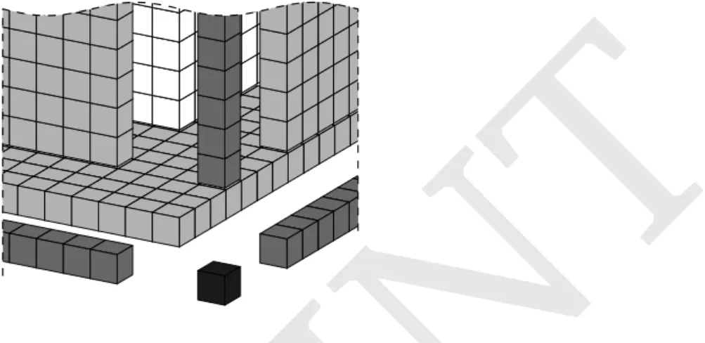
Figure 5: The partition of a 3D unimodular cone in 23 subcones (from darkest
to lightest): 1 point, C3
1 = 3 1D cones, C23= 3 2D cones and C33= 1 3D cone.
cone is recursively partitioned by procedure visitCone as depicted in fig. 5: a
nD cone Co,U is divided in 2n subcones corresponding to all the subsets of U.
Direct covering relations at the vertices of all the visited cones are checked by procedure visitPoint using a direct computation of the covering function in all know neighbors in T .
Input: L lattice of simplicial unimodular cones, maximal radius R
T ← ∅;
1
for r ← 1 to R do // inner radius
2
foreach CO,U ∈ L do // cones with increasing dimension
3 o← O +!−→u∈U−→u ; 4 visitCone(T , Co,U, r); 5 end 6 end 7
Algorithm 2: Computation of the test neighborhood
6. Results
An implementation of these algorithms was developed in the C language. It produces output in the same format as the reference algorithm [7] so that outputs can be compared character-to-character. Tests were done on various chamfer masks and different maximal radii and helped discover a propagation issue in the reference algorithm. This problem corrected, the results are almost always identical except for insignificant cases close to the maximal radius for which covering radii exceed the maximum. These radii are handled differently by both algorithms but since they exceed the maximum radius, there is no impact on the medial axis computation.
PREPRINT
Input: T , Co,U, inner radius r, y = !H(B≤(o, r))
visitPoint (o)
1
// Visit subcones if Co,U is not a covering cone
if ∀j, ∀−→u ∈ U : yj %= maxk"yk#and AMj· −→u %= maxk"AMk· −→u#then
2
foreach subcone Co,U! of Co,U do
3 o"← o +$−→ u∈U!−→u ; 4 visitCone(T , Co!,U!, r); 5 end 6 end 7
Procedure visitCone(T , Co,U, r)
Input: T , inner radius r, ball center p to test
if ∀−→v ∈ T : B≤(O + −→v ,CB≤(O,r)(O + −→v ))%⊂ B≤(p, CB≤(O,r)(p)) then 1 T ← T ∪"−→Op# 2 end 3 Procedure visitPoint(T , r, p)
The run times of both reference and proposed algorithms are given in table 1 for various sizes and a few masks. These figures show that the overall mean computational complexity is linear with the maximal radius for the proposed method whereas it is of order r4 in 3D for the reference algorithm.
Table 1: Run times (in seconds) of reference (ref.) and proposed (H) method implementations for four 3D masks and various volume sizes L × L × L.
3, 4, 5 3, 4, 5, 7 7, 8, 11, 14 4, 6, 7, 9, 10
L ref. H ref. H ref. H ref. H
10 0.0006 0.0003 0.0002 0.0004 0.0013 0.0010 0.0004 0.0008 20 0.0049 0.0002 0.0032 0.0004 0.0135 0.0011 0.0047 0.0010 50 0.1079 0.0003 0.1096 0.0005 0.2886 0.0027 0.1592 0.0015 100 1.6316 0.0005 1.6831 0.0008 4.4704 0.0054 2.4626 0.0023 200 30.391 0.0010 31.126 0.0012 81.627 0.0109 53.126 0.0038 500 3523 0.0022 3537 0.0024 9333 0.0272 6465 0.0088 1000 0.0042 0.0073 0.0549 0.0220 7. Conclusion
In this paper, methods to compute both the chamfer LUT and the test neighborhood were presented. Speed gains from the reference algorithm [7] are attributable to the representation of chamfer balls as H-polytopes. With this description, we avoid the use of weight propagation in the image domain and
PREPRINT
obtain a constant time covering test by the direct computation of covering radii. Moreover the search space is greatly reduced using covering cones.
While applications always using the same mask can use precomputed test neighborhood T and LUT, other applications that potentially use several masks, adaptive masks, variable input image size can benefit from these algorithms. A faster computation of T is also highly interesting to explore chamfer mask properties. Beyond improved run times, the H-polytope representation helped to prove new properties of chamfer masks. And a new formula of distance which doesn’t need to find in which cone lies a point was given.
Examples and source codes for the 3D and 2D cases are available by simple email request to the authors or in the code section of the IAPR-TC18 web site (http://www.cb.uu.se/~tc18/).
Acknowledgment
The authors would like to thank the referees for their valuable suggestions and comments, which greatly improved the paper.
References
[1] A. Rosenfeld, J. L. Pfaltz, Sequential operations in digital picture process-ing, Journal of the ACM 13 (4) (1966) 471–494. doi:10.1145/321356. 321357.
[2] U. Montanari, A method for obtaining skeletons using a quasi-euclidean dis-tance, Journal of the ACM 15 (4) (1968) 600–624. doi:10.1145/321479. 321486.
[3] G. Borgefors, Distance transformations in arbitrary dimensions, Computer Vision, Graphics, and Image Processing 27 (3) (1984) 321–345. doi:10. 1016/0734-189X(84)90035-5.
[4] D. Coeurjolly, A. Montanvert, Optimal separable algorithms to compute the reverse Euclidean distance transformation and discrete medial axis in arbitrary dimension, IEEE Transactions on Pattern Analysis and Machine Intelligence 29 (3) (2007) 437–448. doi:10.1109/TPAMI.2007.54.
[5] R. Strand, Weighted distances based on neighborhood sequences, Pattern Recognition Letters 28 (15) (2007) 2029–2036. doi:10.1016/j.patrec. 2007.05.016.
[6] G. Borgefors, Centres of maximal discs in the 5-7-11 distance transforms, in: Proc. 8th Scandinavian Conf. on Image Analysis, Tromsø, Norway, 1993, pp. 105–111.
[7] ´E. R´emy, ´E. Thiel, Medial axis for chamfer distances: computing look-up tables and neighbourhoods in 2D or 3D, Pattern Recognition Letters 23 (6) (2002) 649–661. doi:10.1016/S0167-8655(01)00141-6.
PREPRINT
[8] N. Normand, P. ´Evenou, Medial axis LUT computation for chamfer norms using H-polytopes, in: Discrete Geometry for Computer Imagery, Vol. 4992 of LNCS, Springer Berlin / Heidelberg, 2008, pp. 189–200. doi:10.1007/ 978-3-540-79126-3_18.
[9] A. Rosenfeld, J. Pfaltz, Distances functions on digital pictures, Pattern Recognition Letters 1 (1) (1968) 33–61. doi:10.1016/0031-3203(68) 90013-7.
[10] ´E. Thiel, G´eom´etrie des distances de chanfrein, m´emoire d’habilitation `a diriger des recherches, Universit´e de la M´editerran´ee, Aix-Marseille 2, http://www.lif-sud.univ-mrs.fr/~thiel/hdr/ (Dec. 2001).
[11] B. J. H. Verwer, Local distances for distance transformations in two and three dimensions, Pattern Recognition Letters 12 (11) (1991) 671–682. doi: 10.1016/0167-8655(91)90004-6.
[12] ´E. R´emy, Normes de chanfrein et axe m´edian dans le volume discret, Th`ese de doctorat, Universit´e de la M´editerran´ee (Dec. 2001).
[13] C. Arcelli, G. Sanniti di Baja, Finding local maxima in a pseudo-Euclidian distance transform, Computer Vision, Graphics, and Image Processing 43 (3) (1988) 361–367. doi:10.1016/0734-189X(88)90089-8.
[14] S. Svensson, G. Borgefors, Digital distance transforms in 3D images us-ing information from neighbourhoods up to 5×5×5, Computer Vision and Image Understanding 88 (1) (2002) 24–53. doi:10.1006/cviu.2002.0976. [15] ´E. Thiel, Les distances de chanfrein en analyse d’images : fondements et applications, Th`ese de doctorat, Universit´e Joseph Fourier, Grenoble 1, http://www.lif-sud.univ-mrs.fr/~thiel/these/ (Sep. 1994). [16] ´E. R´emy, ´E. Thiel, Computing 3D medial axis for chamfer distances, in:
Discrete Geometry for Computer Imagery, Vol. 1953 of LNCS, Uppsala, Sweden, 2000, pp. 418–430. doi:10.1007/3-540-44438-6_34.
[17] G. M. Ziegler, Lectures on Polytopes (Graduate Texts in Mathematics), Springer, 2001.
[18] G. Borgefors, Weighted digital distance transforms in four dimensions, Discrete Applied Mathematics 125 (1) (2003) 161–176. doi:10.1016/ S0166-218X(02)00229-9.
[19] C. Fouard, G. Malandain, 3-D chamfer distances and norms in anisotropic grids, Image and Vision Computing 23 (2) (2004) 143–158. doi:10.1016/ j.imavis.2004.06.009.
[20] D. R. Chand, S. S. Kapur, An algorithm for convex polytopes, Journal of the Association for Computing Machinery 17 (1) (1970) 78–86. doi: 10.1145/321556.321564.