Design and Transformation of Three Dimensional
Pupils: Diffractive and Subwavelength
by
Hanhong Gao
B.S., Peking University (2009)
S.M., Massachusetts Institute of Technology (2011)
Submitted to the Department of
Electrical Engineering and Computer Science
in partial fulfillment of the requirements for the degree of
Doctor of Philosophy in Electrical Engineering and Computer Science
at the
MASSACHUSETTS INSTITUTE OF TECHNOLOGY
June 2014
c
⃝ Massachusetts Institute of Technology 2014. All rights reserved.
Author . . . .
Department of
Electrical Engineering and Computer Science
May 21, 2014
Certified by . . . .
George Barbastathis
Professor of Mechanical Engineering
Thesis Supervisor
Accepted by . . . .
Leslie A. Kolodziejski
Chair, Department Committee on Graduate Students
Design and Transformation of Three Dimensional Pupils:
Diffractive and Subwavelength
by
Hanhong Gao
Submitted to the Department of Electrical Engineering and Computer Science
on May 21, 2014, in partial fulfillment of the requirements for the degree of
Doctor of Philosophy in Electrical Engineering and Computer Science
Abstract
Three dimensional pupils are investigated in both diffractive and subwavelength regimes and in various applications to shape the flow of light. In diffractive regime, volume holograms are good candidates for pupils of optical imaging systems thanks to their three–dimensional structure, which provides richer design flexibility compared to conventional two–dimensional pupils. In this thesis, I will propose the system design as well as the optimization of depth selectivity for enhancing the signal–to–noise ratio of ground–based imaging system for the detection of artificial satellites. In addition, deformations of volume hologram pupils promise additional opportunities to design further, more sophisticated point spread functions which are potentially useful for many imaging purposes. Deformations using multiple point indenters will be investi-gated in terms of both forward and inverse problems. Bulk transformation is a more general approach for pupil design. The physical relationship between transformation and resulting point spread function will be discussed by deriving the correspond-ing analytical expressions. In subwavelength regime, I will explore the realization of key materials properties including inhomogeneity and anisotropy. Anisotropy can be implemented by elliptical rod lattices; and with anisotropy, cloaking and accommo-dation of different components of an optical device become possible. Inhomogeneity is discussed in the context of gradient–index media. The additional thin–film wave guidance effect along the third dimension due to fabrication constraints is investigat-ed in detail with the proposal of an all–analytical solution.
Thesis reader: Leslie A. Kolodziejski, Professor of Electrical Engineering, MIT Thesis reader: Michael R. Watts, Associate Professor of Electrical Engineering, MIT Thesis Supervisor: George Barbastathis
Acknowledgments
First and foremost, I would like to thank the “lovely” 3D Optical Systems Group. You rock! Especially, I would like to thank my thesis advisor, Professor George Barbastathis, for his patient guidance and support for my research. He is very nice and is definitely a great professor. His instructions and suggestions have been extremely thought–provoking. Just like magic, his suggestions are especially helpful when I was stuck or struggling with difficulties. Also, I enjoy his jokes, admire his talent of languages and his ambition & vast progress in learning “one of the most difficult languages on Earth”. I also thank him for teaching me how to pronounce correctly, write professionally, avoid common mistakes, and make fun/jokes in English.
I also appreciate the help, suggestion and criticisms from my committee members, Professor Leslie Kolodziejski and Professor Michael Watts. They offered great advice, and provided me with right paths towards my thesis. I thank for their patience when I had to routinely bother them to check their calendars and make my committee meetings and defense happen. I am also grateful to Professor Steven Johnson. His criticisms on my thin–film metamaterials project have been very useful. My appre-ciation extends to Professor Tom´as Palacios as well, who, as my academic counselor, oversaw my PhD process and asked me to enjoy “the best time of your life.”
As for our “3DOSG”, I am very grateful to my nice, cute and supportive colleagues (past and present, MIT and Singapore) for their useful discussions, comments and kind help from every aspect: Disi A, Aditya Bhakta, Dipanjan Bhattacharya, Chih-Hao Chang, Wensheng Chen, Zhi Chen, Seongkeun Cho, Hyungryul Johnny Choi,
Martin Deterre, Sagrario Dominguez, Jos´e A. Dominguez-Caballero, Yubo Duan,
Chih-Hung Max Hsieh, Howard Yuanhao Huang, Hyun-Jin In, Jeong-gil Kim, Jason Ku, Justin Lee, Xiaogang Larry Liu, Yi Liu, Nick Loomis, Yen-Sheng Lu, Yuan Luo, Qin Miao, Anthony Nichol, Se Baek Oh, Adam Pan, Jon Petruccelli, Shakil Rehman, Nader Shaar, Yongjin Sung, Satoshi Takahashi, Chee Wee Tan, Kehan Tian, Lei Tian, Nikhil Vadhavkar, Laura Waller, Renze Wang, Jon Watson, Hongyi Xu, Kelli Xu, Se Young Yang, Baile Zhang, Zhengyun Zhang, and Yunhui Zhu. Among them,
I would especially thank Lei and Yi for suggestions and discussions on how to handle different research topics and the future, thank Zhi for lessons on experiments, Max and Satoshi for discussions on nanophotonics and fabrication, Jon (Jonathan Watson) and Scott (J. Scott Stuart) from Lincoln Laboratory for guidance and suggestions on the satellite project, Baile for helping in electromagnetics, Nick for computing guidance and American culture lessons, Laura for help on nonlinear optics, Se Baek and Jon for guidance in phase space optics, and our lovely Singapore crew (Yubo, Zhi, Zhengyun, Wensheng, and Hongyi) for offering me a place to stay. I also thank Irina Gaziyeva, Tuyet-Mai Hoang, Adiana Abdullah and Jaseema Abdul Karim for their help on paperworks and reimbursements. I appreciate the efforts from MIT International Students Office and Singapore’s SMART headquarters on maintaining my legal status in both the United States and Singapore.
Last but not the least, I would thank my wife, Yue Wu. Being a spouse of a PhD student is definitely no easy task. This thesis would not be possible without her love, consideration and support. I would also like to thank my parents and parents-in-law for their support and love.
Contents
1 Introduction 21
1.1 Volume holograms – 3D diffractive pupils . . . 22
1.1.1 VH for satellite detection in daytime . . . 26
1.1.2 PSF design: multiple point indenters . . . 28
1.1.3 PSF design: transformational volume holography . . . 29
1.2 Subwavelength metamaterials . . . 30
1.2.1 Cloaking in subwavelength regime: anisotropy . . . 31
1.2.2 Thin–film gradient index subwavelength metamaterials: inho-mogeneity . . . 32
1.3 Outline of the thesis . . . 34
2 Volume holographic filters for mitigation of daytime sky brightness in satellite detection 37 2.1 VHF system design . . . 38
2.2 Telephoto objective . . . 39
2.3 Analysis methodology . . . 41
2.4 Mitigation of daylight due to longitudinal defocus . . . 42
2.5 Multispectral issue and performance analysis . . . 43
2.6 The SNR and design parameters . . . 46
2.7 Discussion of multi–pixel cameras . . . 49
2.8 Field of view (FOV) . . . 51
2.9 Aberrations . . . 52
2.11 Experiment . . . 60
2.11.1 Experimental geometry . . . 60
2.11.2 Result: Case I . . . 61
2.11.3 Result: Case II . . . 62
2.11.4 Result: Case III . . . 63
2.12 Conclusion . . . 63
3 Design of volume holographic point spread functions using point deformations 65 3.1 From single to multiple point deformations . . . 66
3.2 Continuous force . . . 69
3.3 Multiple point deformations: examples . . . 70
3.4 Inverse problem: optimization . . . 70
3.5 Inverse problem: examples . . . 73
3.6 Conclusion . . . 75
4 Transformational volume holography 77 4.1 Volume holographic imaging systems . . . 78
4.2 Transformation analysis . . . 79 4.3 Affine transformations . . . 81 4.3.1 Hologram shrinkage . . . 81 4.3.2 Compression . . . 83 4.3.3 Rotation . . . 84 4.3.4 Shearing . . . 85 4.4 Non–affine transformations . . . 87 4.4.1 Bending . . . 87
4.4.2 Stationary phase method . . . 89
4.4.3 Twisting . . . 95
5 Subwavelength dielectric photonic cloak 103 5.1 Motivation . . . 104 5.2 Implementation of anisotropy with elliptical rods . . . 105
5.3 Cloaking and accommodating examples . . . 106
5.3.1 Accommodation of peripheral non–photonic components . . . 106
5.3.2 Accommodation of internal non–photonic components . . . 108
5.4 Gradient–index antireflection layers . . . 109 5.5 Conclusion . . . 111
6 Thin–film subwavelength L¨uneburg lens 119
6.1 Analytical method for effective refractive index estimation . . . 121
6.1.1 Effective guiding medium (EGM) method . . . 122
6.1.2 Relationship between effective refractive index and rod radius 126
6.2 Corrected design of the subwavelength L¨uneburg lens . . . 128 6.3 Anisotropic guidance correction . . . 129 6.4 Conclusion . . . 135
List of Figures
1-1 (Left) Setup for volume hologram recording process. (Right) Example
of recorded permittivity distribution on the hologram when θs=−θf. Color shading denotes the value of permittivity (see Eq. 1.4). . . 24 1-2 Setup for probing of recorded volume holograms. . . 25 1-3 Two types of subwavelength metamaterial lattices. Black dots are rods
of certain material, e.g. silicon, and white ambient is other material, e.g. air. Red dashed lines highlight the corresponding unit cell of the lattice. . . 33 1-4 (a) Structure of designed subwavelength aperiodic nanostructured L¨uneburg
lens under 2D assumption. (b) Finite–difference time–domain simula-tion and ray tracing simulasimula-tion results. Red circle outlines the edge of the L¨uneburg lens and blue curves are ray tracing results. Black dots are silicon rods of infinite height (thus 2D assumption) immersed in air. Color shading denotes the field of the wave propagating through this subwavelength lens. . . 35
2-1 VHF design architecture. As an example, this VHF is assumed to
be used for Iridium satellite detection. Inset: a typical diffraction efficiency plot with respect to longitudinal defocus δ. . . . 38
2-2 (top) VHF system architecture using a telephoto as objective, and
(bottom) its effective configuration. PP1: first principal plane. . . 40
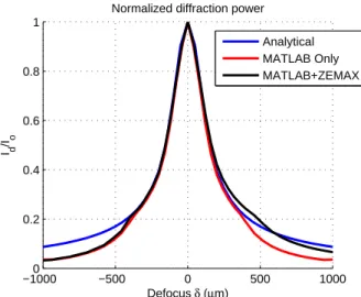
2-3 Comparison of three computational methods for a simple VHF system
2-4 Diffraction efficiency of atmospheric scatterers for VHF system de-signed for Iridium satellite detection, calculated used analytical method
(left) and MATLAB+ZEMAX method (right). . . 42
2-5 Diffraction efficiency of atmospheric scatterers for Geosynchronous
de-tection VHF system architecture, calculated used analytical method
(left) and MATLAB+ZEMAX method (right). . . 43
2-6 (a) Radiance of daylight scattering at different altitudes, (b) spectral radiance of the sky background at ground level, and (c) solar spectral irradiance. All figures are calculated using MODTRAN 4 [113] assum-ing 23 km ground visibility and rural extinction haze model. The angle was 10 degrees east of zenith at 3:00 PM local time on June 21 at 45
degrees latitude (mid–latitude summer atmospheric model). . . 45
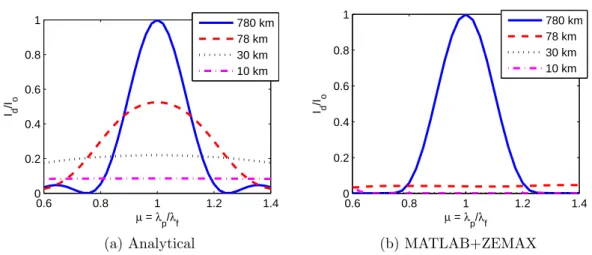
2-7 Multispectral performance of the VHF system for probe source at
dif-ferent altitudes, calculated using (a) analytical method and (b)
MAT-LAB+ZEMAX method. . . 46
2-8 (a) Signal diffraction efficiency, (b) noise diffraction efficiency, and (c) total system SNR enhancement with respect to hologram thicknesses and recording angles. . . 49 2-9 (a) Diffraction efficiency for satellites at different altitudes, when the
system is solely designed for detection of Iridium satellites. Diffraction efficiency (Id/I0) is normalized to the readout intensity when the
holo-gram is probed by Iridium satellites. (b) Turbulence–free point spread functions at multi–pixel cameras for satellites at different orbit heights. From left to right, top to bottom: Sputnik-1 (215 km), International Space Station (340 km), Hubble Space Telescope (595 km), and Irid-ium (780 km). Color shading denotes the normalized intensity. Note that different axes are used for these four pattern plots. . . 51 2-10 (a) Illustration of FOV along y direction; (b) Angle detuning along x
direction. . . 52
2-12 Diffraction efficiency at different longitudinal defocus for each type of aberration. Red curves are cases without aberration and blue curves are with aberration. The following values are used for the coefficient of each aberration: spherical aberration B = 100, astigmatism C = 2× 10³, curvature of field D = 5× 10³, distortion E = 1× 10⁴, and
comma F = 50. . . . 54 2-13 (Top) Diffraction efficiency of objects at various altitudes for our VHF
system considering spherical aberration (left) and astigmatism (right). Blue curves are without aberration, red and black curves are with aberration of different signs. (Bottom) Zoomed–in view of top row for objects with height below 30 km. Spherical aberration coefficients
are chosen as B = 10 and B = −10, and astigmatism coefficients are
chosen as C = 4× 10² and C =−4 × 10². . . . . 55
2-14 Typical Zernike polynomials. When they are weighted by certain co-efficients for each polynomial term, their summation gives the phase profile of atmospheric turbulence. . . 56 2-15 Examples of phase profiles for atmospheric turbulence at different
val-ues of FWHM of astronomical seeings. . . 58 2-16 Examples of point spread functions at the detector when probed by
signal beams without defocus, for atmospheric turbulence at different values of FWHM of astronomical seeings. . . 59 2-17 Diffraction efficiency of objects at various altitudes for our VHF system
considering atmospheric turbulence at different values of astronomical seeings. Left figure shows the entire range from 0 to 780 km, right figure is a zoomed–in at the altitudes of atmospheric scatterers from 0 to 30 km. . . 59 2-18 Scale down experimental geometry. BS: Beamsplitter, L1: Positive
2-19 (Left) Images from the conventional system (top, Camera 1) and the VHF system (bottom, Camera 2), with illumination from both satel-lite (monochromatic) and daylight (broadband). (Right) Line profile across the signal spot for both images. . . 62 2-20 (a) Contrast ratio comparison of the conventional and VHF systems
with only satellite. (b) Contrast ratio comparison of the conventional and VHF system with both satellite and daylight. (c) Rate of contrast decrease after introducing daylight. (d) Images at detectors for the conventional (i) and VHF (ii) system with only satellite, as well as the conventional (iii) and VHF (iv) system with both satellite and daylight. 64
3-1 (a) Fourier geometry of reflection volume hologram. (b) PSF of
geom-etry (a) with and without the point load. . . 67
3-2 (a) Imaging system geometry utilizing a reflection volume hologram.
(b) Illustration of VH deformations with multiple point indenters. . . 68 3-3 Approximation of a continuous force using discrete point indenters, or
vice versa. . . 69 3-4 (a)(b)(c) Three different kinds of desired PSFs normalized to the peak
intensity of the PSF without deformation at Bragg matched probe beam θp = 172◦. (d)(e)(f) Combination of point loads to achieve the above PSFs, and the corresponding fringe patterns. Red dashed lines and blue solid lines denote the pattern before and after the deforma-tion, respectively. (g)(h)(i) Angle detuning Bragg mismatched PSFs. The brightness plotted is the normalized intensity. . . 71 3-5 (Left) Designed PSFs, (middle) combinations of point loads, and (right)
the corresponding fringe patterns for a shifted PSF. For fringe pattern plots, red dashed lines and blue solid lines denote the pattern before and after the deformation, respectively. . . 73
3-6 (Left) Designed PSFs, (middle) combinations of point loads, and (right) the corresponding fringe patterns for: (from top to bottom) wide angular PSF (Case I), wide rectangular PSF (Case II), narrow rect-angular PSF. For fringe pattern plots, red dashed lines and blue solid lines denote the pattern before and after the deformation, respectively. 74 3-7 (Left) Designed PSFs, (middle) combinations of point loads, and (right)
the corresponding fringe patterns for (top) PSF with narrowed main lobe, and (bottom) PSF with suppressed side lobes. For fringe pattern plots, red dashed lines and blue solid lines denote the pattern before and after the deformation, respectively. . . 75
4-1 Two analysis approaches for including bulk transformations in volume
holographic imaging systems. For each case, left and right figures show coordinates used for calculating the integrals without and with the transformation, respectively. . . 80 4-2 (Left) Shrinkage of the VH along (a) z′′ and (c) x′′ directions. (Right)
The resulting PSFs when the compression ratio (b) δ = 0.1 & (d)
δ = 0.02, respectively. . . . 83
4-3 (a) Rotation of the VH and (b) the resulting PSF when the rotation
angle θ = 2o calculated using both derived analytical equations and direct full numerical solution. . . 85 4-4 (a) Shearing of the VH along x′′ direction and (b) the resulting PSF
when the shearing ratio α =−0.04. . . . 86
4-5 (a) Bending of the VH. (b) Resulting PSFs at different bending ratios. 87
4-6 PSFs calculated using Eq. 4.32 by including the contributions (a) only poles and (b) both poles & boundaries, compared with full numerical solution. . . 91
4-7 Expressions of f (x) (left), Λϕ(x) (middle) and real(exp(iΛϕ(x)))(right) for one dimensional integral of Eq. 4.24 at detector positions of x′ = 0 (top), x′ =−3.2 × 10⁻⁴ m (middle), and x′ =−3.1 × 10⁻⁴ m (bottom) (see Fig. 4-6). Note that only part of the integral range is shown. . . 92
4-8 PSF at the detector for a bent hologram calculated using stationary
phase approximation combining four critical points, compared with full numerical solution. . . 95
4-9 (a) PSFs calculated from Part 1–3 and combined. (b)–(d)
Contribu-tions from Part 1–3 separately. . . 96
4-10 PSFs for twisting at different maximum twisting angles: (a) θm = 0o (without deformation), (b) θm = 0.5o, and (c) θm = 1o. Note that in order to show sidelobes clearly, √q(x′, y′) is plotted instead of the actual intensity, which is proportional to |q(x′, y′)|2. . . . 97
4-11 Intuitive explanation of the PSF shape after twisting. . . 98
4-12 Approximation of jinc function (Eq. 4.50). . . 100
4-13 (a) PSF calculated using stationary phase method approximation, and (b) its difference to the result calculated using full numerical result (Fig. 4-10(b)). Maximum twisting angle is θm= 0.5o. . . 101
5-1 Illustration of accommodating mechanical components into photonic
5-2 Elliptical (a) and circular (b) silicon rod lattice structure. Isofrequency diagrams of silicon elliptical (c) and circular (d) rod unit cells, where only the first TM band is shown. The size of the unit cell is a× a. The long and short axes of the elliptical rod in (a) are 0.95a and 0.5a, respectively; the radius of circular rod in (b) was chosen as 0.294a to match the effective index of the isotropic circular rod case with the effective value of the index along the x axis in the anisotropic elliptical rod case. Labels on the lines denote the corresponding normalized frequency ωa/2πc. The bold blue lines correspond to the free space wavelength λ = 8a used in this thesis. . . . 112
5-3 Space transformation of the first design example. More peripheral
area (green) for accommodating mechanical components is created by squeezing the uniform medium into an anisotropic medium. Blue ar-rows are ray trajectories, and red lines illustrate wavefronts. . . 113
5-4 (a)(b) Original structure and the structure of the first design example. Blue boxes are the zoomed–in view of the lattices. Red lines denote the interfaces between different media: PEC, isotropic and anisotropic medium. (c)(d) FDTD results of original structure and accommodating design. Illumination is TM Gaussian source with incident angle of 45◦. Black stripe is PEC and green stripe is area for accommodating mechanical components. Color shading denotes the magnetic field (Hz) distribution. Red is positive and blue is negative. . . 114
5-5 Transformation of space to create a parallelogram for accommodating
internal mechanical components. Ray tracing results are illustrated.
5-6 Structure of the second design example, composed of uniform elliptical and circular silicon rod arrays. Grey parallelogram in the middle is region for mechanical components and magenta arrows are the optical axes of the anisotropic media. The dimensions are D = 50a = 6.25λ,
α = 38.5◦ and β = 13.3◦. Note that this implementation is for proof– of–concept and is definitely scalable. . . 115 5-7 FDTD simulation results of this design illuminated by plane wave with
λ = 8a at time t = 6.25λ/c, 12.5λ/c, 18.75λ/c, 25λ/c, respectively.
Color shading denotes the magnetic field (Hz) distribution, where red is positive and blue is negative. . . 116 5-8 Amount of reflection and scattering for diamond–shape cloak (Fig. 5-6)
at different cloaking sizes (β angles) in (a) linear and (b) logarithmic scale. . . 117 5-9 One example of gradient–index antireflection layers, where four layers
are used. . . 117 5-10 FDTD simulation results and sampled ray tracing of the photonic cloak
without (a) and with (b) gradient–index antireflection layers. Ray tra-jectories for (a) are duplicated (black arrows) in (b) as a comparison to the trajectories for (b) (light blue arrows), illustrating the resulting lateral shift. Green lines illustrates the boundary or antireflection lay-ers between circular and elliptical rod lattices. Color shading denotes the magnetic field [Hz] distribution. . . 117 5-11 Reflection coefficient (a) and lateral shift (b) with respect to the
num-ber of antireflection layers for different incident angles. Negative value for the lateral shift means a shift to negative–x direction from the correct position. . . 118
6-1 (a) Finite height rod lattice structure. (b) 2D rod lattice structure assuming infinite height. . . 121
6-2 Effective guiding medium (EGM) approximation of 2D finite height rod lattice structure. . . 122
6-3 Graphical solutions of wave guidance condition [Eq. (6.6) and (6.7)] for TE (a) and TM (b) polarizations. Blue and red lines are the left and right hand sides of these equations, respectively. Operating frequencies
ω1 = 0.11× 2πc/a, ω2 = 0.16× 2πc/a, ω3 = 0.14× 2πc/a and ω4 =
0.18× 2πc/a. Rod radius r = 0.50a. . . 124
6-4 (a) The supercell used in the DBD method for the finite height rod
lattice structure. (b) Isofrequency contour of the supercell with r = 0.50a where the first band only is shown. Labels on the lines denote the corresponding normalized frequency ωa/2πc. The bold blue line corresponds to the wavelength λ = 6a used in this chapter. (c) Field distribution of the waveguide slab at a particular x slice. Color shading denotes magnetic field (Hy) distribution and black contours illustrate silicon rods. . . 125
6-5 (a) Comparison between the dispersion relation for finite–height silicon rod lattice [Fig. 6-1(a)] calculated from the EGM and DBD method, and the dispersion relation for infinite–height 2D rod lattice [Fig. 6-1(b)]. For each case, the two lowest bands representing the TM and TE modes are shown. (b) Relationship between effective refractive index and rod radius calculated from both methods, compared with the relationship for infinite–height 2D rod lattice. Free space wavelength of light is λ = 6a = 1550 nm. . . . 127
6-6 Relationship between calculated effective refractive index and height
6-7 (a) Top view and side view of the thin–film subwavelength L¨uneburg lens designed by EGM method for TE mode and (b) the corresponding 3D FDTD and Hamiltonian ray tracing results. (c) Top view and side view for TM mode and (d) the corresponding 3D FDTD and ray tracing results. Red circles outline the edge of L¨uneburg lens, where radius R = 30a. Blue lines are the ray tracing results and color shading denotes the field [Hy for (b) and Ey for (d)] distribution, where red is positive and blue is negative. . . 130
6-8 Structure and the corresponding 3D FDTD and Hamiltonian ray
trac-ing for the thin–film subwavelength L¨uneburg lens shown in Fig. 6-7, but designed by the DBD method instead. . . 131
6-9 Structure and the corresponding 3D FDTD and Hamiltonian ray
trac-ing for the thin–film subwavelength L¨uneburg lens shown in Fig. 6-7, but designed using the EGM method without second–order terms when estimating the effective refractive indices. . . 132 6-10 FDTD and Hamiltonian ray–tracing results of the subwavelength L¨uneburg
lens made of finite height silicon rods, but designed assuming infinite height. The color conventions are the same as in Fig. 6-7(b&d). . . . 133 6-11 Polarization of electrical and magnetic fields while propagating along
the thin–film under (left) TM–like and (right) TE–like polarizations. TE–like polarization results into an anisotropic effective medium. . . 133 6-12 Three–layer effective structure for a thin–film slab under TE–like
Chapter 1
Introduction
Three dimensional (3D) optical pupils offer richer opportunities for shaping the prop-agation of light comparing with conventional two dimensional (2D) elements. The addition of the third dimension enables many novel system characteristics to be inves-tigated, in the contexts of imaging, communications, etc. Often placed in the pupil plane (i.e. at the Fourier plane of a 4F system), these pupils are able to manipulate the resulting point spread functions (PSFs) of imaging systems with more design free-dom. Typically, 3D pupils, especially in diffractive regime, result in a shift–variant system (a system where a shift/translation of the input along the lateral plane does not result in the same shift of the output), further enhancing the design flexibility.
Generally, 3D optical pupils function in two main regimes, diffractive and sub-wavelength. In diffractive regime, the operating wavelength is comparable or smaller than the feature of grating/lattice structures of the pupil. Diffractive elements typ-ically operate by means of interference and diffraction in order to generate desired light distributions (in both amplitude and phase), or to aid the design of optical systems. While for subwavelength regime, the feature of elements is assumed to be much smaller than the wavelength of the light (thus “sub–wavelength”). As a result, light propagating through these devices only “sees” the effective ambient material properties, e.g. permittivity, permeability and (possibly) absorption. Complex three dimensional material distributions including inhomogeneity, anisotropy as well as dis-persion can be realized by fine–tuning the structure of each subwavelength cell. These
optical pupils control the light in a fashion which is desired by the system.
In this thesis we will design and optimize some different 3D pupils, explore with various applications in both diffractive and subwavelength regimes. The main inves-tigations can be classified into the following three categories:
• 3D diffractive pupils for cases when shift variance is desirable, e.g. detecting
artificial satellites in daytime (Chapter 2).
• Transformation 3D diffractive pupils when shift variance and PSF manipulation
are both desirable, e.g. transformational volume holography (Chapter 3 & 4).
• Subwavelength transformation pupils for cases when shift variance is not
desir-able but the PSF needs to be manipulated, e.g. anisotropic cloaks and L¨uneburg lenses (Chapter 5 & 6).
1.1
Volume holograms – 3D diffractive pupils
Volume holograms (VHs) are 3D holograms where the thickness along the optical axis is not negligible so the Raman–Nath approximation does not hold. Instead, dif-fraction is said to occur “in the Bragg regime”. VHs have been utilized in various applications, including signal processing [88, 109, 110], communication [28, 85], infor-mation storage [65, 66, 71, 87], and imaging [8, 120, 121, 122, 123, 133, 135]. Contrary to a conventional hologram, whose thickness is assumed to be negligible, typical VH thickness is in the order of millimeters.
VH is usually recorded by the interference of two plane waves: signal and reference beams with a certain angle, resulting in a periodic refractive index distribution [82]. A typical setup for the recording process is shown in Fig. 1-1. A signal point source is located at position xs (xs < 0). After the lens, this source beam becomes a plane wave of angle θs =−xs/f1 where f1 is the focal length of the lens. The signal field
illuminated on the hologram is
Es(x′′, z′′) = exp [ − i2π λ ( xs f1 x′′ )] exp [ + i2π λ z ′′(1−1 2 x2 s f2 1 )] , (1.1)
where x′′and z′′are the coordinates centered at the hologram. Note that contributions from “y” components are ignored, since hologram setups are invariant along y′′ axis in most of the following calculations. An exception is the twisting transformation discussed in Chapter 4, where the “y” components are necessary and thus included. Similarly, the reference field is
Ef(x′′, z′′) = exp [ − i2π λ ( xf f1 x′′ )] exp [ + i2π λ z ′′ ( 1− 1 2 x2 f f2 1 )] . (1.2)
After the exposure, the permittivity of the holographic material is modulated accord-ing to the followaccord-ing relationship
|Es+ Ef|2 =|Es|2+|Ef|2+ Ef∗Es+ EfEs∗. (1.3) Only the third term of the above expression is relevant to the read–out process. Therefore, by neglecting the other three terms, the permittivity recorded on the VH can be expressed as ϵ(x′′, z′′) = Ef∗Es = exp [ i2π λ ( − x′′xs− xf f 1 + z ′′x2f − x2s 2f2 1 )] . (1.4)
This permittivity distribution has been illustrated in Fig. 1-1 in the case that θs =
−θf. Note that the permittivity is modulated by the real part (cosine) of the interfer-ence pattern; but we write the permittivity distribution in analytic form to simplify subsequent calculations.
After the recording, this hologram is then probed with a probe beam (see Fig. 1-2). The optical field probing on the hologram is
Ep(x′′, z′′) = exp [ − i2π λ ( xp f1 x′′ )] exp [ + i2π λ z ′′ ( 1− 1 2 x2 p f2 1 )] . (1.5)
Here we assume that the hologram is weakly diffracting, which is valid for most of the holograms we have been using. Thus, instead of the rigorous coupled wave theory [83], we can apply the first–order Born approximation; that is, the modulated material of
Figure 1-1: (Left) Setup for volume hologram recording process. (Right) Example of recorded permittivity distribution on the hologram when θs = −θf. Color shading denotes the value of permittivity (see Eq. 1.4).
the hologram responds to the probe beam illumination as a coherent superposition of secondary point sources of
g(x′′, z′′) = Ep(x′′, z′′)× ϵ(x′′, z′′) (1.6) at each (x′′, z′′) inside the hologram. The diffracted field is then collected by the second lens (also referred as collecting lens) of focal length f2 and focused on the
detector located at a distance of f2 away. Barbastathis et al [8] and Sinha et al [124]
have shown that the optical field on the detector can be calculated as
q(x′) = ∫∫ Ep(x′′, z′′)ϵ(x′′, z′′)s(x′′, z′′) exp ( − i2πx′x′′ λf2 ) · exp [ − i2π ( 1− x ′2 2f2 2 ) z′′ λ ] dx′′dz′′ (1.7)
where s(x′′, z′′) is the hologram shape function and x′ & z′ are coordinates centered at the detector (see Fig. 1-2). Here we assume a rectangular volume hologram so
s(x′′, z′′) = rect ( x′′ Lx ) rect ( z′′ L ) , (1.8)
When the hologram is probed by a probe beam which is exactly the same as the previous reference beam, VH is Bragg matched and the identical signal beam will be read–out. Setting xp = xf, we can calculate the final field at the detector by solving Eq. 1.7: q(x′) = Lx· L · sinc [ Lx λ ( xs f1 + x ′ f2 )] sinc [ L 2λ ( x2 s f2 1 −x′2 f2 2 )] . (1.9)
Physically, the first sinc term corresponds to the finite lateral aperture of the holo-gram, and the second sinc term is a result of the non–negligible thickness of the hologram. The second term only appears when the pupil’s thickness should be con-sidered. This result also clearly indicates that volume holographic imaging systems are shift–variant.
Figure 1-2: Setup for probing of recorded volume holograms.
However, when probed by beams different than the reference beam, VH is no longer matched thus the diffracted efficiency is reduced. Therefore, only those objects located very close to the objective plane have large enough diffraction after the VH; any objects at different depths experience minimal diffraction and thus are absent from the final image [11, 124]. This is the depth selectivity property, which is very useful especially in microscopy and other medical/biological imaging applications [7,
96, 97]. VH systems provide images of a sample at different depths simultaneously, thus depth scanning is not required any more.
VH is usually inserted into the pupil plane of an optical system to achieve desired system performance [103]. Pupil engineering in this scenario becomes VH engineering. By changing the VH, e.g. applying deformation, different system properties can be realized. Potentially if the VH can be adjusted in vivo, targets can be probed by different types of beams without changing system setup.
In addition, VH located at optical system’s pupil plane can be deformed to achieve numerous point spread functions (PSFs). These PSFs are potentially useful for differ-ent applications, e.g. super–resolution imaging [107] and optical memory storage [87]. Possible deformations include point indenters, rotation, compression, bending, etc. This thesis aims at finding the relationship between the transformation of VH and the resulting PSF, especially in terms of analytical expressions.
Note that in this thesis we assume that the volume hologram has been recorded by two planes, and we do not focus on the detailed recording process of the hologram, including choice of hologram materials, possible wavelength responses, typical ranges of recorded permittivity, and robustness of the material in terms of multiple recording and reading processes. Detailed discussions on these topics have been covered in literature (for example, [96, 124]).
1.1.1
VH for satellite detection in daytime
For a ground–based optical telescope system operating in daytime, the majority of the background noise comes from sunlight scattered by the atmosphere within 30 kilome-ters (km) of the sensor [5, 74]. Our targets of interest, satellites, are a minimum of 200 km from the sensor. A volume hologram can be inserted into the observation system as a 3D pupil to provide the ability to selectively modify incoming light based on the range to the source, thanks to the depth selectivity property of VHs discussed above. We developed a design for the filter to use for suppression of daylight sky background, and modeled its performance against all the important design parameters.
VH is then probed to obtain an image. If the probe beam is from the object at the same altitude, VH is Bragg matched and provides the maximum diffraction efficiency. Otherwise, for atmospheric scatterers, i.e. at daylight, the beam after the objective lens is no longer a plane wave; thus, the hologram is Bragg mis–matched, resulting in a reduction of diffracted intensity. In this way, VH provides depth selectivity based on the distance of the probe source, and the daylight is then mitigated with reduced intensity.
However, because both the satellite and atmospheric scatterers are far away from the detector, the wavefronts illuminating on the system for both cases have no sig-nificant difference (i.e. far–away enough objects result into wavefronts close to plane waves). Therefore, satellite and daylight scatterers are indistinguishable in such a simple system. In this thesis, we present that a telephoto objective [15] should be used in this filter system to effectively reduce the front focal length, thus enhanc-ing the depth selectivity at the orbit of the satellite target. A simulation method
combining MATLAB⃝and ZEMAXR ⃝to perform the wave propagation and imagingR
is used to calculate the diffraction efficiency for objects at different altitudes [140]. Also, a method is presented to include the effects of the spectra of both sunlight and daylight; this approach is considered in the final calculation of signal–to–noise ratio (SNR) enhancement.
In this volume hologram filter system, six parameters have significant influence on the final system performance, including aperture radius, hologram thickness, record-ing angle, hologram refractive index, wavelength, and effective focal length. These parameters were optimized based on physically motivated system restrictions to max-imize the SNR enhancement. In this process, the diffraction efficiency of atmospheric scatterers should be minimized, at a minimal cost of satellite efficiency reduction. The field of view of the total system will also be discussed, as well as the advantages of using multi–pixel detectors, which will further enhance the SNR and provide ad-ditional information on the types of satellites. Furthermore, aberrations as well as atmospheric turbulence will be investigated. Both of them result into a deformed wavefront on top of the existing system, and their amount and type determine their
effects on the final image quality. Kolmogorov model including Zernike polynomials will be used to model atmospheric turbulence [19].
1.1.2
PSF design: multiple point indenters
Volume holograms are inherently shift–variant and are able to provide richer oppor-tunities for PSF design. In the previous satellite imaging case, VH is only inserted into the pupil plane of an imaging system. Because the interference pattern recorded on the hologram by two plane waves is of limited flexibility, the full 3D structure of the hologram is definitely not fully utilized. To achieve more flexibility, we present “3D pupil engineering”, an analysis and design procedure for engineering the PSF by deforming exterior of a hologram. In this sense, both shift variance and PSF manipulation are desirable.
Here we propose to use multiple point indenters. Each point indenter applied on the exterior of the hologram induces a deformation of the fringes (permittivity distributions); the deformations from a combination of indenters can be used to design the desired PSF of an imaging system. Both the forward and inverse problems will be discussed. “Forward problem” provides the combination of point indenters, and we calculate the resulting PSF. A more interesting version is the ‘inverse problem”: given the required PSF, we calculate the possible superposition of point indenters.
Starting from a single point indenter, the elastic displacement inside the volume can be calculated [79, 134]. By analyzing the redistribution of refractive index pat-tern, final PSF is achieved through a 3D integration of the diffracted field. Based on this single indenter case, it is easy to extend this method to multiple point indenters at different positions. Each indenter results into an elastic displacement; the total deformation is approximately the superposition of the individual deformations (lin-ear/elastic approximation). Here we assume that every point deformation is small enough that it can be treated as an independent perturbation. This analysis approach can be potentially applied to continuous forces as long as the continuous force can be well approximated in terms of multiple point indenters. In this way, continuous forces could be investigated with the same procedure.
For “inverse problem”, a robust approach is “nonlinear least squares method”. The difference between current–realized PSF and desired PSF can be minimized us-ing least squares method to locate the best combination of point indenters. In this thesis, I will also discuss key points related to this approach which require special attention. We could decide a proper initial condition by utilizing the “forward prob-lem” approach mentioned above. Note that although all the discussions are assuming a 2D system setup along x− z plane, this problem is readily to be generalized to 3D. This thesis will present some interesting and potentially useful design examples.
1.1.3
PSF design: transformational volume holography
Not all PSFs are achievable by multiple point indenters. Fortunately, there are also more mechanical deformations besides point load, including compression, shearing, bending, twisting, etc. These choices of deformations provide richer opportunities for more general and sophisticated VH design. By transforming the volume hologram, i.e. the pupil of the imaging system, the system performance can be tuned to fit a design criterion such as spectral composition of the PSF, anisotropic behavior, etc. This general approach is called transformational volume holography.
Numerically, it is straightforward to compute the resulting PSF given a certain type of transformation. This is similar to the “forward problem” mentioned above using point deformations. However, these computations require integrations where the corresponding integrands are usually highly oscillatory. Thus, excessive sampling is required, especially in 3D, posing unattainable demands on extensive memory and CPU cost. In addition, a physically intuitive relationship between transformation of the VH and final PSF is not easy to find.
Therefore, in this part of the thesis, I will focus on finding quasi–analytical ex-pressions for the relationship between transformation and resulting PSF. Analytical equations are always much easier to compute, and give better physical intuitions. For some of the transformations, especially affine transformations, analytical expressions are straightforward to derive and the relationship to the transformation itself can be observed clearly in the final expression. These transformations include compression
and extension, rotating, shearing, etc. However, for many non–affine transformation-s, e.g. bending and twisting, exact analytical solutions are not possible; instead we employ approximations.
We present the stationary phase method [16, 25, 30] to be a good solution for the approximation. Bulk transformation results in a Bragg–mismatched diffraction. This means that the expression inside the integral is fast oscillating in most of the hologram region except a few stationary points where the first–order derivative is zero. This satisfies the condition to apply stationary phase method. A simple and intuitive analytical solution can be derived in this case. Transformations including bending and twisting have been investigated.
1.2
Subwavelength metamaterials
For diffractive 3D pupils like volume holograms, the operating wavelength is com-parable or smaller than the feature of grating/lattice structures. Here we will also discuss another important type of 3D pupils, subwavelength metamaterials, function-ing in subwavelength regime, where the wavelength of light is significantly larger than the size of the lattice element. Unlike the diffractive case, here shift variance is not desirable but the system should have full capacity of manipulating light propagation. Metamaterials [22, 27, 31, 37, 61] aim at design of artificial materials which pos-sess properties not found in nature. Metamaterials are generally composed of periodic or aperiodic structures or cells that are much smaller than the operating wavelength of light. Metamaterials use small structures to mimick large effective macroscopic behavior [32, 126, 127]. Metamaterials have attracted attention in many research fields and applications. Interesting applications have been reported, including su-perlens [21, 93], negative refraction and perfect lens [3, 33, 39, 75, 107, 125], cloak-s [38, 42, 98, 99, 118, 137], antennacloak-s [141], cloak-surface placloak-smoncloak-s [13, 63], polarized beam generation [14], antireflection structures [81, 106], memory storage [35], as a number of interesting and important examples.
Dif-ferent structures can be implemented to achieve various material properties including inhomogeneity and anisotropy. The key thing here is to find a particular design of cell unit in order to realize the required refractive index (or permittivity) distribution. Note that even though the subwavelength designs in this thesis are not in the pupil plane of a 4F system, these designs are steps in the direction of building 3D pupils in the future. We here focus on light manipulation. These subwavelength metama-terials discussed in this thesis typically do not have the shift–variant properties of a diffractive 3D pupil.
1.2.1
Cloaking in subwavelength regime: anisotropy
An important application of subwavelength metamaterials is cloaking. Invisibility cloaking device is a technology that can make objects invisible to an observer as if these objects do not exist. For example, a plane wave passing through the cloaked
object is not scattered, but keeps the same plane wave fronts. Potentially,
sub-wavelength cloaking devices can find many application in optics–on–a–chip and other integrated photonic devices. Invisibility cloaks have attracted a lot of research at-tention after the original ideas were proposed by Leonhardt [86] and Pendry [108]. Many designs and experiments have been carried out to realize cloaks operating at microwave [92, 118] and optical regimes [20, 38]. Implementations of these cloaks include metamaterials [20, 38, 42, 92, 94, 118, 137], layered structures [111] and so on. Recently, macroscopic cloaks operated at visible wavelengths have also been re-alized with natural materials as simple as calcite crystal [24, 148]. One important type of cloak is the ground–plane cloak, which is able to hide objects on a flat ground plane under a “carpet” as if these objects do not exist [90]. Through a transforma-tion between the “physical space” and “virtual space”, light illuminating the cloak is reflected in the same way as if the light were reflected by a perfect mirror. Trans-formations result in anisotropic material, which is generally considered difficult to implement in subwavelength regime. To avoid anisotropy, quasiconformal mapping was firstly applied to facilitate metamaterial fabrication of optical cloaks, resulting in slowly–varying inhomogeneous (but isotropic) medium [90, 137]. However, this
map-ping only minimizes (but does not eliminate) the anisotropy required; the omission of anisotropy in fabrication still led to a lateral shift at the output which makes the cloak detectable [147]. Also, the cloaking region designed using quasiconformal mapping was limited in size to the order of one wavelength, and inhomogeneity complicated the fabrication process.
In this thesis we discuss subwavelength nanostructured cloaking made of unifor-m elliptical rod arrays. This unifor-method conquers the key difficulty in the realization of cloak materials–anisotropy. Instead of trying to eliminate the anisotropy, our cloaking scheme instead utilizes anisotropic media, implemented as periodic structures of sub-wavelength elliptical rods. The proposed subsub-wavelength structure consists of square unit cells with elliptical silicon rods immersed in air, which exhibits different effective refractive indices under illumination from different directions. This scheme greatly facilitates the fabrication process [132].
As an application of cloaking, our designed elliptical rod lattices are used to ac-commodate (i.e. cloaking) non–photonic components of an optical device with pho-tonic components. A typical optical device is composed of the functioning phopho-tonic components and those non–photonic components which are used for support and con-nection of photonic parts. These two types of components usually have to be placed far away enough in order to minimize the influence of non–photonic components on the propagation of light, resulting into excessively large device sizes. Using our cloak-ing architecture to accommodate these two components together, the size of optical devices can be dramatically reduced without performance degradation.
1.2.2
Thin–film gradient index subwavelength
metamaterial-s: inhomogeneity
Now we turn to the implementation of inhomogeneity using subwavelength metama-terials, in the context of gradient–index (GRIN) media [101]. Since at least Maxwell’s time [130], GRIN media have been known to offer rich possibilities for light manip-ulation. More recent significant examples are the L¨uneburg lens [26, 34, 67, 91, 95],
the Eaton lens [36], and the plethora of imaging and cloaking configurations devised recently using conformal maps and transformation optics [86, 108, 119, 128, 137, 138]. GRIN optics are of course also commercially available, but the achievable refractive index profiles n(r) are limited generally to parabolic in the lateral coordinates or to axial without any lateral dependence [72]. There is an ongoing effort to achieve more general distributions using stacking of photo–exposed polymers [1, 117].
For optics–on–a–chip or integrated optics applications, using the idea of subwave-length lattice, it is possible to emulate an effective index distribution n(r) by pat-terning a substrate with subwavelength structures. Because these structures are suf-ficiently smaller than the wavelength, to a good approximation these subwavelength structures can be thought of as a continuum where the effective index is determined by the pattern geometry. In general there are two different ways to realize subwave-length GRIN media: one can create a lattice of alternating dielectric–air with slowly varying period and fixed duty cycle, or with fixed period but slowly varying duty cy-cle [77, 114]. Examples have been illustrated in Fig. 1-3. For both lattices, rods can be replaced by other geometries, e.g. rectangles; and materials can be interchanged to make holes instead of rods.
Figure 1-3: Two types of subwavelength metamaterial lattices. Black dots are rods of certain material, e.g. silicon, and white ambient is other material, e.g. air. Red dashed lines highlight the corresponding unit cell of the lattice.
If the critical length of the variation is slow enough compared to the lattice con-stant that the adiabatic approximation is valid, the lattice dispersion diagram can be used to estimate the local effective index [77, 114]. Refractive indices computed using a 2D approximation are valid for 2D adiabatically variant metamaterials where the
height in the third dimension is much larger than the wavelength so the assumption of infinite height can be justified. Under this 2D approximation, the relationship be-tween geometry inside a unit cell and the effective refractive index (or permittivity) of the unit cell can be easily found. Two approaches can be applied here, one is a full–numerical band solving method in 2D, and the other is a 2D analytical solution. These approaches will be briefly discussed in Chapter 6.
According to the above assumption and analyzing approaches, we have designed a subwavelength aperiodic nanostructured L¨uneburg lens [131, 132]. Fig. 1-4 shows one particular design and the corresponding verification using full–wave beam propagation and ray tracing simulation. This lens mimics a GRIN element with refractive index distribution n(ρ) = n0
√
2− (ρ/R)2 (0 < ρ < R), where n
0 is the ambient index
outside the lens region, R is the radius of the lens region and ρ is the radial polar coordinate with the lens region as origin. For the specific case of Fig. 1-4, optical wavelength λ = 1550 nm, size of unit cell a0 = (1/8)λ, and radius of lens R = 30a0.
The L¨uneburg lens focuses an incoming plane wave from any arbitrary direction to a geometrically perfect focal point at the opposite edge of the lens [95, 136]. This is also confirmed in Fig. 1-4(b).
However, for most fabricated subwavelength nanostructured devices, the height of the lattice is even smaller than the operational wavelength. The structure is now considered a thin–film waveguide and a large portion of the field exists outside of the slab itself. Clearly for these cases the 2D approximation discussed above are no longer valid, and the wave guidance effect should be taken into consideration when designing thin–film GRIN devices. We will propose an all–analytical approach to include this thin–film effect and re–design the subwavelength aperiodic L¨uneburg lens.
1.3
Outline of the thesis
This thesis presents design and optimization of 3D imaging pupils in diffractive and subwavelength regimes. For diffractive elements, volume holography will be discussed in the application of daytime artificial satellite detection. Transformational volume
(a) (b)
Figure 1-4: (a) Structure of designed subwavelength aperiodic nanostructured
L¨uneburg lens under 2D assumption. (b) Finite–difference time–domain simulation
and ray tracing simulation results. Red circle outlines the edge of the L¨uneburg lens and blue curves are ray tracing results. Black dots are silicon rods of infinite height (thus 2D assumption) immersed in air. Color shading denotes the field of the wave propagating through this subwavelength lens.
holography is analyzed as a potential solution to the design of various PSFs by a simple transformation of the hologram shape. For subwavelength structures, we focus on the key realization of material inhomogeneity and anisotropy, in the contexts of gradient–index optical elements and cloaking devices. Subwavelength thin–film slab is analyzed in detail by introducing an all–analytical approach.
In Chapter 2, we present the design of a volume holographic filter system for the detection of artificial satellites in daytime, by including a telephoto as an objective. The parameters used in this system are optimized, including recording angle, size of the VH, etc., to achieve the best signal–to–noise ratio (SNR) enhancement. Its perfor-mance considering sunlight spectrum, optical aberrations and atmospheric turbulence is investigated and discussed. A table–top experiment is performed to confirm this design.
In Chapter 3, PSF design of volume holography systems using multiple point indenters is presented in detail. Both forward and inverse problems are discussed. In addition, we discuss the possible extension to a continuous force from multiple point
indenters, and vice versa.
In Chapter 4, transformational volume holography is presented. For affine trans-formation, an analytical solution for the resulting PSF is directly possible. However, for non–affine transformation, it is not possible any more and we turn to an analytical solution using the approximation of stationary phase method.
In Chapter 5, subwavelength elliptical rod lattices are discussed, which are used as a cloaking device to accommodate non–photonic and photonic components, reduc-ing the size of a nanophotonic device. Two types of non–photonic components are accommodated: peripheral and internal.
In Chapter 6, in the context of GRIN lens, especially a subwavelength aperiodic nanostructured L¨uneburg lens, the effect of fabricated thin–film waveguide structure has been evaluated. An all–analytical approach is presented and verified using rigor-ous numerical solutions to include the wave guidance phenomenon.
Chapter 2
Volume holographic filters for
mitigation of daytime sky
brightness in satellite detection
Observing solar–illuminated artificial satellites with ground–based telescopes in day-time is challenging due to the usually bright sky background. The majority of the background noise comes from sunlight Rayleigh–scattered by the atmosphere within 30 kilometers of the sensor [5, 41, 74]. The targets of interest, satellites, are a mini-mum of 200 km from the sensor. Thus, to enhance the signal–to–noise ratio (SNR) of satellite detection, our goal is to design a system which only images sources located at least 200 km from the sensor, but eliminates the light from nearby atmospheric scatterers. Volume hologram filters (VHF) provide the ability to selectively modify incoming light based on the range to the source, which are good candidates for this application. We built the mathematical models, optical models, and software neces-sary to model the behavior of a system comprising a telescope, re–imaging optics, a volume hologram filter, and a detector. In addition, we developed a candidate design for a VHF to use for suppression of daylight sky background, and modeled its perfor-mance as a functions of range to target, range to atmospheric scatterers, operating wavelength and bandwidth, and key recording parameters [45, 53, 54]. Effects caused by optical aberrations and atmospheric turbulence are also considered. A table–top
scaled–down experiment has been performed to verify this design.
2.1
VHF system design
Our design of the VHF system is illustrated in Fig. 2-1. The signal beam is from an object at the altitude of satellites, i.e. the sunlight reflected from the satellites,
and the reference beam is at an angle θs with respect to the signal beam. The
recorded hologram is then probed to produce an image. If the probe beam is from the object at the same altitude, the hologram is Bragg–matched and provides the maximum diffraction efficiency. Otherwise, for atmospheric scatterers, the beam after the objective lens is no longer a plane wave and is Bragg mis–matched, resulting in a reduction of diffraction intensity at the detector. In this way, the VHF provides depth selectivity based on the distance of the probe source (longitudinal detuning), and the intensity of the sky background is reduced.
Figure 2-1: VHF design architecture. As an example, this VHF is assumed to be used for Iridium satellite detection. Inset: a typical diffraction efficiency plot with respect to longitudinal defocus δ.
A theoretical equation for calculating the diffraction efficiency of a VHF at various longitudinal defocus positions have been derived in [124]:
Id I0 = 1 π ∫ 2π 0 dϕ ∫ 1 0 dρ ρ sinc2 ( aLθsδ nλff2 ρ sin ϕ ) , (2.1)
refractive index of the hologram, λf is the recording wavelength, f is the focal length of the front lens, and δ is the longitudinal defocus of the probe source along the optical axis with respect to the position of recording signal source. The diffraction
efficiency has its peak value when no longitudinal defocus exists, i.e. in Bragg–
matched read–out. When the probe source point moves away from Bragg–matched signal source position, read–out efficiency is reduced. From the above equation, we could characterize the full–width at half–maximum (FWHM) of longitudinal defocus as
∆zFWHM =
Gλf2
aL , (2.2)
where G is a certain constant. To better eliminate the daylight, its diffraction effi-ciency should be minimized. This means that the defocus of daylight scatterers δ, i.e. the distance between signal satellite and atmospheric scatters, should be at least
larger than ∆zFWHM. However, we noticed that ∆zFWHM increases proportional to
the square of lens focal length f . Since the satellites to be detected is at least 200 km away from the first lens, the f2 term results in a ∆z
FWHM value much larger than the
longitudinal defocus (which is only comparable to f ). In this way this simple VHF system architecture will not function as expected.
2.2
Telephoto objective
In order for the VHF to function, we need to minimize ∆zFWHM by decreasing the lens
focal length f . However since the VHF has to be on the ground, and satellites have fixed orbits, the imaging distance could only be “effectively” reduced. A telephoto objective [15, 124] is a good candidate for this purpose.
A typical telephoto is comprised of two lenses, one positive and the other negative. As can be seen from Fig. 2-2, telephoto effectively reduces the working distance from
front focal length (FFL = f ) to effective focal length (EFL), which satisfies
r a =
EFL
FFL, (2.3)
where a is the aperture radius of the front lens, and r is the effective aperture radius, as illustrated in Fig. 2-2. With such a telephoto as objective, the FWHM of the longitudinal defocus becomes
∆zFWHM =
Gλ(EFL)2
rL . (2.4)
Effectively ∆zFWHM has been reduced by a factor of EFL/FFL. For example, when
the focal lengths of these two lenses are chosen as 2.5 m and −2.5 mm, ∆zFWHM is
reduced to 1/1000 of its original value with only a single lens objective. Therefore, longitudinal defocus of daylight scatterers can be larger than ∆zFWHM, effectively
mitigate the daylight noise on the detector.
Figure 2-2: (top) VHF system architecture using a telephoto as objective, and (bot-tom) its effective configuration. PP1: first principal plane.
2.3
Analysis methodology
To explicitly calculate the daylight rejection, three methods are used. The first one is based on an analytical solution shown as in Eq. 2.1, which is similar to Equation
(40) of [124]. The second method uses MATLAB⃝to calculate both the defocusedR
wavefronts and recording/probing of the volume hologram, while the third method
uses ZEMAX⃝instead to calculate the wavefronts [140]. From now on, we referR
these three methods as “Analytical”, “MATLAB only”, and “MATLAB+ZEMAX” method, respectively. It is obvious that “Analytical” method is the fastest but most approximate, while “MATLAB+ZEMAX” method yields most accurate results but is computationally most expensive.
In order to demonstrate that all three methods yield reasonable results, we first applied them to a simple VHF system architecture with a single lens as objective, which is similar to Fig. 17 of [124]. Results are shown in Fig. 2-3, where we used
the following parameters: λ = 488 nm, L = 1.0 mm, a = 1.5 mm, θs = 5o, and
f = 5.0 mm. It can be observed that all three methods yield similar results. The
discrepancy at large longitudinal defocus is mostly due to the finite size of detector used and numerical errors.
−10000 −500 0 500 1000 0.2 0.4 0.6 0.8 1 Defocus δ (µm) I d /I o
Normalized diffraction power Analytical MATLAB Only MATLAB+ZEMAX
Figure 2-3: Comparison of three computational methods for a simple VHF system architecture.
2.4
Mitigation of daylight due to longitudinal
de-focus
Equipped with these three analysis methods, in this session we calculate the amount of attenuation of daylight in the VHF system architecture for satellite detection with telephoto objective. Without loss of generality, we aim at detecting Iridium satellites which are located approximately at a height of 780 km. Again here we assume that the majority of the daylight is scattered from atmosphere no higher than 30 km above the ground [74].
Here all the parameters used in this VHF for Iridium satellite detection are listed as follows: λ = 632.8 nm, L = 1.0 mm, a = 1.0 m, θs = 5o, f1 = 2.50 m, f2 =−2.5 mm,
FFL = 780 km, EFL = 780 m. The reason we chose these values is discussed later. The reduction of daylight intensity is illustrated in Fig. 2-4, where we normalized the diffraction efficiency to the Bragg–matched readout with a probe beam from Iridium satellites. The results from two methods do not match but they both show large attenuation. The noise level of daylight has been lowered to 0.17 of its original value. The MATLAB+ZEMAX method even shows that 98% of the daylight has been eliminated. Again the discrepancy is a result of finite detector size and numerical errors. 0 0.5 1 1.5 2 2.5 3 x 10⁴ 0 0.05 0.1 0.15 0.2 Position z (m) Id /Io
Normalized diffraction power
(a) 0 5 10 15 20 25 30 0 0.005 0.01 0.015 0.02 Position z (km) Id /Io
Normalized diffraction power
(b)
Figure 2-4: Diffraction efficiency of atmospheric scatterers for VHF system designed for Iridium satellite detection, calculated used analytical method (left) and MAT-LAB+ZEMAX method (right).
The same design architecture can be applied to the detection of other types of artificial satellites located at different orbits. Here for illustration purpose we show another case with Geosynchronous satellites whose orbit has a height of about 35,786 km, much larger than that of Iridium satellites. Diffraction efficiency results for atmospheric scatterers are plotted in Fig. 2-5, where again a dominant attenuation can be seen, and 98% of the noise has been eliminated. Therefore, our system can potentially increase the SNR of satellite detection by dramatically reduce the intensity of noise from daylight.
0 0.5 1 1.5 2 2.5 3 x 10⁴ 0 0.05 0.1 0.15 0.2 Position z (m) Id /Io
Normalized diffraction power
(a) 0 5 10 15 20 25 30 0 2 4 6 8 10 12 14 16 18 x 10−3 Position z (km) Id /Io
Normalized diffraction power
(b)
Figure 2-5: Diffraction efficiency of atmospheric scatterers for Geosynchronous de-tection VHF system architecture, calculated used analytical method (left) and MAT-LAB+ZEMAX method (right).
2.5
Multispectral issue and performance analysis
Besides depth selectivity, volume holograms also perform wavelength selectivity, where the diffraction efficiency decreases when the wavelength of probe beam is different to the recording wavelength [11]. In our system, the hologram is recorded by a single wavelength; however, the sunlight reflected from the satellites and the daylight are both broadband, ranging at least from ultra-violet (UV) to infrared (IR). Among all the probe wavelengths, only certain combinations of probe angles and wavelengths are Bragg matched, resulting in reduced diffraction efficiency.
To characterize the relationship between diffraction efficiency and probe wave-length, we again use the three methods mentioned above, except that now we are scanning through wavelength instead of longitudinal defocus, and the equation used for analytical method should be derived as
Id I0 = 1 π ∫ 2π 0 dϕ ∫ 1 0 dρ ρ sinc2 ( Lθs nλf [( µ 2 − 1 2 ) θs ]) , (2.5)
where µ = λ/λf, the ratio between probe and recording wavelengths. Again we
applied these three approaches to a simple VHF system architecture in the previous session and their results are in agreement. The multispectral performance of VHF system architecture for Iridium satellite detection has also been calculated, with the following parameters: λ = 632.8 nm, L = 1.0 mm, a = 1.0 m, θs = 12o, f1 = 2.5 m, f2 = −2.5 mm, FFL = 780 km, EFL = 780 m. The FWHM of bandwidth around
the recording wavelength λf is only 0.03λf, which means that majority of probe
wavelengths are Bragg–mismatched thus the read–out efficiency of signal probe beam is very low. Therefore, multispectral performance should be seriously considered in our design in order to achieve a satisfactory performance.
To calculate the overall SNR enhancement of our VHF system, we need to calculate first the diffraction efficiency of both signal (satellite) and noise (daylight) probe beams. Here, without loss of generality, we assume that the detector has uniform sensitivity and is only sensitive along the visible spectrum. In terms of detectors with other sensitivity performance, the only modification we need is to multiply the sensitivity function during all the integrations below.
The multispectral performance of the VHF system, qsatellite(λ), can be centered
at the working wavelength of 632.8 nm. The actual spectrum of satellite is similar to the spectrum of sunlight since satellite directly reflects the light from the sun. The sunlight spectrum is plotted in Fig. 2-6, which we denote as psun(λ). Daylight
spectrum calculated by MODTRAN is also plotted as a comparison. It can be clearly seen that daylight has larger radiance around blue lights, confirming that the sky