Design and analysis of flow control algorithms for data networks

(1)

Design and Analysis of Flow Control Algorithms

for Data Networks

by

Paolo L. Narvaez Guarnieri

S.B., Electrical Science and Engineering (1996)

Massachusetts Institute of Technology

Submitted to the Department of Electrical Engineering and Computer

Science

in partial fulfillment of the requirements for the degree of

Master of Engineering in Electrical Engineering and Computer Science

at the

MASSACHUSETTS INSTITUTE OF TECHNOLOGY

June 1997

@

Paolo L. Narvaez Guarnieri, MCMXCVII. All rights reserved.

The author hereby grants to MIT permission to reproduce and

distribute publicly paper and electronic copies of this thesis document

in whole or in part, and to grant others the right to do so.

i / n/

OCT 2 9

1997

Author ..

Department of Electrical Engineerin~

an

omputer Science

.,

May 9, 1997

Certified by ... ... . . ... . -- ...

k ai-Yeung (Sunny) Siu

tant Professor of Mechanical Engineering

- -2// - ,- --. ~Thysis Supervisor

Accepted by.

Arthur C. Smith

Chairman, Department Committee on Graduate Theses

(2)

Design and Analysis of Flow Control Algorithms for Data

Networks

by

Paolo L. Narviez Guarnieri

Submitted to the Department of Electrical Engineering and Computer Science on May 9, 1997, in partial fulfillment of the

requirements for the degree of

Master of Engineering in Electrical Engineering and Computer Science

Abstract

Flow control is a regulation policy which limits the source rates of a network so that the network is well utilized while minimizing traffic congestion and data loss. The difficulties in providing an effective flow control policy are caused by the burstiness of data traffic, the dynamic nature of the available bandwidth, as well as the feed-back delay. This thesis develops analytical tools for designing efficient flow control algorithms for data networks.

Though the ideas presented in this thesis are general and apply to any virtual circuit networks, they will be explained in the context of the asynchronous transfer mode (ATM) technology. In particular, this thesis will focus on the available bit rate (ABR) service in ATM, which allows the use of network feedback in dynamically adjusting source rates.

Using a control theoretic framework, this thesis proposes a new design method-ology for flow control algorithms based on separating the problem into two simpler components: rate reference control (RRC) and queue reference control (QRC). The RRC component matches the input rate of a switch to its available output band-width, while the QRC component maintains the queue level at a certain threshold and minimizes queue oscillation around that threshold. Separating the flow control problem into these two components decouples the complex dynamics of the system into two easier control problems which are analytically tractable. Moreover, the QRC component is shown to correct any errors computed by the RRC component by using measurements of the queue length, and thus can be viewed as an error observer. The interaction between the two components is analyzed, and the various ways in which they can be combined are discussed. These new theoretical insights allow us to design flow control algorithms that achieve fair rate allocations and high link utilization with small average queue sizes even in the presence of large delays.

This thesis also presents a new technique that simplifies the realization of flow control algorithms designed using the conceptual framework discussed above. The key idea is to simulate network dynamics using control cells in the same stream as the data cells, thereby implicitly implementing an observer. This "natural" observer eliminates

(3)

the need for explicitly measuring the round-trip delay. Incorporating these ideas, we describe a specific flow control algorithm that is provably stable and has the shortest possible transient response time. Moreover, the algorithm achieves fair bandwidth allocation among contending connections and maximizes network throughput. It also works for nodes with a FIFO queuing discipline by using the idea of virtual queuing. The ideas discussed above assume that the flow control policy can be directly applied to the end systems. However, most data applications today are only connected to ATM via legacy networks, and whatever flow control mechanism is used in the ATM layer must terminate at the network interface. Recent results suggest that in these

applications, ATM's flow control policy will only move the congestion point from the ATM network to the network interface. To address this issue, this thesis presents a new efficient scheme for regulating TCP traffic over ATM networks. The key idea. is to match the TCP source rate to the ABR explicit rate by controlling the flow of TCP acknowledgments at network interfaces, thereby effectively extending the ABR flow control to the end systems. Analytical and simulation results are presented to

show that the proposed scheme minimizes queue size without degrading the network throughput. Moreover, the scheme does not require any changes in TCP or ATM except at the network interface.

Thesis Supervisor: Kai-Yeung (Sunny) Siu

(4)

Acknowledgments

First of all, I would like thank my research supervisor, Professor Kai-Yeung (Sunny) Siu, for his great support, guidance, and vision. The contents of this thesis are the result of many, many hours of discussions with him. I appreciate the freedom I have had to pursue my interests and his willingness to discuss new issues. His contributions to this work are immense.

Many thanks to the graduate students in my research group, Wenge Ren, Anthony Kam, Jason Hintersteiner, and Yuan Wu. Our daily interaction in the lab led to a constructive working environment. Thanks to all the professors and classmates I have met during my courses. The ideas and knowledge that I have learned from them will be part of me forever.

I also want to thank all the friends I have had in my five years at MIT. Without them, life at MIT would have been quite unbearable. Special thanks to Craig Barrack for all the discussions and helpful comments. He proofread much of the text in this thesis.

Finally, I want to express my deepest gratitude towards my parents for their unconditional support during all these years. Without them, none of this would have been possible for me. I also want to congratulate my sister, Marina, for her birthday two days from now.

(5)

List of Figures

1-1 General ATM Flow Control Model ...

1-2 Network Flow Control Model . ...

2-1 Network with Unachievable Settling Time

General Model of Flow Control System . . . ... Primal Control Model . . . ...

Impulse Response h,(t) with k=10, g=0.8, T=1 . . . .

Step Response h,(t) for k=10,T=l1 ...

Frequency Response IH,(s)l for k=10,T=l . . . . Step Response of QRC or RRC as Isolated Systems . . Step Response of the Superposition of QRC and RRC . QRC is an Observer of RRC's Error . . . .... Dual Control Model . . . ...

New G Subsystem . . . ...

Some Possible Impulse Responses Obtained by Varying

.. . . . 29 .. . . . 30 . . . . . . 32 .. . . . 34 . . ... . 35 S :37 . . . . . 39 .. . . . 42 .. . . . 46 .. . . . 46

C(s) ...

50

4-1 RRC and QRC Commands with a Band-Limited White Noise Service

Rate ...

4-2 Queue Size with a Band-Limited White Noise Service Rate ...

4-3 RRC and QRC Commands with Step Changes in Service Rate . .

4-4 Queue Size with Step Changes in Service Rate . ...

4-5 Multiple Node Opnet Simulation Configuration ...

4-6 RRC Commands at Each Source ...

.14 .. . . . 16 3-1 3-2 3-3 3-4 3-5 3-6 3-7 3-8 3-9 3-10 3-11

(9)

4-7 QRC Commands at Each Source ... . 68

4-8 Output Queue of VC 3 at Each Switch . ... . 69

4-9 Output Queues of VCs 1, 2, and 3 at Each Switch . ... 69

5-1 Single Node Block Diagram ... .... . 79

5-2 Multiple Node Opnet Simulation Configuration . ... 86

5-3 RRC Commands at Each Source with per-VC Queuing ... .. 88

5-4 QRC Commands at Each Source with per-VC Queuing ... 88

5-5 Output Queue of VC 3 at Each Switch . ... . 89

5-6 Output Queues of VCs 1, 2, and 3 at Each Switch . ... 89

5-7 RRC Commands at Each Source with FIFO Queuing . ... 89

5-8 QRC Commands at Each Source with FIFO Queuing . ... 89

5-9 Virtual Queues of VC 3 at Each Switch . ... . . 90

5-10 Virtual Queues of VCs 1, 2, and 3 at Each Switch . ... 90

5-11 Actual FIFO Queues at Each Switch ... ... ... 90

6-1 General Model ... .... ... . 94

6-2 System Model ... .... ... 100

6-3 Simulation Configuration ... ... 105

6-4 Window and Queue Size without Ack Holding . ... 106

6-5 Window, Queue, and Bucket Size using Ack Holding . ... 106

6-6 Packets Sent by the Source during Retransmit (no Ack Holding) . . . 106

6-7 Packets Sent by the Source during Retransmit (with Ack Holding) .. 106

6-8 Packets Transmitted by the Edge during Retransmit (no Ack Holding) 107 6-9 Packets Transmitted by the Edge during Retransmit (with Ack Holding)107 6-10 Edge Throughput without Ack Holding . ... 107

(10)

Chapter 1 Introduction

1.1 Flow Control

Every data network has a. limited amount of resources it can use to transport data from one host to another. These resources include link capacity, buffer, and processing speed at each node. Whenever the amount of data entering a node exceeds the service capacity of that node, the excess data must be stored in some buffer. However, the buffering capacity is also limited, and when the node runs out of free buffer space, any excess data is inevitably lost.

This over-utilization of resources is commonly referred to as congestion. As in many familiar examples (i.e. traffic in a freeway), congestion leads to a degradation of the overall performance. For example, if too many cars try to enter a freeway, the resulting traffic jam will cause every car to slow down. This in turn will cause the total rate of cars passing through a checkpoint to drop.

In data networks, congestion causes data to be lost at nodes with limited buffer. For most applications, the source will need to retransmit the lost data. Retransmission will add more traffic to the network and further aggravate the degree of congestion. Repeated retransmissions lower the effective throughput of the network.

In order to maximize the utilization of network resources, one must ensure that its nodes are subject to as little congestion as possible. In order to eliminate or reduce congestion, the rates at which the sources are sending data must be limited whenever

(11)

congestion does or is about to occur. However, over-limiting the source rates will also cause the network to be under-utilized.

Flow control is a traffic management policy which tries to ensure that the network

is neither under-utilized nor congested. An efficient flow control scheme directly or indirectly causes the sources to send data at the correct rate so that the network is well utilized.

A good flow control scheme must also make sure that all the users are treated in a fair manner. When the rate of incoming data needs to be reduced, the flow control must limit the bandwidth of each source subject to a certain fairness criterion. Therefore, flow control also implies an allocation of bandwidth among the different sources that will guarantee not only efficiency but also fairness.

1.2 History

1.2.1 Transmission Control Protocol (TCP)

Even though the importance of flow control has been recognized since the first data networks, the problem did not become a critical issue until the mid 80's. At that time, it was realized that the Internet suffered from severe congestion crises which dramatically decreased the bandwidth of certain nodes [16]. In 1986, Van Jacobson's team made changes in the transmission control protocol (TCP) so that it effectively performed end-to-end flow control [9]. Ever since, newer versions of TCP (Tahoe, Reno, Vegas) have incorporated more sophisticated techniques to improve TCP flow control. Many of these improvements are based on intuitive ideas and their effective-ness has been demonstrated by extensive simulation results and years of operation in the real Internet.

The end-to-end flow control mechanism imposed by TCP is performed almost exclusively at the end systems. TCP makes no assumptions on how the network works and doesn't require the network to perform any flow control calculations. TCP flow control mechanism basically modifies the error recovery mechanism at the end

(12)

systems so that it can perform flow control as well. The detection of a lost packet is used by TCP as an indication of congestion in the network. Detecting lost packets causes the source to decrease its sending rate, whereas detecting no loss will cause the sending rate to increase. The disadvantage of this scheme is that congestion is dealt with only after it happens and after it is too late to prevent it. Furthermore, the loss of a packet does not necessarily indicate congestion, and the absence of loss does not indicate that the source can safely increase its rate. Under TCP's flow control scheme, a host or source has no idea of the state of the network other than the fact that packets are being lost or not. Valuable information about how much the links and queues are being utilized is simply not available to the transmitting source. Because of these reasons, TCP's end-to-end flow control, although functional and robust, is far from being optimal.

It is clear that in order to improve TCP flow control performance, we need to use a controller that uses more information about the current state of the network. Several researchers have proposed adding a flag in the TCP header that indicates congestion in the network [7, 18, 21]. The flag is turned on when the data passes through a congested node; the TCP source will then decrement the transmission rate. Other ways of improving TCP necessarily involve modifying TCP so that it can collect more information on the network status and then act accordingly.

At the same time, various underlying network technologies perform their own flow control schemes. For example, an ISDN link prevents congestion simply by allocating beforehand a fixed amount of bandwidth for every connection. If there is insufficient bandwidth, the admission control will simply reject attempts by new users to establish a connection. Some local area networks (LAN), such as token rings, have their own mechanisms to distribute bandwidth to the various users. Likewise, asynchronous transfer mode (ATM) networks have their own flow control schemes depending on the type of service offered. Because of ATM's flexibility and controllability, it is" perhaps the easiest type of network on which to implement an efficient flow control scheme. In this thesis, we will mainly focus on how to design flow control algorithms in the more powerful ATM framework. However, the results will be shown to be

(13)

useful in performing flow control at the TCP layer as well.

1.2.2 Asynchronous Transfer Mode (ATM)

Asynchronous transfer mode (ATM) is generally considered the most promising net-work technology for future integrated communication services. The recent momentum behind the rapid standardization of ATM technology has come from data networking applications. As most data applications cannot predict their bandwidth requirements, they usually require a service that allows competing connections to share the available bandwidth. To satisfy such a service requirement, the ATM Forum (a de facto stan-dardization organization for ATM) has defined the available bit rate (ABR) service to support data traffic over ATM networks.

When the ATM Forum initiated the work on ABR service, the idea was to design a simple flow control mechanism using feedback so that the sources can reduce or increase their rates on the basis of the current level of network congestion. As opposed to TCP flow control where the complexity of the controller resides in the end systems, ABR flow control performs most of its calculations in the network itself. To minimize the implementation cost, many of the early proposals used only a single bit in the data cells to indicate the feedback information. It has been realized that these single-bit algorithms cannot provide fast response to transient network congestion, and that more sophisticated explicit rate control algorithms are needed to yield satisfactory performance.

As the implementation cost in ATM switches continues to decline, many vendors are also looking for more efficient flow control algorithms. The difficulties in providing effective ABR service are due to the burstiness of data traffic, the dynamic nature of the available bandwidth, as well as the feedback delay. Though many proposed algorithms for ABR service have been shown to perform well empirically, their designs are mostly based on intuitive ideas and their performance characteristics have not been analyzed on a theoretical basis. For example, in the current standards for ABR service, quite a few parameters need to be set in the signaling phase to establish an ABR connection. It is commonly believed that ABR service performance can become

(14)

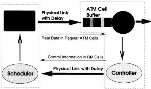
Physical Link with Delay

Scheduler

--- _;

:.! ii!•iiiiiiii? ii iiii•~ ~ ~iiiiii i i iii i

Real Data in Regular ATM Cells

Control Information in RM Cells

Physical Link with Delay

--- 4Bsf

---i,

ontroIer

Figure 1-1: General ATM Flow Control Model

quite sensitive to changes in some of these parameters. However, how to tune these parameters to attain optimal performance is far from being understood, because of the complexity involved and the nonlinear relationship between the dynamic performance and changes in the parameters.

ABR service specifies a rate-based feedback mechanism for flow control. The general idea of the mechanism is to adjust the input rates of sources on the basis of the current level of congestion along their VCs. It requires network switches to constantly monitor the traffic load and feed the information back to the sources. Unlike the flow control approach used in TCP, ATM-ABR can explicitly calculate the desired incoming rates and directly command these rates from the sources. Figure 1-1 presents a single node model of the flow control mechanism in an ATM network. Data encapsulated in ATM cells travels through the physical links . At the switch, the cells are buffered before they get serviced. The novelty in the ABR service is that the node also contains a controller which calculates a desired transmission rate for the sources. This rate information encapsulated in resource management (RM) cells is then sent back to the source

Recent interest in ABR service has brought about a vast amount of research activity on the design of feedback congestion control algorithms [1, 2, 8, 11, 12, 13,

a

ATIUI nill

(15)

---14, 17, 23, 24]. They differ from one another by the various switch mechanisms employed to determine the congestion information and the mechanisms by which the source rates are adjusted. Depending on the specific switch mechanisms employed, various congestion control algorithms yield different transient behaviors.

In [2], classical control theory is used to model the closed loop dynamics of a. congestion control algorithm. Using the analytical model, it addresses the problems of stability and fairness. However, as pointed out in [14], the algorithm is fairly complex and analytically intractable.

In [14], the congestion control problem is modeled by using only a first order system cascaded with a delay. The control algorithm is based on the idea, of the Smith predictor [25], which is used as a tool to overcome the possible instabilities caused by the delays in the network. The Smith predictor heavily relies on knowledge of the round-trip delay. The objective of this algorithm in is to minimize cell loss due to buffer overflow. However, the algorithm only uses the queue level in determining the rate command, and without knowledge of the service rate, there is always a steady-state error with respect to the desired queue level. When the service rate changes (as is often the case in ABR service), the algorithm may lead to underutilization of the link capacity. The major limitation of the algorithm is that it assumes that the network delay is known and remains constant. If the actual delay differs from the assumed constant delay, the controller response will exhibit oscillations and in some cases instability.

This thesis uses many of the ideas presented in [14]. The Smith predictor is seen as a tool to estimate the amount of data in the links. This measurement is the key to being able to design stable flow control algorithms. Likewise, the queue stabilization algorithm presented in [14] is one of the two key controller components presented in this thesis.

(16)

Data Source

)ata Source

Figure 1-2: Network Flow Control Model

1.3 Objective

This thesis focuses on network-based flow control schemes. In these schemes, the

network itself determines its level of congestion and determines how much data rate

it is willing to accept from the sources. We assume that the network can communicate this desired rate to sources and that the sources will comply. Under this framework (as seen in figure 1-2), the network is directly controlling the source behavior. This type of network-based flow control is more powerful than those based on the end users (i.e. TCP flow control) because the information relevant to solving the flow control problem is present inside the network.

This approach is directly applicable in ATM's ABR service since the ATM spec-ifications support this type of flow control. The switches can include their desired source rates in the explicit rate (ER) field contained in the RM cells returning to the source. The ATM source is then obliged to follow this explicit rate. At the same time, we would like to use the results in this thesis in an internetworking environ-ment where the sources are not directly connected to ATM. For this purpose, we take advantage of the fact that most data applications use TCP in their transport layer, regardless of the network technology they are traversing. The latter part of this thesis explains how a network node can control the transmission rate of a TCP source. This technique effectively extends our network-based flow control algorithms to any source

(17)

that uses TCP as its transport protocol.

1.4 Overview

Using a control theoretic framework, this thesis studies various ways in which an effective flow control policy can be obtained. Because of its direct applicability, the flow control schemes will be presented in the context of ATM.

Chapter 2 will introduce some of the basic tools and ideas that can be used to enforce a flow control policy. Basic terminology such as available rate and effective queue is explained and simple flow control mechanisms are presented. The last section of the chapter proves some of the fundamental limitations involved in controlling a network.

Chapter 3 describes the basic flow control model used in this thesis. The model combines the basic techniques from chapter 2. The model is analyzed and refined until we arrive at the central idea of this thesis: the separation principle.

Under this principle, the flow control mechanism is separated into two key com-ponents: rate reference control (RRC) and queue reference control (QRC). The RRC component determines its rate command by using measurements of the available bandwidth in each link, with the objective of adapting the input source rate to match the output available rate at steady state. On the other hand, the QRC component computes its rate command by using measurements of the queue level at each switch, with the goal of maintaining the queue level at a certain threshold. The desirable source rate is then equal to the sum of the QRC and RRC rate commands. The ad-vantage of this separation principle is that it decouples the complex dynamics of the closed-loop control system into two simpler control problems, which are analytically more tractable and can be solved independently.

Chapter 3 re-analyzes the separation principle from different viewpoints. The

QRC

component can be seen as an error observer of the RRC component. The

chapter also explains how the separation principle can be implemented using a primal as well as a dual structure. The primal structure relies on the RRC to maintain the

(18)

steady-state command, while the dual structure relies on the QRC for this task. In Chapter 4, various implementation issues are discussed. First, a discrete feed-back mechanism is developed which ensures stable and fast closed-loop dynamics. The available rate is defined in the multi-user context and an algorithm is derived to estimate this available rate. The separation principle is extended to the multi-node case. Finally, both the single-node and multi-node cases are simulated.

In Chapter 5, a specific flow control algorithm called bi-channel rate control (BRC) is presented. Apart from using the separation principle and the other techniques from the previous chapters, the BRC algorithm uses virtual data, and virtual queuing techniques. The virtual data technique creates a virtual channel in the network which is used for simulation purposes. This extra virtual channel allows the BRC algorithm to function without knowledge of the round-trip delay. The virtual queuing allows the algorithm to work in switches that use only FIFO queues. The new algorithm is simulated under the same conditions as the simulations in chapter 4.

Finally, in chapter 6 the TCP acknowledgment bucket scheme is presented. The idea behind this scheme is to manipulate the flow of TCP acknowledgments while they are traversing an ATM network so that the ATM network can control the rate of the TCP source. The scheme is implemented by using an acknowledgment bucket at the ATM network interface. Simulation results are also presented to demonstrate the effectiveness of the scheme.

(19)

Chapter 2 Basic Flow Control Ideas

In this chapter we will explore some of the basic ideas behind flow control algorithms. The purpose is to understand the fundamental difficulties one encounters as well as the various mechanisms that one can use in order to provide flow control. The first sections discuss various tools that can be used for the flow control problem. Using these tools, chapter 3 will expose a comprehensive model for our flow control system. In section 2.5, the fundamental time limitations of flow control are presented.

Our objective is to construct a controller that can regulate the flow of data enter-ing the network. We assume that the network has the computational capability to calculate the correct distribution of rates and communicate these desired rates to the sources. We also assume that the sources will comply with the rate commands.

In order to compute the rate command, the switches can use any information that is available to them, such as queue sizes, service rates per VC, and any information sent by the users or other switches. The switches can also estimate other states in the network, such as the amount of data in the links.

2.1 Using Service Rate

The simplest mechanism to control the flow of user data into the network is to com-mand the user to send data at a rate no greater than the service rate of the slowest switch in the virtual connection (VC). In steady state, the link is fully utilized and

(20)

there are no lost cells.

However, every time the service rate of the switch decreases, some cells can be lost. This inefficiency is due to the propagation delay in the links which prevents the source from reacting on time to changes in the service rates.

A major problem with this scheme is that the queue is unstable and cannot be controlled. In steady state, if there is any error in the service rate estimation, the queue will either always be empty or will grow until it overflows.

2.2 Using Queue Size

A slightly more complex flow control mechanism involves measuring the queue size at the switch. The switch computes a user data rate in order to fill the queue up to a reference queue size. This calculated rate is then sent as a command to the user. The computation of the rate requires a controller which outputs a rate command based on the error between the reference and real queue size. Since this control system attempts to stabilize the queue size to a certain level, it keeps the switch busy, maximizing throughput, while preventing cell loss.

However, as in the previous section, the propagation delays of the links prevent the source from reacting on time and can cause cell loss and unnecessary reduction of throughput. Furthermore, this system has the disadvantage that it can become unstable if the time delay or controller gain is sufficiently large.

2.3 Using Effective Queue Size

The instability of the preceding mechanism can be corrected by incorporating an effective queue into our controller. This effective queue includes all the data in the real queue of the switch, as well as the data that is traveling from the user to the switch and the data requests which are traveling from the switch to the source. The effective queue includes the number of cells that are bound to enter the real queue no matter what the switch commands in the future. Measurements or estimates of this

(21)

effective queue can be obtained using a Smith predictor or by using an accounting scheme. Both methods will be explained in the next section.

This control scheme is nearly identical to that in the previous section with the difference that the real queue size is replaced by the effective queue size. In this case, the controller tries to stabilize the effective queue size at a certain reference level. The advantage of this method is that since the switch can act on the effective queue instantaneously, there is no command delay and no instability due to such delay. In some sense, the system in which we are interested (queue) is modified so that it becomes easier to control.

The disadvantage of this technique is that the effective queue is not really what we are trying to control. When the data rate is smaller than the inverse of the link delay, the real queue is comparable to the effective queue and this approach is useful. However, as the data rate increases, the real queue becomes much smaller than the effective queue. At some point, in steady state, the real queue empties out and the data rate saturates. For high delay-bandwidth product connections, the data links are strongly under-utilized.

2.4 Estimating the Effective Queue Size

2.4.1 Accounting Estimator

One way of calculating the effective queue size is by using the accounting scheme. This is done by adding all the cells that the switch requests and subtracting all the cells that the switch receives. These cells that are "in flight" are then added to the real queue size, q(t). If u(t) is the rate command of the switch, a(t) is the arrival rate of cells at the switch, the estimate of the effective queue size q*(t) can be expressed

as:

(22)

This approach is similar to the credit based scheme. In fact, credits and q* are related by: credits = Maximum Queue Size - q*. The disadvantage of this method

is that it can be unstable. A disturbance in the number of cells that get sent would cause a permanent error in this estimate. For example, if a link is lossy and some percentage of the cells never make it to the queue, this estimator will add more cells than it subtracts, and the estimate will go to infinity.

2.4.2 Estimator with Smith Predictor

Another way of performing this calculation is by using a Smith predictor [25]. As in the previous method, the Smith predictor adds the number of cells that the switch requests and then subtracts them when they are expected to enter the switch's queue. This quantity is then added to the real queue's size. The calculation is done with the help of an artificial delay which figures out how many cells are about to enter the queue. If Test is the estimated round-trip delay, the estimate of the effective queue is:

E2[q*](t) = u(t)dt - u(T - Test)dT + q(t) (2.2)

The advantage of this second approach is that it is robust against disturbances: a constant error in u(t) will only produce a constant error in q*(t). The disadvantage is that a good a priori estimate of the round-trip time is needed. If this estimate is incorrect or the real round-trip time varies, this estimator might produce a large

error.

2.5 Transient Response and Performance

In this section, we will explore some of the fundamental limits on the transient re-sponse of flow control algorithms. We will show some of the restrictions that the network itself imposes on the controller.

(23)

inputs, and disturbances. The states of this system are the sizes of the various queues, the number of cells in the channels, and the control information traveling in the links. The inputs are the rates at which the sources are sending data. The disturbances are the switch service rates and the number of virtual channels passing through each switch. The purpose of a flow control algorithm is to compute the correct inputs to this system so as to stabilize its states in spite of the disturbances.

If all the disturbances of a communication network (i.e. the number of VCs and switch output rates) are stationary, it is easy to establish a flow control policy. The correct rate for each connection can be calculated off-line so as to prevent congestion and ensure a max-min fair allocation of bandwidth. This fair distribution will ensure that the network operates indefinitely in steady state.

If some of the disturbances of the network system change in a. completely

pre-dictable/ way, we can still calculate the correct allocations off-line and come up with

the fair source rates to enforce at each moment of time. In this ideal case, the network states stabilize to a new value immediately after the change in the disturbance.

If the disturbances change in an unpredictable manner, it will take some time for the flow control algorithm to stabilize the network. This settling time is the time required for the flow control algorithm to observe changes in the system and to control them. In other words, it is the time to reach steady-state operation after the last change in the disturbances. The settling time is mainly determined by the network delays.

2.5.1 Single Node Network

When the network contains only one node, we can obtain very strong bounds on the settling time. The settling time varies depending on whether the delay of the link between the source and the switch is known or not. The minimum bounds on the time needed to stabilize such systems are stated in the following theorems:

Theorem 1 For a network consisting of a single source and a single switch connected

(24)

can stabilize the network after a change in the switch's service rate is the round-trip

delay time (RTD) between the source and the switch.

Proof: Let us assume that at time zero the last change in the switch's service rate

takes place. Because the link delay is known, the controller can calculate the effects of this change on the network as soon as it knows of the change. Once the future effects are known, the controller can request the source to send data at a rate tha.t will correct the effects of the change of the service rate and immediately after at a rate that will reestablish steady-state operation. If the controller is located at the source, it will know of the service rate change at 1/2 RTD. If the controller is in the switch, it can send its new rate requests at time 0, but the requests will only reach the source at time 1/2 RTD. In both cases, the source starts sending data. at the new stable rate at time 1/2 RTD, which will only reach the switch at time 1 RTD. O

Note that this lower bound can only be achieved by a flow control algorithm that can accurately measure the disturbance (switch service rate), predict its effect on the network, and request new rates instantly that will reinstate the switch's queue size.

To prove the next theorem, we first need to prove the following lemma:

Lemma 1 For a network consisting of a single source and a single switch connected

by a link with an unknown delay, the minimum time needed to detect the effect of a change in the switch's service rate (given that the queue does not saturate) is the round-trip delay of the link (1 RTD).

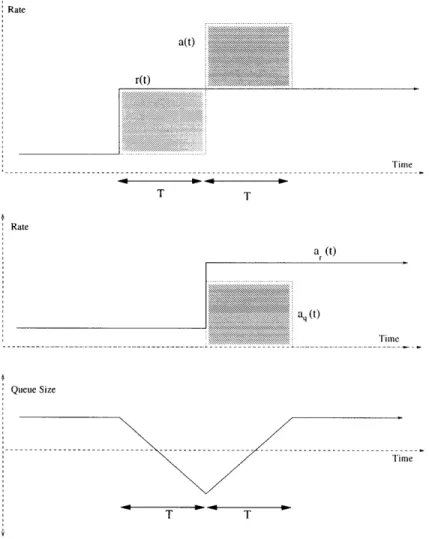
Proof: At the moment when the last change of the switch's service rate takes place

(time 0), the switch's output queue is changing (increasing or decreasing). Regard-less of what the controller does after time 0, the queue will continue to change in an uncontrollable manner for 1 RTD. This is the time that it takes for a new controller command to have an effect on the queue. Since the RTD is unknown, between time 0 and RTD, the controller does not know how much the queue size will change before its command has an effect on the queue. During this "unpredictable" period, the controller cannot know what the effect of the service rate change will be on the queue

(25)

RTD 2RTD

Steady State

RTD 2 RTD

Figure 2-1: Network with Unachievable Settling Time

size. It is only after time RTD that the controller can possibly know what the full consequence of the disturbance is on the queue size. The only exception is when the queue size saturates before time RTD; in this case, the controller knows the effect of

the rate change when the saturation occurs. E

Theorem 2 For a network consisting of a single source and a single switch connected

by a link with an unknown delay, the minimum time in which any flow control al-gorithm can stabilize the network after a change in the switch's service rate , given that the queue does not saturate, is twice the round-trip delay time (2 RTD) between the source and the switch.

Proof: Let us assume on the contrary that after the last change of the switch's

service rate at time 0, the network can be stabilized before time 2 RTD. Figure 2-1 shows an example of this scenario. In this case, the controller is located in the switch. Let u(t) be the instantaneous rate command given by the controller and a(t) be the arrival rate of data into the switch. Since we assumed that the system reaches steady state before 2 RTD, a(t) must reach steady state before 2 RTD (otherwise the queue size would oscillate). Because the source complies with the controller's command, we

(26)

know that a(t) = u(t-RTD). Therefore, u(t) must reach steady state before 1 RTD. This implies that the controller must know what the effect of the rate change at time

0 is before 1 RTD. From Lemma 1 we know that this is not possible if the queue does

not saturate. Therefore, our original assumption must be wrong, which proves the theorem. The same argument can be applied if the controller is located in the source

or any other place. O

Note that we have not proved that it is possible to stabilize the network in 2 RTD, but that it is impossible to do so in less than that time. From a. control-theoretic viewpoint, we can interpret this lower bound as the algorithm needing at least 1 RTD to observe the network and 1 RTD to control it.

2.5.2 Multiple Node Network

The transient response time in a multi-node network is much harder to analyze than in the single-node case. If some change of disturbance takes place in a particular node, it will trigger changes in the states of other nodes. These changes might propagate to the rest of the network.

The analysis is greatly simplified if we assume that there is no communication or collaboration between the different VCs in the network. From the perspective of one particular VC (which we will call VC i, the activities of the other VCs can be regarded as disturbances on the queue sizes and available bandwidth of VC i on each of its nodes. Furthermore, if the switches use a per-VC queuing discipline, the queue size of each VC will not be directly affected by the other VCs; the only disturbance apparent to VC i is the available bandwidth at each of its nodes.

We will assume that the VCs do not collaborate with each other. For the moment, we will also assume that the switches use a per-VC queuing discipline. Under these assumptions, we can determine the minimum time to achieve steady state in one particular node in a VC after a change in its available rate, given that the available rate at the other nodes in the VC are already in steady state. It is the time it takes for a control data unit that departs the node during the node's last change of

(27)

disturbance to travel to the source and back twice in a row. This is what we will refer to as "2 RTD" of a particular node in a, multi-node network. The time to complete the first loop is the minimum time needed to observe the effects of the last change of the disturbance on the VC, while the time to complete the second loop is the minimum time to control the VC queue at the node. This limit can be proved with the same arguments as in the proof of the single node case. The multi-node 2 RTD is determined by all the queuing delays upstream as well as by the propagation delays of the links.

Note that we have not shown anything about the global transient responses and stability of the entire network. We are just showing what is the shortest settling time possible for one VC if the other VCs are already in steady state.

(28)

Chapter 3 General Single Node Model and

Analysis

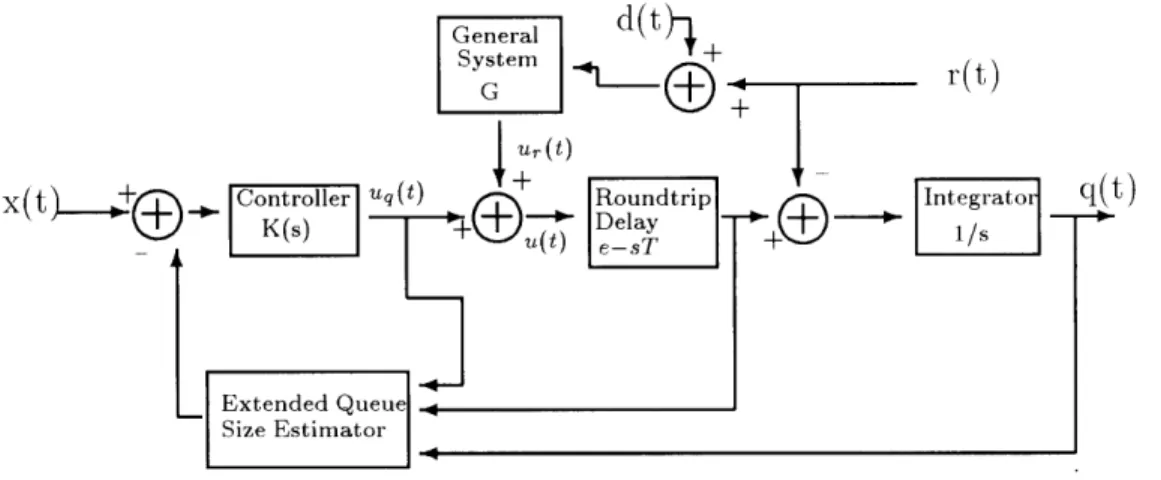
We will start our analysis by creating a general model which can use all the flow control schemes discussed in the previous chapter. The model is limited to the single node case. This model is a generalization of the one presented in [14]. The model uses a fluid approximation for all the data traffic and control signals.

On the left side of the model represented in figure 3-1, we can observe the control system that sends the rate command u(t) to the source. This command is sent to the source and returns as an actual data rate. The feedback and data channel are modeled as a delay e-ST where T is the round-trip delay time. The rate of incoming data is integrated to obtain the real queue size q(t). At the same time, the integral of the service rate r(t) is subtracted out of the queue size to reflect that the queue is being serviced.

The rate command u(t) is the sum of the commands u,(t) and uq(t), which are based on the service rate and effective queue size information respectively. We will refer to the subsystems with outputs u,(t) and u,(t) as queui reference control (QRC) and rate reference control (RRC) respectively.

The QRC contains an observer which estimates the effective queue size. This estimate is compared to the desired queue size x(t) and the error is fed into a controller

(29)

qC u)

X(t

+

_

Figure 3-1: General Model of Flow Control System

a system G (not necessarily linear) which takes as an input an approximation of the service rate rapp(t) and outputs the RRC part of the source rate u,.(t). The general model of rapp(t) is some disturbance d(t) added to the real service rate r(t).

This model allows us to use any combination of methods described in the last chapter. The main innovation in this model is that it allows for the combination of subsystems that can use both the service rate and the effective queue size as control information.

3.1 Primal Control Model

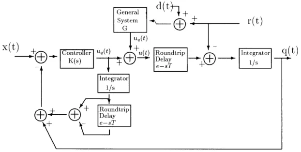
We have seen in the previous chapter that under ideal circumstances, the smith pre-dictor and the accounting system should have the same behavior in estimating the effective queue size. In isolated environments, QRC controllers that use a Smith pre-dictor or a an accounting system have identical dynamics (given that all parameters are correct). However when the RRC is added to the system, the overall system dy-namics are different for each case. For the moment, we will concentrate in describing the behavior of the system using a Smith predictor as shown in figure 3-2. We call call this model the primal control model. Later on, in section 3.3, we will show how to modify and reanalyze the system for when it uses an accounting system rather than a Smith predictor.

/L\

__P_

(30)

General

d(t

+

System _r(t)

/ \

XýT) ₄

Figure 3-2: Primal Control Model

3.1.1 Input/Output Relations

For the moment, let us also assume that the subsystem G is linear time-invariant (LTI). Now, the complete continuous time model is LTI. Its dynamics can be com-pletely characterized in terms of the transfer functions between its inputs and outputs. The relevant inputs are: x(t), r(t), and d(t). The only relevant output is q(t),the queue size.

The transfer functions between the inputs x(t), r(t), d(t) and the output q(t) are:

Q(s)

K(s)e-

T

₍

X(s)

s + K(s)

H(8)

Q(s)

G(s)e-sT -1 I + K(s) (1--e-sT) R(s) s + K (s) 3.2)

1 +

Q

-

1 e-1(

HI(s) s) -sT (33)

Hs

K(s)

G(s)e

(3.3)

With these transfer functions, we can completely determine q(t) from the inputs. In the following subsection we will describe the system's response to each of the inputs. Note that the total response is the superposition of the response to each input: q(t) = q,(t) + qr(t) + qd(t).

(31)

3.1.2 Response to Desired Queue Size

First of all, we would like qx(t) to follow x(t) as closely and as fast as possible. In steady state (if x(t) is a constant Xo), we would like qx(t) = x(t) = X0. In terms of the the transfer function shown in equation (3.1), this means that Hx(s) should be one for s = 0. A good response to a change in x(t) requires that Hf,(s) be close to one at least for small s.

A simple and efficient way of obtaining these results is to set K(s) to a constant

k. The simplified transfer function is:

H(s)= e T (3.4)

When k is large, q,(t) follows x(t) closely for low frequencies (small s). Further-more, the response is always a first order exponential followed by a delay. This means that there are no unwanted oscillations and the output is always stable (for this in-put). A larger k will offer a better response. However, we will later see that k is limited by the frequency of the feedback.

3.1.3 Response to the Service Rate

Now, we will examine how q,(t) varies with r(t). This knowledge is of particular importance because it tells us what type of service rate behavior will make the queue overflow or empty out. This calculation can be accomplished by convolving the im-pulse response of the system with r(t). For the moment, we assume that G is a constant g for all s. The queue's response q,(t) to an impulse in the switch rate r(t) simplifies to:

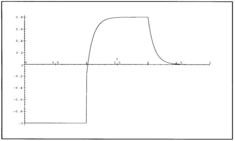
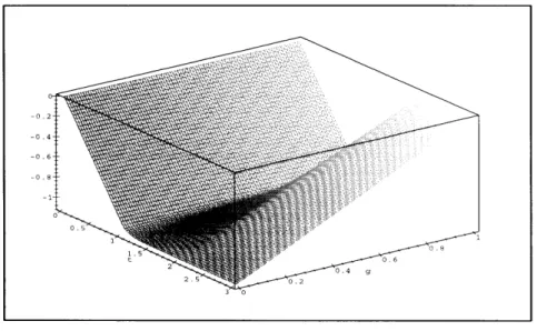
hr(t)

= -u(t) + + g - e-k(t-T)) u(t -- T) (g - ( -k(2T) g) u(t - 2T),

(32)

Figure 3-3: Impulse Response h,(t) with k=10, g=0.8, T=1 where u(t) is the unit step function.

This impulse response with a given set of parameters is illustrated in figure 3-3. For large enough gain k, this impulse response has the nice property of approximating two contiguous boxes with width T and heights -1 and g. Therefore, the queue size response caused by r(t) at any time t can be approximated by:

q,(t) g 2T r()d - Tr(r)d (3.6)

When the approximation is true, we only need information on r(t) from t - 2T to

t to obtain qr(t). If the service rate does not change much relative to the round-trip

time T, this calculation is easy to compute.

This approximation shows how instantaneous q(t) does not depend on on the instantaneous r(t), but rather on r(t) averaged over time intervals t - 2T to t - T

and t - T to t. This means that if r(t) oscillates wildly at very high frequencies, the

queue size will not be affected as long as the time averaged q(t) is reasonably stable. When g = 0, qr(t) is always negative, meaning that q(t) < q, ~ x (t). If x(t) is less

(33)

This is the scheme proposed in [14]. Its disadvantage is that in steady state there is a difference between the desired queue size x(t) and the actual queue size q(t). For high rates, the queue will empty out and the link will not be fully utilized.

If g = 1, qr(t) can be either positive or negative. The actual queue can either overflow or empty out. The advantage of this scheme is that in steady state (r(t) is constant), the queue level q(t) is always equal to the desired level x(t). In this case, the queue is stable and the link is fully utilized.

If 0 < g < 1, we can obtain a a queue behavior that is a weighted average of the two previous ones. If the delay-bandwidth product is low (r(t) x T << Max QueueM ,ize)

on average, we might set g to be closer to zero, since we are not losing much through-put and we can obtain a low cell loss performance. On the other hand, if the delay-bandwidth product is high on average, we might set g to be closer to one, since that will increase the throughput, even if the risk of losing cells is higher. Likewise, if we want cell loss to be minimized (i.e. for data transfer applications), we choose g small. If throughput is more important than occasional cell loss (i.e. for video transmissions), we choose a large g.

Step Response

In a real system, most of the changes in the service rate will be step changes. The service rate will be constant during certain intervals of time and will change abruptly when there is a change in the operation of the network, i.e. a new user connects, other services like VBR require bandwidth from ABR. By using Laplace transform methods, we can analytically determine how q,(t) will react to a unit step change in

1

--t)

qr(t) = -tu(t) + (I + g)(t - T)- 1 k(tT)- 1 (-T)

g(i1 - e-k(t-2T)

-

g(

-

2T) g(l

- (t-2T))u(t

-

2T)

.(3.7)

(34)

Figure 3-4: Step Response h,(t) for k=10,T=l

different values of g. Between time 0 and T, the system's new command has not traversed the delay yet, and q,(t) keeps moving away from its previous value. At time T, the system starts reacting with different strengths depending on the value of g. For g = 0, q,(t) stabilizes at T and does not recover from the change between 0 and T. For g = 1, q,(t) is restored at time 2T to its previous value, and the system stabilizes from there onwards. For 0 < g < 1, q,(t) only partially recovers its previous value. The response of a greater or smaller step is simply scaled appropriately.

Frequency Response

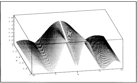
Another interesting characteristic of the system is the frequency response between

r(t) and qr(t). The frequency response describes how qr(t) reacts to sinusoidal inputs

of r(t) with different frequencies w and unit amplitude. In figure 3-5, we can see this frequency response with variable parameter g. A greater response for a particular w

means that qr(t) follows r(t) with a higher amplitude.

Ideally, we would like the frequency response to be zero for all w. This would mean that the queue does not react to the service rate. When g = 1 this is true for w = 0, which is equivalent to saying that there is no steady-state response. For smaller g, there appears some response at w = 0, and this response increases as g

(35)

Figure 3-5: Frequency Response IH,(s)l for k=10,T=1

gets smaller. However, when g is made smaller, the maximum frequency response (highest peak) decreases.

As mentioned earlier in this section, the response of the queue to oscillations of r(t) becomes negligible as the frequency of r(t) increases. The most perturbing frequencies are the ones comparable to the inverse of the delay time (w w r/T).

3.1.4 Error Sensitivity

We will finally analyze the system's sensitivity to an error d(t) in the measurement of the service rate. If an algorithm is purely RRC (k = 0), any finite d(t) can cause

qd(t) and the entire queue to be unstable (overflow or empty out). However, when

QRC is added to RRC, as in our model, qd(t) becomes stable.

From equations (3.2) and (3.3), we can see how the response to d(t) for any constant G(s) is proportional to the delayed part of the response to r(t). Both input/output relations are stable. This means that a finite d(t) will only cause a finite qd(t). Therefore, a finite error in the rate measurement will only cause a finite error in the real queue size.

(36)

3.2 Model Discussion and Improvements

3.2.1 Examining QRC and RRC Independently

Let us examine the dynamics between r(t) and q(t) when either K(s) is zero and

G(s) is one or G(s) is zero and K(s) is large. These two situations correspond to

using only the service rate (RRC) or the queue size (QRC) respectively as control references. From equation (3.5), we can see that the impulse response from r(t) to q(t) in each situation becomes:

-uC=

u(t -

r(t)

T)

(3.8)

h c ₌ _-u(t)_{_}

+

₍₁_- _{e-k(t-T))u(t -} _T)

-u(t) + u(t - T) . (3.9)

For large k, each type of control has the same response to changes in the service rate. In this case, the dynamics of QRC and RRC working independently are identical. Both algorithms are effective in utilizing the link bandwidth while the queue size is between its limits. However, both algorithms are ineffectual at stabilizing the queue size. In steady state as r(t) increases, q(t) decreases. As can be seen in figure 3-6, for a step change in r(t), the most each type of algorithm can do is to stop q(t) from changing after time T. Neither of them alone can recover from the change of q(t) between time 0 and T. From the same figure, we can see that the delay T in the response of RRC or QRC (with large k) to r(t) causes a change in the queue size

Aq(t) equal to the shaded area between the r(t) and u(t - T) curves.

The difference between the two independent controls arises when the system reaches the limits of the linearized model. The linearity of the model does not hold any longer once the queue is emptied out and more cells cannot be serviced , or when the queue overflows and more cells cannot enter the queue. In these cases, QRC behaves by freezing the rate command u(t), whereas RRC continues moving u(t) to-wards r(t). When the queue size is again within its limits and the linear regime is

(37)

SRate r(t) Time u(t-T) A q(t) Queue Size Time A q(t) T

Figure 3-6: Step Response of QRC or RRC as Isolated Systems

reestablished, QRC will be operating in the same region as before, while RRC will be operating in another region. In this case, the queue size resulting from RRC will have a constant offset from the corresponding command resulting from QRC. In general, a

QRC

algorithm will always generate the same queue size for the same constant service rate, while the RRC algorithm will generate a queue size that also depends on how many cells have been lost (full queue) or have not been utilized (empty queue).

Independent QRC and RRC each have a window of linear operation which limits the rate command it can issue when the system is in the linear regime. If the system is initialized with no service rate (r(t) = 0) and a constant queue reference (xr(t) = Xo), the initial window of operation is constrained by:

Xo - uma t Xo

min=

_T

< (T <

_T

(310)

where Qm,,x is the maximum queue size. When r(t) is beyond these limits, the system enters the non-linear regime. If r(t) < u,,in, cells are lost due to queue overflow, and

if r(t) > umax service slots are not being used. - - --- -- -- --

(38)

-In the case of QRC, its window is fixed, and u(t) always has the same constraints. On the other hand, for RRC, the linear operation window slides after delay T so that

r(t) will always be inside the window. The width of the window is constant (QWax/T),

but the edges will move to follow r(t) if it is operating in the non-linear regime. For QRC, if Xo < Qmax, r(t) can never be less than umi (since umin is negative). Therefore, the queue cannot overflow. In fact, the queue size of an independent QRC will always be less than X0. For this reason, independent QRC is a good control scheme for scenarios where we absolutely do not want cell loss. On the other hand, when r(t) > umax, QRC will be continuously missing service opportunities.

In RRC, the window of operation takes T time to follow r(t). During this delay, independent RRC will lose cells or miss service slots. However, after T, RRCQ will be back in the linear regime and fully utilize the link with no loss. For this reason, independent RRC is a good control choice when r(t) does not vary much and we want full utilization of the available links.

3.2.2 Superposition of QRC and RRC

Many of the problems and flaws of QRC and RRC can be corrected by making the two work together. In our original model this is equivalent to adding the output of

G(s) = 1 to the output of K(s) to obtain u(t). When this happens, the desired real

queue reference level is always attainable and throughput is always maximized. The two algorithms are complementary in nature, and one can correct the defects of the other.

In figure 3-7, we can observe the behavior of the cell arrival rate a(t) = u(t - T)

of the combined controller (with k large) after a step in r(t). For a time interval of T, the system does not react, and the queue size changes by an amount equal to the first shaded area. However, between time T and 2T, a(t) over-reacts by the right amount so that the previous queue level is restored by time 2T. Notice how the area of the second shaded region is the negative of that of the first region. After time 2T, a(t) is equal to q(t) and the queue size and the system in general are stable.

(39)

Rate Time Rate a (t) aq (t) Time Queue Size T T

Figure 3-7: Step Response of the Superposition of QRC and RRC

i

Design and analysis of flow control algorithms for data networks

Design and Analysis of Flow Control Algorithms

for Data Networks

by

Paolo L. Narvaez Guarnieri

S.B., Electrical Science and Engineering (1996)

Massachusetts Institute of Technology

Submitted to the Department of Electrical Engineering and Computer

Science

in partial fulfillment of the requirements for the degree of

Master of Engineering in Electrical Engineering and Computer Science

at the

MASSACHUSETTS INSTITUTE OF TECHNOLOGY

June 1997

@

Paolo L. Narvaez Guarnieri, MCMXCVII. All rights reserved.

The author hereby grants to MIT permission to reproduce and

distribute publicly paper and electronic copies of this thesis document

in whole or in part, and to grant others the right to do so.

i / n/

OCT 2 9

1997

Author ..

Department of Electrical Engineerin~

an

omputer Science

.,

May 9, 1997

k ai-Yeung (Sunny) Siu

tant Professor of Mechanical Engineering

Accepted by.

Arthur C. Smith

Chairman, Department Committee on Graduate Theses

Design and Analysis of Flow Control Algorithms for Data

Networks

by

Paolo L. Narviez Guarnieri

Abstract

Acknowledgments

Contents

List of Figures

C(s) ...

50

Chapter 1

Introduction

1.1

Flow Control

1.2

History

1.2.1

Transmission Control Protocol (TCP)

1.2.2

Asynchronous Transfer Mode (ATM)

Scheduler

ontroIer

1.3

Objective

1.4

Overview

QRC

Chapter 2

Basic Flow Control Ideas

2.1

Using Service Rate

2.2

Using Queue Size

2.3

Using Effective Queue Size

2.4

Estimating the Effective Queue Size

2.4.1

Accounting Estimator

2.4.2

Estimator with Smith Predictor

2.5

Transient Response and Performance

2.5.1

Single Node Network

2.5.2

Multiple Node Network

₍

_T

_T