Publisher’s version / Version de l'éditeur:
Survey of Text Mining II: Clustering, Classification, and Retrieval
READ THESE TERMS AND CONDITIONS CAREFULLY BEFORE USING THIS WEBSITE.
https://nrc-publications.canada.ca/eng/copyright
Vous avez des questions? Nous pouvons vous aider. Pour communiquer directement avec un auteur, consultez la première page de la revue dans laquelle son article a été publié afin de trouver ses coordonnées. Si vous n’arrivez pas à les repérer, communiquez avec nous à [email protected].
Questions? Contact the NRC Publications Archive team at
[email protected]. If you wish to email the authors directly, please see the first page of the publication for their contact information.
NRC Publications Archive
Archives des publications du CNRC
Access and use of this website and the material on it are subject to the Terms and Conditions set forth at
A Probabilistic Model for Fast and Confident Categorisation of Textual
Documents
Goutte, Cyril
https://publications-cnrc.canada.ca/fra/droits
L’accès à ce site Web et l’utilisation de son contenu sont assujettis aux conditions présentées dans le site LISEZ CES CONDITIONS ATTENTIVEMENT AVANT D’UTILISER CE SITE WEB.
NRC Publications Record / Notice d'Archives des publications de CNRC:
https://nrc-publications.canada.ca/eng/view/object/?id=05e3038a-f734-4b14-bcc4-d90f41df31e8 https://publications-cnrc.canada.ca/fra/voir/objet/?id=05e3038a-f734-4b14-bcc4-d90f41df31e8
A Probabilistic Model for Fast and
Confident*
Goutte, C.
2007
*Survey of Text Mining (edited by M. Berry et al.) 2007. NRC 49829.
Copyright 2007 by
National Research Council of Canada
Permission is granted to quote short excerpts and to reproduce figures and tables from this report, provided that the source of such material is fully acknowledged.
Categorisation of Textual Documents
Cyril Goutte
Interactive Language Technology
NRC Institute for Information Technology
283 Boulevard Alexandre Tach, Gatineau, QC J8X 3X7, Canada [email protected]
Summary. We describe the National Research Council’s entry in the Anomaly Detection/Text Mining competition organised at the Text Mining Workshop 2007. This entry relies on a straightforward implementation of a probabilistic categoriser described earlier [4]. This categoriser is adapted to handle multiple labelling and a piecewise-linear confidence estimation layer is added to provide an estimate of the labelling confidence. This technique achieves a score of 1.689 on the test data. This model has potentially useful features and extensions such as the use of a category-specific decision layer or the extraction of descriptive category keywords from the probabilistic profile.
1 Overview
This paper describes NRC’s entry to the Anomaly Detection/Text Mining competition organised at the Text Mining Workshop 2007.1
We relied on an implementation of a previously described probabilistic categoriser [4]. One of its desirable features is that the training phase is extremely fast, requiring only a single pass over the data to compute the summary statistics used to estimate the parameters of the model. Prediction requires the use of an iterative maximum likelihood technique (Expectation Maximisation, or EM, [1]) to compute the posterior probability that each document belongs to each category.
Another attractive feature of the model is that the probabilistic profiles as-sociated with each class may be used to describe the content of the categories. Indeed, even though, by definition, class labels are known in a categorisation task, those labels may not be descriptive. This was the case for the contest data, for which only category number were given. It is also the case for exam-ple with some patent classification systems (eg a patent on text categorization
1
may end up classified as “G06F 15/30” in the international patent classifica-tion, or “707/4” in the U.S.).
In the following section, we describe the probabilistic model, the training phase and the prediction phase. We also address the problem of providing multiple labels per documents, as opposed to assigning each document to a single category. We also discuss the issue of providing a confidence measure for the predictions and describe the additional layer we used to do that. Sec-tion 3 describes the experimental results obtained on the competiSec-tion data. We provide a brief overview of the data and we present results obtained both on the training data (estimating the generalisation error) and on the test data (the actual prediction error). We also explore the use of category-specific de-cisions, as opposed to on global decision layer, as used for the competition. We also show the keywords extracted for each category and compare those to the official class description provided after the contest.
2 The probabilistic model
Let us first formalise the text categorisation problem, such as proposed in the Anomaly Detection/Text Mining competition. We are provided with a set of M documents {di}i=1...M and associated labels ℓ ∈ {1, . . . C} where C is the
number of categories. These form the training set D = {(di, ℓi)}i=1...M. Note
that, for now, we will assume that there is only one label per document. We will address the multi-label situation later in section 2.3. The text categorisation task is the following: given a new document ed 6∈ D, find the most appropriate label eℓ. There are mainly two flavours of inference for solving this problem [15]. Inductive inference will estimate a model bf using the training data D, then assign ed to category bf ( ed). Transductive inference will estimate the label e
ℓ directly without estimating a general model.
We will see that our probabilistic model shares similarities with both. We estimate some model parameters, as described in section 2.1, but we do not use the model directly to provide the label of new documents. Rather, prediction is done by estimating the labelling probabilities by maximising the likelihood on the new document using an EM-type algorithm, cf. section 2.2.
Let us now assume that each document d is composed of a number of words w from a vocabulary V. We use the bag-of-word assumption. This means that the actual order of words is discarded and we only use the frequency n(w, d) of each word w in each document d. The categoriser presented in [4] is a model of the co-occurrences (w, d). The probability of a co-occurrence, P (w, d) is a mixture of C multinomial components, assuming one component per category:
P (w, d) =
C
X
c=1
= P (d)
C
X
c=1
P (c|d)P (w|c)
This is in fact the model used in Probabilistic Latent Semantic Analysis (PLSA, cf. [8]), but used in a supervised learning setting. The key modelling aspect is that documents and words are conditionally independent, which means that within each component, all documents use the same vocabulary in the same way. Parameters P (w|c) are the profiles of each category (over the vocabulary), and parameters P (c|d) are the profiles of each document (over the categories). We will now show how these parameters are estimated from the training data.
2.1 Training
The (log-)likelihood of the model with parameters θ = {P (d); P (c|d); P (w|c)} is: L(θ) = log P (D|θ) =X d X w∈V n(w, d) log P (w, d), (2)
assuming independently identically distributed (iid) data.
Parameter estimation is carried out by maximising the likelihood. Assum-ing that there is a one-to-one mappAssum-ing between categories and components in the model, we have, for each training document, P (c = ℓi|di) = 1 and
P (c 6= ℓi|di) = 0, for all i. This greatly simplifies the likelihood, which may
now be maximised analytically. Let us introduce |d| =Pwn(w, d) the length of document d, |c| =Pd∈c|d| the total size of category c (using the shorthand notation d ∈ c to mean all documents disuch that ℓi= c), and N =Pd|d| the
number of words in the collection. The Maximum Likelihood (ML) estimates are: b P (w|c) = 1 |c| X d∈c n(w, d) and P (d) =b |d| N (3)
Note that in fact only the category profiles bP (w|c) matter. As shown below, the document probability bP (d) is not used for categorising new documents (as it is irrelevant, for a given d).
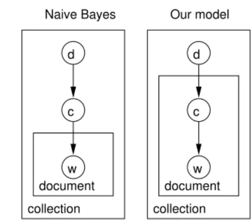
The ML estimates in eq. 3 are essentially identical to those of the Na¨ıve Bayes categoriser [12]. The underlying probabilistic models, however, are def-initely different, as illustrated on figure 1 and shown in the next section. One key consequence is that the probabilistic model in eq. 1 is much less sensitive to smoothing than Na¨ıve Bayes.
It should be noted that the ML estimates rely on simple corpus statistics and can be computed in a single pass over the training data. This contrasts with many training algorithm that rely on iterative optimisation methods. It means that training our model is extremely computationally efficient.
d c w document document w c d Our model Naive Bayes collection collection
Fig. 1.Graphical models for Na¨ıve Bayes(left) and for the probabilistic model used here (right).
2.2 Prediction
Note that eq. 1 is a generative model of co-occurrences of words and docu-ments within a given collection {d1. . . dn} with a set vocabulary V. It is not
a generative model of new documents, contrary to, for example, Na¨ıve Bayes. This means that we can not directly calculate the posterior probability P ( ed|c) for a new document.
We obtain predictions by folding in the new document in the collection. As document ed is folded in, the following parameters are added to the model: P ( ed) and P (c| ed), ∀c. The latter are precisely the probabilities we are interested in for predicting the category labels. As before, we use a Maximum Likelihood approach, maximising the likelihood for the new document:
e L =X w n(w, ed) log P ( ed)X c P (c| ed)P (w|c) (4)
with respect to the unknown parameters P (c| ed).
The likelihood may be maximised using a variant of the Expectation Max-imisation (EM, cf. [1]) algorithm. It is similar to the EM used for estimating the PLSA model (see [8, 4]), with the constraint that the category profiles P (w|c) are kept fixed. The iterative update is given by:
P (c| ed) ← P (c| ed)X w n(w, ed) | ed| P (w|c) P cP (c| ed)P (w|c) (5) The likelihood (4) is guaranteed to be strictly increasing with every EM step, therefore equation 5 converges to a (local) minimum. In the general case of unsupervised learning, the use of deterministic annealing [14] during pa-rameter estimation helps reduce sensitivity to initial conditions and improves convergence (cf. [8, 4]). Note however that as we only need to optimise over
a small set of parameters, such annealing schemes are typically not necessary at the prediction stage. Upon convergence, the posterior probability estimate for P (c| ed) may be used as a basis for assigning the final category label(s) to document ed.
Readers familiar with Non-negative Matrix Factorization (NMF, cf. [10]) will have noticed that eq. 5 is very similar to one of the update rules used for estimating the NMF that minimises a KL-type divergence between the data and the model. Indeed, the unsupervised counterpart to our model, PLSA, is essentially equivalent to NMF in this context [3]. Therefore, another way of looking at the categorisation model described in this paper is in fact to view it as a constrained NMF problem, with the category labels providing the constraint on one of the factors (the loading).
The way the prediction is obtained also sheds some light on the difference between our method and a Na¨ıve Bayes categoriser. In Na¨ıve Bayes, a cate-gory is associated with a whole document, and all words from this document must then be generated from this category. The occurrence of a word with a low probability in the category profile will therefore impose an overwhelm-ing penalty to the category posterior P (c|d). By contrast, the model we use here assigns a category c to each co-occurrence (w, d), which means that each word may be sampled from a different category profile. This difference mani-fests itself in the re-estimation formula for P (c| ed), eq. 5, which combines the various word probabilities as a sum. As a consequence, a very low probabil-ity word will have little influence on the posterior category probabilprobabil-ity and, more importantly, will not impose an overwhelming penalty. This key differ-ence also makes our model much less sensitive to probability smoothing than Na¨ıve Bayes. This means that we do not need to set extra parameters for the smoothing process. In fact, up to that point, we do not need to set any extra hyper-parameter in either the training or the prediction phases.
As an aside, it is interesting to relate our method to the two paradigms of inductive and transductive learning [15]. The training phase seems typically inductive: we optimise a cost function (the likelihood) to obtain one optimal model. Note however that this is mostly a model of the training data, and it does not provide direct labelling for any document outside the training set. At the prediction stage, we perform another optimisation, this time over the labelling of the test document. This is in fact quite similar to transductive learning. As such, it appears that our probabilistic model shares similarities with both learning paradigms.
We will now address two important issues of the Anomaly Detection/Text Mining competition that require some extensions to the basic model that we have presented. Multi-label categorisation is addressed in section 2.3 and the estimation of a prediction confidence is covered in section 2.4.
2.3 Multi-class,
So far, the model we have presented is strictly a multi-class, single-label cate-gorisation model. It can handle more than 2 classes (C > 2) but the random variable c indexing the categories takes a single value in a discrete set of C possible categories.
The Anomaly Detection/Text Mining competition is a class, multi-label categorisation problem: each document may belong to multiple cate-gories. In fact, although most documents have only one or two labels, one document, number 4898, has 10 labels (out of 22), and 5 documents have exactly 9 labels.
One principled way to extend our model to handle multiple labels per document is to consider all observed combinations of categories and use these combinations as single “labels”, as described eg in [11]. On the competition data, however, there are 1151 different label combinations with at least one as-sociated document. This makes this approach hardly practical. An additional issue is that considering label combinations independently, one may miss some dependencies between single categories. That is, one can expect that combina-tions (C4, C5, C10) and (C4, C5, C11) may be somewhat dependent as they share two out of three category labels. This is not modelled by the basic “all model combinations” approach. Although dependencies may be introduced as described for example in [7], this adds another layer of complexity to the system. In our case, the number of dependencies to consider between the 1151 observed label combinations is overwhelming.
Another approach is to reduce the multiple labelling problem to a number of binary categorisation problems. With 22 possible labels, we would therefore train 22 binary categorisers and use them to take 22 independent labelling decisions. This is an appealing and usually successful approach, especially with powerful binary categorisers such as Support Vector Machines [9]. However, it still mostly ignores dependencies between the individual labels (for example the fact that labels C4 and C5 are often observed together) and it multiplies the training effort by the number of labels (22 in our case).
Our approach is actually somewhat less principled than the alternatives mentioned above, but a lot more straightforward. We rely on a simple thresh-old a ∈ [0; 1] and assign any new document ed to all categories c such that P (c| ed) ≥ a. In addition, as all documents in the training set have at least one label, we make sure that ed always gets assigned the label with the high-est P (c| ed), even if this maximum is below the threshold. This threshold is combined with the calculation of the confidence level as explained in the next section.
2.4 Confidence estimation
A second important issue in the Anomaly Detection/Text Mining competition is that labelling has to be provided with an associated confidence level.
The task of estimating the proper probability of correctness for the output of a categoriser is sometimes called calibration [16]. The confidence level is then the probability that a given labelling will indeed be correct, ie labels with a confidence of 0.8 will be correct 80% of the time. Unfortunately, there does not seem to be any guarantee that the cost function used for the competition will be optimised by a “well calibrated” confidence (cf. section 3.2 below). In fact there is always a natural tension between calibration and performance. Some perfectly calibrated categorisers can show poor performance; Conversely, some excellent categorisers (for example Support Vector Machines) may be poorly or not calibrated.
Accordingly, instead of seeking to calibrate the categoriser, we use the provided score function, Checker.jar, to optimise a function that outputs the confidence level, given the probability output by the categoriser. In fields like speech recognition, and more generally in Natural Language Processing, confidence estimation is often done by adding an additional Machine Learning layer to the model [5, 2], using the output of the model and possibly additional, external features measuring the level of difficulty of the task. We adopt a similar approach, but using a much simpler model.
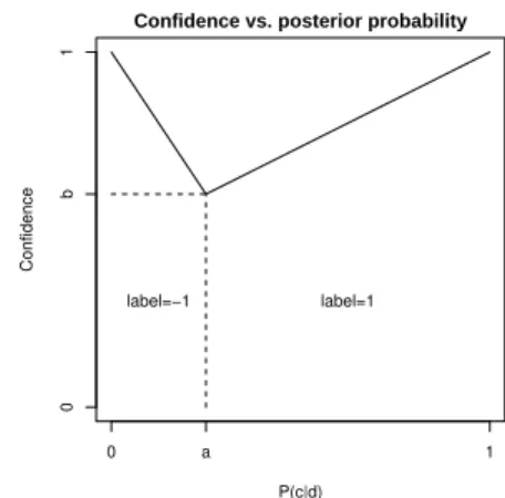
The confidence layer transforms the conditional probability output by the model, P (c| ed), into a proper confidence measure by using a piecewise linear function with two parameters (figure 2). One parameter is the probability threshold a, which determines whether a label is assigned or not; the second is a baseline confidence level b, which determines what confidence we give a document that is around the threshold. The motivation for the piecewise-linear shape is that it seems reasonable that the confidence is a monotonic function of the probability, ie if two documents ed1 and ed2 are such that a <
P (c| ed1) < P (c| ed2), then it makes sense to give ed2a higher confidence to have
label c than ed1. Using linear segments is a parsimonious way to implement
this assumption.
Let us note that the entire model, including the confidence layer, relies on only two learning parameters, a and b. These parameters may be optimised by maximising the score obtained on a prediction set or a cross-validation estimator, as explained below.
2.5 Category description
The model relies on probabilistic profiles P (w|c) which represent the proba-bility of each word of the vocabulary to be observed in documents of category c. These profiles allow us to identify which words are more typical of each category, and therefore may provide a way to interpret the data by providing descriptive keywords for each category.
Notice that the simplest way of doing this, by focusing on words w with the highest probabilities P (w|c), is not very efficient. First of all, the probability profile is linked to the frequency of words in the training corpus (eq. 3), and high frequency words tend to be grammatical (“empty”) words with no
Confidence vs. posterior probability P(c|d) Confidence 0 a 1 0 b 1 label=1 label=−1
Fig. 2. The piecewise linear function used to transform the posterior probability into a confidence level.
descriptive content. Even when grammatical words have been filtered out, words typical of the general topic of the collection (eg related to planes and aviation in the contest corpus, see below) will tend to have high frequency in many categories.
In order to identify words that are typical of a class c, we need to identify words that are relatively more frequent in c than in the rest of the categories. One way of doing that is to contrast the profile of the category P (w|c) and the “profile” for the rest of the data, i.e. P (w|¬c) ∝Pγ6=cP (w|γ). We express the difference between the two distributions by the symmetrised Kullback-Leibler divergence: KL(c, ¬c) =X w (P (w|c) − P (w|¬c)) log P (w|c) P (w|¬c) | {z } kw (6)
Notice that the divergence is an additive sum of word-specific contributions kw. Words with a large value of kw contribute the most to the overall
diver-gence, and hence to the difference between category c and the rest. As a con-sequence, we propose as keywords the words w for which P (w|c) > P (w|¬c) and kw is the largest.
2
In the following section, we will see how this strategy allows to extract keywords that are related to the actual description of the categories.
3 Experimental results
We will now describe some of our experiments in more details and give some results obtained both for the estimated prediction performance, using only
2
the training data provided for the competition, and on the test set using the labels provided after the competition.
3.1 Data
The available training data consists of 21519 reports categorised in up to 22 categories. Some limited pre-processing was performed by the organisers, eg tokenisation, stemming, acronym expansion and removal of places and num-bers. This pre-processing makes it non-trivial for participants to leverage their own in-house linguistic pre-processing. On the other hand, it places contes-tants on a level-playing field, which puts the emphasis on differences in the actual categorisation method, as opposed to differences in pre-processing.3
The only additional pre-processing we performed on the data was stop-word removal, using a list of 319 common stop-words. Similar lists are available many places on the Internet. After stop-word removal, documents were in-dexed in a bag-of-word format by recording the frequency of each word in each document.
In order to obtain an estimator of the prediction error, we organised the data in a 10-fold cross-validation manner. We randomly re-ordered the data and formed 10 splits: 9 containing 2152 documents, and one with 2151 docu-ment. We then trained a categoriser using each subset of 9 splits as training material, as described in section 2.1, and produced predictions on the remain-ing split, as described in 2.2. As a result, we obtain 21519 predictions on which we optimised parameters a and b.
Note that the 7077 test data on which we obtained the final results reported below were never used during the estimation of either model parameters or additional decision parameters (thresholds and confidence levels).
3.2 Results
The competition was judged using a specific cost function combining pre-diction performance and confidence reliability. For each category c, we com-pute the area under the ROC curve, Ac, for the categoriser. Ac lies between
0 and 1, and is usually above 0.5. In addition, for each category c, denote tic∈ {−1, +1} the target label for document di, yic∈ {−1, +1} the predicted
label and qic∈ [0; 1] the associated confidence. The final cost function is:
Q = 1 C C X c=1 (2Ac− 1) + 1 M M X i=1 qicticyic (7)
Given predicted labels and associated confidence, the reference script Checker.jar provided by the organisers computes this final score. A perfect
3
In our experience, differences in pre-processing typically yield larger performance gaps than differences in categorisation method.
prediction with 100% confidence yields a final score of 2, while a random assignment would give a final score around 0.
Using the script Checker.jar, on the cross-validated predictions, we opti-mised a and b using alternating optimisations along both parameters. The optimal values used for our submission to the competition are a = 0.24 and b = 0.93, indicating that documents are labelled with all categories that have a posterior probability higher than 0.24, and the minimum confidence is 0.93. This seems like an unusually high baseline confidence (ie we label with at least 93% confidence). However, this is not surprising if one considers the expression of the cost function (eq. 7) more closely. The first part is the area under the curve: this depends only on the ordering. Although the ordering is based on the confidence levels, it only depends on the relative, not the absolute, values. For example, with our confidence layer, the ordering is preserved regardless of the value of b, up to numerical precision.
On the other hand, the second part of the cost function (7) directly in-volves the confidence estimates qic. The value of this part will increase if we
can reliably assign high confidence (qic ≈ 1) to correctly labelled documents
(tic = yic) and low confidence (qic ≈ 0) to incorrectly labelled documents
(tic 6= yic). However, if we could reliably detect such situations, we would
arguably be better off swapping the label rather than downplay its influence by assigning it low confidence. So assuming we can not reliably do so, ie qic
and ticyicare independent, the second part of the cost becomes approximately
equal to q(2×M CE −1), with q the average confidence and M CE the misclas-sification error, M CE = 1/MPi(tic 6= yic). So the optimal strategy under
this assumption is to make q as high as possible by setting qic as close to 1
as possible, while keeping the ordering intact. This explains why a relatively high value of b turned out to be optimal. In fact, using a higher precision in our confidence levels, setting b to 0.99 or higher yields even better results.4
Using the setting a = 0.24 and b = 0.93, the cross-validated cost is about 1.691. With the same settings, the final cost on the 7,077 test documents is 1.689, showing an excellent agreement with the cross-validation estimate. In order to illustrate the sensitivity of the performance to the setting of the two hyper-parameters a and b, we plot the final cost obtained for various combinations of a and b, as shown in figure 3. The optimal setting (cross) is in fact quite close to the cross-validation estimate (circle). In addition, it seems that the performance of the system is not very sensitive to the precise values of a and b. Over the range plotted in figure 3, the maximal score (cross) is 1.6894, less than 0.05% above the CV-optimised value, and the lowest score (bottom left) is 1.645, 2.5% below. This means that any setting of a and b in that range would have been within 2.5% of the optimum.
4
Note however that setting b to higher value only yields marginal benefits in terms of final cost.
a b 0.1 0.2 0.3 0.4 0.6 0.7 0.8 0.9 Max. score CV
Fig. 3. Score for various combinations of a and b. The best (maximum) test score is indicated as a cross, the optimum estimated by cross-validation (CV) is a = 0.24 and b = 0.93, indicated by a circle.
We also measured the performance using some more common and intuitive metrics. For example, the overall mislabelling error rate is 7.22%, and the micro-averaged F -score is a relatively modest 50.05%.
Note however that we have used a single confidence layer, and in par-ticular a single labelling threshold a, for all categories. Closer inspection of the performance on each category shows quite a disparity in performance, and in particular in precision and recall, across the categories.5
This suggests that the common value of the threshold a may be too high for some cate-gories (hence low recall) and too low for others (hence low precision). Using the cross-validated prediction, we therefore optimised some category-specific thresholds using various metrics:
• Maximum F -score
• Break-even point (ie point at which precision equals recall) • Minimum error rate
For example, for maximum F -score, we optimised 22 thresholds, one per cat-egory, by maximising the F -score for each category on the cross-validated predictions.
Table 1 shows the performance obtained on the test data for all 22 cate-gories, using category-specific, maximum F -score optimised thresholds. Per-formance is expressed in terms of the standard metrics of precision, recall and F-score. The performance varies a lot depending on the category. However there does not seem to be any systematic relation between the performance
5
Precision estimates the probability that a label provided by the model is correct, while recall estimates the probability that a reference label is indeed returned by the model [6]. F-score is the harmonic average of precision and recall.
Category #docs p (%) r (%) F (%) C1 435 64.99 83.22 72.98 C2 3297 46.72 99.57 63.60 C3 222 74.06 79.73 76.79 C4 182 52.15 59.89 55.75 C5 853 80.07 75.38 77.66 C6 1598 51.33 80.98 62.83 C7 546 36.38 77.29 49.47 C8 631 55.32 67.51 60.81 C9 168 59.30 60.71 60.00 C10 349 37.21 58.74 45.56 C11 161 77.44 63.98 70.06 Category #docs p (%) r (%) F (%) C12 918 72.02 79.08 75.39 C13 687 51.21 55.46 53.25 C14 393 68.73 70.48 69.60 C15 183 30.61 24.59 27.27 C16 314 32.93 60.83 42.73 C17 162 45.22 43.83 44.51 C18 351 57.30 58.12 57.71 C19 1767 61.54 80.42 69.73 C20 229 72.40 69.87 71.11 C21 137 78.79 56.93 66.10 C22 233 88.66 73.81 80.56 Table 1. Performance of the probabilistic model: precision, recall and F -score for each of the 22 categories. Low (< 50%) scores are in italics and high (> 75%) scores are in bold. Column “# docs” contains the number of test documents with the corresponding label.
and the size of the categories. The worst, but also the best performance are observed on small categories (less that 250 positive test documents). This suggests that the variation in performance may be simply due to varying in-trinsic difficulty of modelling the categories. The best F-scores are observed on categories C3, C5, C12 and C22, while categories C15, C16, C17, C10 and C7 get sub-50% performance.
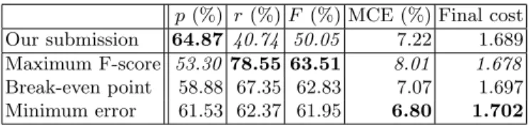
The average performance is presented in table 2 for our submission to the competition, as well as for three different strategies for optimising a category-per-category threshold. One weakness of the original submission was the low recall, due to the fact that a single threshold was used for all 22 categories. This produces a relatively low average F -score of 50.05%. By optimising the threshold for each category over various performance measures, we largely improve over that. Not surprisingly, optimising the thresholds for F -scores yields the best test score of 63.51%, although both the misclassification error and the final cost degrade using this strategy. Optimising the threshold for reducing the misclassification error reduces the test misclassification error6
to 6.80% and improves the final cost slightly, to 1.702. Notice however that, despite a large impact on F -score and MCE, using category-specific decision thresholds optimised over various thresholds seems to have little impact on the final cost, which stays within about 0.8% of the score of our submission. 3.3 Category description
The only information provided by the organisers at the time of the contest was the labelling for each document, as a number between 1 and 22. This data
6
For 7077 test documents with 22 possible labels, reducing the MCE by 0.1% corresponds to correcting 156 labelling decisions.
p(%) r (%) F (%) MCE (%) Final cost Our submission 64.87 40.74 50.05 7.22 1.689 Maximum F-score 53.30 78.55 63.51 8.01 1.678 Break-even point 58.88 67.35 62.83 7.07 1.697 Minimum error 61.53 62.37 61.95 6.80 1.702
Table 2.Micro-averaged performance for our contest submission, and three thresh-old optimisation strategy. Highest is best for precision(p), recall (r), F -score (F ) and final cost (eq. 7), and lowest is best for misclassification error (MCE).
therefore seemed like a good test bed for applying the category description technique described above, and see whether the extracted keywords brought any information on the content of the categories.
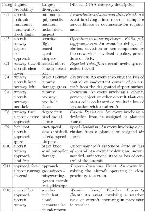
Table 3 shows the results we obtained on about half the categories by extracting the top 5 keywords. For comparison, we also extracted the 5 words with highest probability (first column), and we also give the official category description from the Distributed National Aviation Safety Action Program Archive (DNAA), which were released after the competition.
Based on only 5 keywords, the relevance of the keywords provided by ei-ther highest probability or largest divergence and their mapping to the official category descriptions are certainly open to interpretation. The most obvious problem with the choice of the highest probability words, however, is that the same handful of keywords seem to appear in almost all categories. The words “aircraft” is among the top-5 probability in 19 out of 22 categories! Although it is obviously a very relevant and common word for describing issues dealing with aviation, it is clearly not very useful to discriminate the content of one category versus the others. The other frequent members of the top-5 highest probability are: runway (14 times), airport (11), approach (11), feet (9) and land (9). These tend to “pollute” the keyword extraction: for example in cat-egory C8 (Course deviation), 3 out of the 5 highest probability keywords are among these frequent keywords and bring no relevant descriptive information. The remaining 2 keywords, “turn” and “degree”, on the other hand seem like reasonable keywords to describe course deviation problems. By contrast, the five words contributing to the largest divergence, “degree”, “turn”, “head”, “radial” and “course” appear as keywords only for this category, and they all seem topically related to the corresponding problem. For the largest diver-gence metric, kw, the word selected most often in the top-5 is “runway”, which
describes 6 categories containing problems related to take-off or landing (eg C3, C4, C5 and C6). Other top-5 keywords appear in at most 4 categories. This suggests that using kw instead of P (w|c) yields more diverse and more
descriptive keywords.
This is also supported by the fact that only 32 distinct words are used in the top-5 highest probability keywords over the 22 categories, while the top-5 largest kw selects 83 distinct words over the 22 categories. This further
reinforces the fact that kw will select more specific keywords, and discard the
words that are common to all categories in the corpus.
This is well illustrated on category C13 (Weather Issue). The top-5 prob-ability words are all among the high probprob-ability words mentioned above. By contrast, the top-5 kw are all clearly related to the content of category C13,
such as “weather”, “cloud”, “ice” or “thunderstorm”.
Overall, we think that this example illustrates the shortcomings of the choice of the highest probability words to describe a category. It supports our proposition to use instead words that contribute most to the divergence be-tween one categroy and the rest. These provide a larger array of keywords and seem more closely related to the specificities of the categories they describe.
4 Summary
We have presented the probabilistic model that we used in NRC’s submission to the Anomaly Detection/Text Mining competition at the Text Mining Work-shop 2007. This probabilistic model may be estimated from pre-processed, indexed and labelled documents with no additional learning parameters, and in a single pass over the data. This makes it extremely fast to train. On the competition data, in particular, the training phase takes only a few seconds on a current laptop. Obtaining predictions for new test documents requires a bit more calculations but is still quite fast. One particularly attractive feature of this model is that the probabilistic category profiles can be used to provide descriptive keywords for the categories. This is useful in the common situation where labels are known only as codes and the actual content of the categories may not be known to the practitioner.
The only training parameters we used are required for tuning the decision layer, which selects the multiple labels associated to each documents, and estimates the confidence in the labelling. In the method that we implemented for the competition, these parameters are the labelling threshold, and the confidence baseline. They are estimated by maximising the cross-validated cost function.
Performance on the test set yields a final score of 1.689, which is very close to the cross-validation estimate. This suggests that despite its apparent simplicity, the probabilistic model provides a very efficient categorisation. This is actually corroborated by extensive evidence on multiple real-life use cases. The simplicity of the implemented method, and in particular the some-what rudimentary confidence layer, suggests that there may be ample room for improving the performance. One obvious issue is that the ad-hoc layer used for labelling and estimating the confidence may be greatly improved by using a more principled approach. One possibility would be to train multiple categorisers, both binary and multi-category, and use the output of these cat-egorisers as input to a more complex model combining this information into a proper decision associated with a better confidence level. This may be done for
Categ Highest probability
Largest divergence
Official DNAA category description C1 aircraft maintain minimume-quipmentlist check flight minimume-quipmentlist maintain install defer inspect Airworthiness/Documentation Event: An event involving a incorrect or incomplete airworthiness or documentation require-ment C2 aircraft runway airport feet approach security flight board agent airspace
Operation in noncompliance - FARs, pol-icy/procedures: An event involving a vi-olation, deviation or non-compliance by the crew which involved a policy, proce-dure or FAR. C3 runway takeoff aircraft clear tower takeoff abort runway reject roll
Rejected Takeoff: An event involving a re-jected takeoff C4 runway aircraft land taxiway left brake taxiway runway damage grass
Excursion: An event involving the loss of control or inadvertent control of an air-craft from the designated airport surface C5 runway aircraft taxiway taxi hold runway taxiway taxi hold short
Incursion: An event involving a vehicle, person, object or other aircraft that cre-ates a collision hazard or results in loss of separation with an aircraft
C8 runway turn airport degree approach degree turn head radial course
Course Deviation: An event involving a deviation from an assigned or planned course C9 feet knot aircraft approach speed knot speed slow knotsindi-catedairspeed airspeed
Speed Deviation: An event involving a de-viation from a planned or assigned air speed C10 aircraft runway approach land feet brake knot wind autopilot damage
Uncommanded/Unintended State or loss of control: An event involving an uncom-manded, unintended state or loss of con-trol of the aircraft
C11 approach feet airport runway descend approach groundproxi- mitywarning-system terrain feet glideslope
Terrain Proximity Event: An event in-volving the aircraft operating in close proximity to terrain. C13 airport feet approach aircraft runway weather turbulent cloud encounter ice thunderstorm
Weather Issue/ Weather Proximity Event: An event involving a weather issue or aircraft operating in proximity to weather.
Table 3.Keywords extracted for 12 of the contest categories using either the highest probability words or the largest contributions to the KL divergence. For comparison, the official description from the DNAA, released after the competition, is provided.
example using a simple logistic regression. Note that one issue here is that the final score used for the competition, eq. 7, combines a performance-oriented measure (area under the ROC curve) and a confidence-oriented measure. As a consequence, and as discussed above, there is no guarantee that a well-calibrated classifier will in fact optimise this score. Also, this suggests that there may be a way to invoke multi-objective optimisation in order to further improve the performance.
Among other interesting topics, let us mention the sensitivity of the method to various experimental conditions. In particular, although we have argued that our probabilistic model is not very sensitive to smoothing, it may very well be that a properly chosen smoothing, or similarly, a smart feature selection process, may further improve the performance. In the context of multi-label categorisation, let us also mention the possibility to exploit de-pendencies between the classes, for example using an extension of the method described in [13].
References
1. A. P. Dempster, N. M. Laird, and D. B. Rubin. Maximum likelihood from incomplete data via the EM algorithm. Journal of the Royal Statistical Society, Series B, 39(1):1–38, 1977.
2. Simona Gandrabur, George Foster, and Guy Lapalme. Confidence estimation for NLP applications. ACM Transactions on Speech and Language Processing,, 3(3):1–29, 2006.
3. Eric Gaussier and Cyril Goutte. Relation between PLSA and NMF and implica-tions. In Proceedings of the 28th Annual International ACM SIGIR Conference, pages 601–602, 2005.
4. Eric Gaussier, Cyril Goutte, Kris Popat, and Francine Chen. A hierarchical model for clustering and categorising documents. In Advances in Information Retrieval, Lecture Notes in Computer Science, pages 229–247. Springer, 2002. 5. L. Gillick, Y. Ito, and J. Young. A probabilistic approach to confidence
estima-tion and evaluaestima-tion. In ICASSP ’97: Proceedings of the 1997 IEEE Internaestima-tional Conference on Acoustics, Speech, and Signal Processing, volume 2, pages 879– 882, 1997.
6. Cyril Goutte and Eric Gaussier. A probabilistic interpretation of precision, recall and F-score, with implication for evaluation. In Advances in Information Retrieval, 27th European Conference on IR Research (ECIR 2005), pages 345– 359. Springer, 2005.
7. Cyril Goutte and Eric Gaussier. Method for multi-class, multi-label categoriza-tion using probabilistic hierarchical modeling. US Patent 7,139,754, granted Nov. 21, 2006.
8. Thomas Hofmann. Probabilistic latent semantic analysis. In Kathryn B. Laskey and Henri Prade, editors, UAI, pages 289–296. Morgan Kaufmann, 1999. 9. Thorsten Joachims. Text categorization with suport vector machines: Learning
with many relevant features. In Claire N´edellec and C´eline Rouveirol, editors, Proceedings of ECML-98, 10th European Conference on Machine Learning, vol-ume 1398 of Lecture Notes in Computer Science, pages 137–142. Springer, 1998.
10. Daniel D. Lee and H. Sebastian Seung. Learning the parts of objects by non-negative matrix factorization. Nature, 401:788–791, 1999.
11. Andrew McCallum. Multi-label text classification with a mixture model trained by EM. In AAAI’99 Workshop on Text Learning, 1999.
12. Andrew McCallum and Kamal Nigam. A comparison of event models for naive bayes text classification. In AAAI/ICML-98 Workshop on Learning for Text Categorization, pages 41–48, 1998.
13. Jean-Michel Renders, Eric Gaussier, Cyril Goutte, Fran¸cois Pacull, and Gabriella Csurka. Categorization in multiple category systems. In Machine Learning, Proceedings of the Twenty-Third International Conference (ICML 2006), pages 745–752, 2006.
14. K. Rose, E. Gurewitz, and G. Fox. A deterministic annealing approach to clustering. Pattern Recognition Letters, 11(11):589–594, 1990.
15. Vladimir N. Vapnik. Statistical Learning Theory. Wiley, New York, 1998. 16. Bianca Zadrozny and Charles Elkan. Obtaining calibrated probability estimates
from decision trees and naive bayesian classifiers. In Proceedings of the Eigh-teenth International Conference on Machine Learning (ICML 2001), pages 609– 616, 2001.