Design and prototyping methods for brushless motors and motor control

(1)

Design and Prototyping Methods for Brushless Motors

and Motor Control

by

Shane W. Colton

B.S., Mechanical Engineering (2008)

Massachusetts Institute of Technology

SEP 0

1 2010

LIBRARIES

(2)

(3)

Design and Prototyping Methods for Brushless Motors

and Motor Control

by

Shane W. Colton

Submitted to the Department of Mechanical Engineering on May 7, 2010 in partial fulfillment of the requirements for the Degree of Master of Science in

Mechanical Engineering

ABSTRACT

In this report, simple, low-cost design and prototyping methods for custom brushless permanent magnet synchronous motors are explored. Three case-study motors are used to develop, illustrate

and validate the methods. Two 500W hub motors are implemented in a direct-drive electric scooter. The third case study, a 10kW axial flux motor, is used to demonstrate the flexibility of the design methods. A variety of ways to predict the motor constant, which relates torque to current and speed to voltage, are presented. The predictions range from first-order DC estimates to full dynamic simulations, yielding increasingly accurate results. Ways to predict winding resistance, as well as other sources of loss in motors, are discussed in the context of the motor's

overall power rating. Rapid prototyping methods for brushless motors prove to be useful in the fabrication of the case study motors. Simple no-load evaluation techniques confirm the predicted motor constants without large, expensive test equipment.

Methods for brushless motor controller design and prototyping are also presented. The case study, a two channel, 1kW per channel brushless motor controller, is fully developed and used to illustrate these methods. The electrical requirements of the controller (voltage, current,

frequency) influence the selection of components, such as power transistors and bus capacitors. Mechanical requirements, such as overall dimensions, heat transfer, and vibration tolerance, also play a large role in the design. With full-system prototyping in mind, the controller integrates wireless data acquisition for debugging. Field-oriented AC control is implemented on low-cost hardware using a novel modification of the standard synchronous current regulator. The controller performance is evaluated under load on two case study systems: On the direct-drive electric scooter, it simultaneously and independently controls the two motors. On a high-performance remote-control car, a more extreme operating point is tested with one motor.

Thesis Supervisor: Daniel Frey

(4)

I

Introduction

1.1 Project Motivation

Electric motors are one of the key elements of mechanical design, used in many applications ranging from toys to propulsion of full-scale vehicles. Few if any simpler ways exist to produce torque and rotary motion; most electric motors have a single moving part. Thanks in large part to this simplicity, electric motors also have a high-fidelity electromechanical model. This model can be used to accurately predict motor and full-system performance. A thorough understanding of this model is useful whether selecting a motor from a catalog or designing one from scratch.

Brushless permanent magnet synchronous motors (PMSM) are increasingly replacing brushed

DC motors in low- to medium-power servo applications. In these motors, electronic

commutation is used in lieu of mechanical brushes. This reduces friction, increases reliability, and decreases the cost to produce the motor itself. The tradeoff is more complex and expensive controllers. However, the economies of scale of electrical components are very different than those of the motors themselves, and a system-wide cost/performance evaluation favors brushless motors in many applications.

For the author, brushless motors present an interesting educational opportunity as well.

Specifically, they can be designed, built, and tested without the need for special tools thanks to their simplicity. Using the motor model, a first-order analysis can predict the motor's

performance to good accuracy. Free simulation tools for electromagnetic finite element analysis

[1] can yield even better predictions. Without a brush and commutator assembly, the only

mechanical element that cannot be made with standard machining capability is the laminated stator core. Rapid prototyping, in the form of laser cutting, can produce this part with no tooling cost. In other cases, existing stator cores can be bought or salvaged if they fit the design. Hand-winding and magnet placement is possible and effective for smaller motors.

The opportunity to explore brushless motors first presented itself in the form of a project carried out during the summer of 2009. As part of the Edgerton Center's Summer Engineering

Workshop [2,3], the author led a team of students to produce a direct-drive kick scooter using custom brushless hub motors. These motors are introduced as case studies in Section 3.2.1. A thorough understanding of the motor model was developed throughout this project. At the same time, many of the practical issues in implementing a real motor design came up. The opportunity for a significant design study was apparent. A second case-study motor, originally designed for an electric motorcycle, was developed as part of this design study. This motor, a larger axial-flux configuration, has a very different topology but can be analyzed in much the same way,

demonstrating the flexibility of the design methods.

After completing the motor design and fabrication for the direct-drive scooter with the Summer Engineering Workshop, the author pursued a more advanced control method. Like many inexpensive brushless motors, the scooter hub motors used Hall effect sensors and square-wave commutation, typically referred to as brushless DC since it mimics the function of a brush and commutator. Using sinusoidal AC control, even on motors designed for brushless DC, offers

(7)

advantages such as quieter/smoother operation and higher controller efficiency. Mechanical considerations such as poor thermal management and vibration tolerance also made the original brushless DC scooter controller less than ideal. The controller presented in Section 4 was originally designed to solve specific problems with the first scooter controller. However, it also demonstrates the extension of full sinusoidal AC motor control to low-cost hardware. It uses the existing Hall effect sensors and interpolation in lieu of more expensive position feedback

devices. It is also optimized to run on low-speed fixed-point microprocessors.

All of the motor and controller design and testing and most of the fabrication for this study were

done in-house using only standard, commonly-available tools and equipment. This is effective proof that it is possible to do in-house motor and controller design even in labs for which that is not the primary focus. This obviously has its limits: building a full-scale vehicle motor or controller is likely beyond the capability of most individuals or labs. But for low- to medium-power applications, it is possible to design and develop custom motor and motor control solutions in-house. The methods presented in this report put emphasis on low cost and short design cycle time; rapid prototyping for motors. Admittedly, specialized research and

development in electric machines goes much further than what is presented in this report. The goal here will be to illustrate a simple motor and controller design and prototyping process that could fit into a higher-level system design.

1.2 Acknowledgments

The author would like to thank Professor Daniel Frey for supervising this project. Very few advisors would be willing to give as much freedom and trust to explore a design as Dan does, and this project would not have been possible without his support.

The author would also like to thank the Edgerton Center and the Summer Engineering Workshop crew for continuing to provide a source of interesting projects and a fun place to work. The opportunity to combine technical study with educational and teaching opportunity is something that is unique and much appreciated.

The author would like to thank Charles Guan '11 for providing inspiration and technical support for the projects, particularly the direct drive electric scooter.

The author would like to thank the MIT Electric Vehicle Team for providing opportunities to do interesting research on traction motors. In particular, thanks to Lennon Rodgers for his support of the axial flux motor project, as well as for his general technical knowledge and guidance.

The author would like to thank Proto Laminations, Inc, for providing laser-cut laminations at no cost for the scooter motors, as well as the Electric Motor Education and Research Foundation for

supporting an enlightening trip to the SMMA Fall Technical Conference. In particular, the author would like to thank Steve Sprague for his personal involvement in the project and commitment to electric motor education and research.

(8)

2 Fundamentals and Relevant Physical Principles

This section will first cover some brushless motor terminology and taxonomy, and then outline some fundamental physical principles that will be relevant to the rest of the report. A full coverage of electric machine theory is beyond the scope of this report. See [4] for more background on electric machine theory and [5] for more background on motor control.

2.1 Brushless Motor Terminology and Types

In more precise terminology, this report focuses on permanent magnet synchronous motors (PMSM). These are motors in which permanent magnets on the rotor create a magnetic field which interact with synchronous stator current. "Synchronous" simply means that the electrical and mechanical frequencies are linked. There is no "slip" as there would be in an AC induction motor.

For brevity, the term "brushless motor" is used in this report to mean "permanent magnet

synchronous motor." AC induction motors, and other motors that technically don't have brushes, are not included in this classification. However, the term is not restricted to brushless DC

(BLDC). Thus, it also includes other common motor classifications such as permanent magnet

AC (PMAC) and brushless AC (BLAC). The technical difference between DC and AC

permanent magnet synchronous motors is a common point of confusion, addressed in Section 2.2.

2.1.1 Basic Terminology

Brushless motors consist of a stationary part, the stator, and a rotating part, the rotor. The space between the stator and the rotor is called the air gap. The stator carries the windings and the rotor carries the magnets. Brushless motors can have inside rotors or outside rotors. These two cases are shown in Figure 1. In either case, the stator and windings are stationary, allowing direct winding access without brushes or slip rings.

Stator

Permanent Magnet

Winding Rotor

SN

Inside Rotor _{Outside Rotor}

"Icnrunner" _{"Outru1nner")}

Figure 1: The rotor can be on the inside (left) or the outside (right). In either case, the stator, which contains windings, does not rotate and the rotor, which contains magnets, does.

(9)

In most brushless motors, windings are placed in slots in a laminated steel structure called the core. The purpose of the steel is to channel more magnetic flux through the winding than would be possible with a non-ferrous core. The section of steel between two slots is called a tooth.

Three-phase motors have a number of slots (and teeth) that is evenly divisible by three. Figure 2 shows a 12-slot stator for an outside rotor brushless motor, with a slot and tooth labeled.

12-Slot Stator (Outside Rotor)

Figure 2: A 12-slot stator for an outside rotor brushless motor. Windings are placed in slots, wrapped around teeth.

A phase is an individual group of windings with a single terminal accessible from outside the

motor. Most brushless motors are three-phase. Each individual loop of wire making up a phase winding is called a turn. A pole is a single permanent magnet pole, north or south. The

minimum number of poles is two, but motors can have any even number of poles. Larger motors tend to have more poles. The number of poles is not directly related to the number of slots,

although there are common combinations of slot and pole counts that work well [6].

In motors with more than two poles, it is important to define the difference between mechanical angles and electrical angles. Mechanical angle is the physical angle as would be measured with a protractor. Electrical angle represents a relative position within one magnetic period, which

spans two poles. This difference is illustrated in the case of a 4-pole motor in Figure 3.

(10)

Permanent Magnet

Winding

**180* Mechanical**

**360* Electrical**

Figure 3: The difference between mechanical angle and electrical angle, illustrated on a 4-pole motor. Electrical and mechanical angle and angular velocity are related by

6, = Mod(p 0,,3600) +0 We = Pam

where p is the number ofpole pairs. (For 2-pole motors, the angles and frequencies are equivalent.) For angular velocity, the conversion is straightforward. For angular position, the conversion is modulo 3600 and has some offset, 0_0.

2.1.2 IVotor Model, Back EMF, Motor Constant

Permanent magnet motors are well-modeled as a speed-dependent voltage source in series with an inductor and a resistor. The speed-dependent voltage source is called the back EMF, and is a physical consequence of wire loops moving through a varying magnetic field. In the case of a brushed DC motor, the back EMF is a constant DC voltage proportional to speed. The constant of proportionality is called the motor constant, often designated K, K,, or Km. In this report, Kt will be used. The electromechanical model for a brushed DC motor is shown in Figure 4.

Inside Motor:

+- O

Brushed DC Motor Model

Figure 4: The electromechanical model for a brushed DC motor contains an ideal transformer in series with a resistor and an inductor.

(11)

The motor constant, K, sets both the torque per unit current and the back EMF voltage per unit speed. Both of these ratios have the same SI base units and the equivalency of these two

constants is a consequence of power conservation in the ideal transformer part of the model. (All losses are accounted for by external elements such as the resistance.)

This model can be modified for brushless motors (DC or AC). In a brushed motor, the positions of current-carrying windings with respect to the magnets are fixed by the brushes. In a brushless motor, this is a variable. One way to capture this is to allow the motor constant, K,, to become a periodic function of electrical angle. The model can then be applied independently to each of the

three phases, as shown in Figure 5. This model assumes balanced phases with the same number of turns per phase, the same phase resistance, and the same inductance. The angular velocity is left defined as mechanical speed, w,, to simplify the analysis.

Inside

Ra Ra

Motor:

L

Ideal Transfomer

-- +r~K _=K(0,eJ

Ideal

--

Transfomer

+r = K(e - I

Ideal Transfomer

t

(Oe

+

)m

+

-- E = K,(0,+

r,

Figure 5: The DC motor model extended to a three-phase brushless motor.

This extension of the simple model to three-phase brushless might seem cumbersome, but in fact it is very powerful in this most general form. So far, nothing at all has been assumed about the shape of K,(O,), other than that it is periodic in electrical angle. Nothing has been assumed about the driving currents either, other than that they sum to zero. Applying this general model to different motor/drive combinations reveals the many complexities of brushless motors, first and foremost the difference between brushless DC and AC, which will be discussed in Section 2.2. However, the fundamental unit of analysis is still simple.

u~:

J

(12)

-One way to see the exact shape of Kt(Oe) is to spin the motor with no load and measure the periodic back EMF waveform. (Analogous to spinning a brushed DC motor and measuring the

DC voltage it produces to determine K,.) The back EMF per unit mechanical speed is K,(Oe), and this is also the function that defines torque per unit current. The goal of brushless motor control is to drive each phase with the appropriate current to get net torque at that angle. Thus, some form of angular position measurement is necessary for commutation.

The factors that contribute to K,(6e), as well as methods for estimating its magnitude and shape, will be discussed in Section 3.3.

2.1.3 Resistance, Inductance, Saliency, and Field Weakening

Motor windings, since they consist of coils of copper wire, have an electrical resistance. Though the resistance is distributed along the length of the coil, it can be modeled as a simple series resistor on each phase as in Figure 5. The winding resistance per phase, Ra from here onward, is easy to measure and to predict based on the resistivity of copper. Since power is dissipated in this resistor, it contributes strongly to motor inefficiency. In fact, it is the only source of loss that is captured by the simple model. At many operating points, resistive loss is the dominant loss in a motor and the simple model is sufficient for predicting motor efficiency. One important

exception is at or near no-load speed, where currents are small and speed-dependent losses (e.g. friction, eddy current) become dominant.

The total power dissipated by the motor resistance depends on the shape of the drive currents. Most generally, it is calculated by:

= 3 f[I()] Rad = 3Is R .

The root mean square current captures the effect of waveform shape. This comes in handy when exploring the differences between square wave and sine wave drive currents, which will be discussed in Section 2.2.2.

Motor windings also have inductance. Physically, this means that current flowing in the

windings will induce magnetic flux through them, even in the absence of permanent magnet flux. It also means that the windings will resist rapid changes in current by generating voltage across this inductor. However, this is not the back EMF. Back EMF is only the component of voltage that is generated by the permanent magnet flux. Thus, there is a separate series inductor in the motor model.

The value of inductance is less straightforward to calculate because the phases are not magnetically independent. That is, current in one phase can induce flux in another. Under sinusoidal drive currents, it is possible to use a lumped inductance, called the synchronous inductance, to accommodate for this. The value of the synchronous inductance is:

3

L, =

-La,

(13)

where La is the inductance that would be measured independently on one phase, if it could be isolated. This is derived in [4]. For the purposes of this report, some lumped inductance per phase, Ls, will be assumed even for non-sinusoidal drive currents.

The winding inductance has many theoretical and practical effects on the motor. It stores energy in the form of a magnetic field any time there is current in the winding. When a winding is switched off, this energy must go somewhere. For this reason, controllers contain "flyback diodes" that allow this current to circulate even when all the switches are open. Under high frequency pulse-width modulated (PWM) control, the winding inductance also filters out current ripple. However, as a low-pass filter on current it also creates phase lag. This lag is explored in detail in Section 2.3.3 as motivation for the use of field-oriented control.

The winding inductance is a function of motor geometry and the number of turns in the winding.

In non-salient motors, also called round rotor, the inductance is not a function of electrical

angle. This is the case for motors with complete radial symmetry of the rotor's steel backing at any angle. (The magnets themselves don't matter, since they have nearly the same permeability as air.) Motors with magnets mounted to the surface of the rotor steel, called surface permanent manget (SPM), fall into this category. Salient motors have an inductance that varies periodically with electrical angle. This is the case if the rotor's steel backing is different at the poles than in between them. Motors with magnets embedded in the steel backing, called interior permanent magnet (IPM), fall into this category. This report will focus exclusively on non-salient, SPM motors. Torque production for salient motors requires a slightly more complicated analysis.

Motor inductance also has a large effect on field weakening, a technique usually used to extend the operating speed range of a motor. In field weakening, some current is used to induce a field

which partially cancels the permanent magnet field. This results in less torque per unit current, but also decreases the back EMF per unit speed, allowing the motor to be operated to higher

speeds with a given voltage. Field weakening will be explored further in Section 2.3.4 as a specific case of oriented control. In general, motors with lower inductance have less field-weakening capability.

2.2 DC vs. AC: Back EMF, Drive, and Torque Production

This section explores the differences (and similarities) between brushless DC motors and permanent magnet AC (PMAC) motors, also called permanent magnet synchronous motors (PMSM). The analysis itself is not complicated, but sorting out a consistent and unambiguous definition of the different motor types can be challenging. This is due, in large part, to the fact that both the motor and the drive are involved in the definition. The motor, and specifically the shape of its back EMF waveform (trapezoidal or sinusoidal), is only part of the story and must be matched with a drive strategy (square wave or sinusoidal) to form a complete definition. One of the most thorough approaches to this challenge is contained in the S.M. thesis of James Mevey [5]. To directly quote Mevey:

It is the author's opinion that the difference between trap and sine [brushless motors] is surrounded by more misunderstanding and confusion than any other subject in the field of brushless motor control.

(14)

This section will first outline a consistent definition of the two types of motor, then look at torque production in each case. Finally, torque production in the mixed case of sinusoidal drive with a trapezoidal back EMF will be explored.

2.2.1 Trapezoidal vs. Sinusoidal Back EMF

To start tackling the problem, brushless motors themselves can be broken into two different types based on the shape of their back EMF: sinusoidal and trapezoidal. These are really just the extremes of a large spectrum of possible real motors. However, these two extremes will be used to bound the analysis.

The classification is based on the shape of the back EMF waveform of the motor, which is the voltage it produces at its terminals as a function of rotor position with no load. The amplitude of the back EMF is proportional to the angular velocity of the motor, but its shape will not change with speed. This relationship is completely captured by the following:

2Lr 2r (0)

E dr

dt

Rotor flux linkage, Ar, is a function of rotor angular position. Back EMF, E, is the rate of change of rotor flux linkage in the winding. Therefore, the amplitude of the back EMF waveform is a function of angular velocity and the shape is a function of angular position. Some factors influencing the shape are: magnet geometry, magnetization, stator core geoietry, and winding distribution. These are all properties of the motor itself, and do not debend on the drive.

The two extreme shapes that are considered in this section are sinusoidal and trapezoidal. Figure 6 shows the ideal sinusoidal and trapezoidal back EMF waveforms. The ideal trapezoidal waveform has a 1200 flat top for reasons that will become apparent when the drive strategy is explored. In order to keep the comparison "fair," the amplitudes of the two back

kMF

waveforms are normalized such that they both have an RMS value of 1.

(15)

1.5 r - - - --- r

Sinusoidal

-1 5

0 30 60 90 120 150 180 210 240 270 300 330 360 Rotor Electrical Angle (deg)

Figure 6: Ideal sinusoidal vs. trapezoidal back EMF waveforms, normalized to RMS=1. Some physical conditions that would lead to a trapezoidal back EMF are:

* Concentrated windings. * No stator or magnet skew.

* Discrete magnet poles with uniform magnetization.

These conditions all lead to sharp transitions in the flux linkage, which give the trapezoidal back EMF waveform its distinct shape. While it does influence the shape of the back EMF, stator core saturation is not the reason for the flat top of the back EMF. (Saturation implies small rate of change of flux, so it would affect the shape near the back EMF zero crossing, not at the peaks.)

Some physical conditions that would lead to a sinusoidal back EMF are as follows: * Overlapped or sinusoidally-distributed windings.

* A coreless stator (with windings only, no steel laminations). * Stator and/or magnet skew.

.

Sinusoidal magnetization.

These conditions all round off the flux linkage so that it more closely approximates an ideal sinusoid. Practically, a motor with these characteristics can be more difficult to make, and thus more costly. In general, low-cost motors tend to have a more of the characteristics that lead to a trapezoidal back EMF.

2.2.2 Square Wave vs. Sine Wave Drive

How the motor is driven with currents also plays a role in whether it is considered DC or AC. Typically, motors with more trapezoidal back EMF are driven with six-step square wave commutation and are considered brushless DC. Motors with more sinusoidal back EMF are driven with three-phase sinusoidal commutation, and are considered AC. However, any back

.... .... .... ... ...

(16)

EMF shape can be driven by either square wave or sine wave drive, and a mixed case will be explored in 2.2.4. First, a closer look at the two drive strategies is presented.

Six-step commutation is the simplest brushless motor control strategy. It is based on the premise that at any point in time, one motor phase is sourcing current, one is sinking current, and one is neither sourcing nor sinking current. This leaves six possible states, which are divided evenly based on the rotor position. Thus, each state is active for 600 electrical. Using three Hall effect sensors to derive the rotor position sextant, the controller can be driven by a simple state look-up. Table 1 summarizes the six states as they might correspond to electrical angles. Looking at any one phase, the drive current is a square wave with 120* peaks and 600 off-times.

Table 1: The states of six-step commutation.

Electrical Angle Hall Effect State Phase A Phase B Phase C

0*-60* {0,0,1} + - Off 60*-1200 {0,1,1} + Off 120*-1800 {0,1,0} Off + 180*-240* {1,1,0} - + Off 240*-3000 {1,0,0} - Off + 3000-360* {l.0,1} Off - +

Alternatively, sine wave commutation drives each motor phase with a sine wave current. The three phases will be driven with sine waves that are 1200 out of phase with each other. In practice, the sine waves are generated by high frequency pulse width modulation. The motor

inductance filters the square-wave voltage PWM into a sinusoidal current with some small ripple. For the purposes of analysis, a pure sine wave is assumed.

Figure 7 shbws the ideal sinusoidal and six-step commutation current waveforms. They are notihalized such that each has an RMS value of 1. Note that the six-step waveform in Figure 7 does not correspond to the electrical angle listed in Table 1 for any of the three phases. Instead, it

(17)

Sinusoidal 0 -0.5-0 30 60 90 120 150 18 Rotor Electrica 0 210 240 270 300 330 360 lAngle (deg)

Figure 7: The ideal sinusoidal and six-step (square wave) drive waveforms, normalized to RMS=1.

2.2.3 Torque Production Comparison

This section will explore the torque production of two ideal cases:

1. Pure sinusoidal back EMF with pure sinusoidal drive current.

2. Ideal 1200 trapezoidal back EMF with ideal six-step square wave commutation. The first case is considered AC, while the second case is considered brushless DC. After exploring the ideal cases, the effect of motor inductance in both cases will be considered. In both cases, torque production is derived from the ideal motor model, presented in 2.1.2. Torque is produced as a direct consequence of power converted through the back EMF. The power converted by a phase at any instant is the product of the drive current and back EMF at that instant. The average power converted by each phase is the average of that product over one electrical cycle, and generally depends on the shapes of both the back EMF and the drive current. Finally, there are three phases, so the average power converted by the motor is three times the average power converted by each phase. Torque is power divided by motor speed. This is true instantaneously and on average. (The motor speed is assumed to be constant over one electrical period.) The following equations summarize power conversion and torque generation based on these fundamentals:

P(t)= 3I(t) -E(t) = _{r(t) -t,,}

I' TJ '' ag

Paw= 3 TjI(t) -E(t) -dt =r e,

First, the pure sinusoidal back EMF with pure sinusoidal drive current is considered. Using the normalizations presented in Sections 2.2.1 and 2.2.2, where the RMS values equal 1, the

17

(18)

calculation is easy. The normalized average power generated by the three phases is just three times the RMS value, or 3. Though not proven here, it is possible to show that the normalized instantaneous power is also 3 at all angles [5]. This is due to the balanced three-phase sinusoids, which always sum to zero. Thus, the torque production is constant; there is no torque ripple.

Torque production in the ideal 1200 trapezoidal back EMF with six-step square wave drive seems less straightforward than the sinusoidal case, but it is made easy by the fact that drive current is zero whenever the back EMF is not constant. Figure 8 shows the trapezoidal back EMF and six-step drive waveform on the same plot. Both are normalized to an RMS value of 1.

5 A n ... ---'I ~V. 'V. V.'

---- Normalized Drixe Current

---- Normalized Back EMF

I' I

-I H

120 150 180 210 240 270 300 330 360

Rotor Electrical Angle (deg)

Figure 8: The ideal trapezoidal back EMF and six-step square wave drive current, normalized to RMS=1.

Using these normalized waveforms, the normalized average power converted by all three phases can be calculated:

PI(t)- E() -dt = 3 3.5

ag T 9 3.15.

This is slightly higher than the average power in the sinusoidal case. Furthermore, the power is constant in this case as well. Consider that at any point in time, one phase is sourcing current, one is sinking current, and one is off. The sourcing and sinking phases exhibit constant power, and the off phase converts no power. If the transitions are ideal and instantaneous, total power conversion will be constant, even though the individual waveforms have discontinuities.

0.

-0.5

-1

---1.5 I

(19)

One question to ask is whether normalizing to the RMS values leads to a fair comparison of torque production. From the point of view of the drive current, this implies that a motor with a given phase resistance would generate the same amount of heat with either drive waveform. This seems like a good basis for comparison, since it represents a physical limitation of the motor and drive. Additionally, enforcing that the back EMF waveforms also be normalized by RMS value says something about the motor's intrinsic power conversion capability. (Think of the heat it would generate if driven by an external source with the phases shorted.)

Six-step square wave drive into an ideal 120* trapezoidal back EMF appears to have a slight advantage over pure sinusoidal drive with sinusoidal back EMF based on this normalization. It can generate about 5% more torque per unit heat dissipation, and the torque production is theoretically ripple-free. Additionally, the lower peak back EMF means that the motor will be able to achieve a higher speed at a given DC bus (battery) voltage.

The disadvantages of square-wave commutation only become clear when motor inductance is included in the analysis. Consider the practical implications of motor inductance on the six-step square wave drive. Sharp transitions in current are no longer possible, so there will be a

necessary rise and fall time for the drive current. Flyback diodes will enforce this rise and fall time, even during the "Off' states in the six-step commutation sequence. The exact effects of motor inductance and diode conduction in the brushless DC scenario depend on many factors and require simulation to accurately predict. In general, though, torque production will no longer

be constant (there will be torque ripple), and extra heat will be dissipated in the controller diodes.

Sine wave commutation, on the other hand, handles motor inductance almost in-stride. A pure sine wave passed through any complex impedance is still a pure sine wave with the same frequency, although it can be shifted in phase and attenuated. Thus, the set of three-phase sinusoidal drive currents and back EMF waveforms maintain a balanced operating point with constant torque, even in the presence of inductance. Torque output may be reduced, since current will lag back EMF, but it will still be ripple-free. (Field-oriented control attempts to correct for this lag.) Additionally, there is no diode conduction, since there is no "Off' state; all three phases are always being driven.

2.2.4 Mixed Back EMF /

Drive

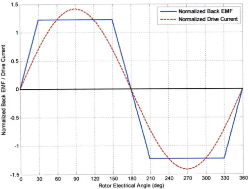
It is certainly possible to mix trapezoidal EMF with sinusoidal drive, or vice versa. Torque production will still occur by the same fundamental mechanism, namely power converted as current is driven into the back EMF. It is possible to analyze the torque production in this mixed case using the same motor model. The specific case considered is sinusoidal drive current with an ideal 1200 trapezoidal back EMF.

In this case, a sinusoidal current is driven into the trapezoidal back EMF. This implies a high-bandwidth current controller that generates whatever voltage is necessary on the phase to keep the current exactly sinusoidal. Figure 9 shows this case, with the RMS-normalized waveforms. The instantaneous power is still the product of current and back EMF, and the average power is still the average value of this product over one electrical cycle. In this case, using the same RMS-normalized back EMF and current waveforms as in Section 2.2.3, the RMS-normalized average power

(20)

output from three phases is 3.15. The power (and torque) now have ripple, as shown in Figure 10. 1.5 -NM Norm -- --- --- Norm---- - A - --- --- --- --- --- --- --- --120 150 180 210 240 27

Rotor Electrical Angle (deg)

alized Back EMF alized Drae Current

0 300 330 360

Figure 9: An ideal 1200 trapezoidal back EMF with sinusoidal drive current, both normalized to RMS = 1.

- I I I -0.5 -1.5 0 30 60 90

(21)

4

a.

01

0 30 60 90 120 150 180 210 240 270 300 330 360

Rotor Electrical Angle

Figure 10: The normalized power output of a sinusoidal drive current into an ideal 120* trapezoidal back EMF. The power and torque contain ripple at six times the electrical frequency.

One subtlety of this analysis is the assumption of sinusoidal drive current, not drive voltage. This requires a high-bandwidth current controller on each phase, which is possible but may not be the most practical solution. Simpler solutions that generate a sinusoidal drive voltage can also be implemented, as discussed in Section 4. The resulting drive current would no longer be a pure sinusoid, but the exact effect on torque ripple is not obvious due to the trapezoidal back EMF.

2.2.5 DC vs. AC Summary

Although the same physical principles apply to both, the definitions of brushless DC and

synchronous AC motors are often confusing. Brushless DC (BLDC) is the term typically applied to motors with a more trapezoidal back EMF, driven by six-step square wave commutation.

Synchronous AC, permanent magnet AC (PMAC), and permanent magnet synchronous motor (PMSM) are all terms typically applied to motors with sinusoidal back EMF being driven by sinusoidal currents. Thus, the definition depends both on the motor and on the drive. It is also possible to mix trapezoidal back EMF with sinusoidal drive, or sinusoidal back EMF with six-step commutation. The fundamental mechanism of torque production is the same, but the average and instantaneous power can differ slightly.

Table 2 summarizes the three cases explored in this section: pure BLDC, pure synchronous AC, and a mix of trapezoidal back EMF with sinusoidal drive current. The relative power (torque) production of each case is normalized to a physical constraint: heat dissipation in the motor. This is done by setting the RMS value of all the drive and back EMF waveforms equal to 1. This is not an exhaustive analysis, since there are any number of back EMF shapes that aren't pure sinusoidal or trapezoidal, as well as other drive combinations. These three cases are also all

(22)

analyzed absent motor inductance, which can greatly change the story. A complete

understanding of the relative performance of DC vs. AC drive for a given motor (specific back EMF, resistance, and inductance) would only be possible with simulation.

Table 2: A summary of the three combinations of back EMF and drive waveforms considered in this section, including the standard BLDC and PMSMIPMAC cases, plus a mixed case.

Normalized Power/ Power/Torque Comments

Torque (x3 Phases) Ripple?

Sinusoidal Back EMF 3.00 No PMSM / PMAC

Sinusoidal Drive No ripple, even with inductance.

120* Trapezoidal Back EMF 3.15 No* BLDC. *Ripple-free only in the

Six-Step Square Wave Drive ideal case with no inductance.

1200 Trapezoidal Back EMF 3.15 Yes, ~ 17%

Sinusoidal Drive

The take-away from Table 2 might be that the difference between AC and DC is not as great as one might think. Under ideal conditions, both synchronous AC and brushless DC motors can produce nearly the same torque per unit heat dissipation, and with relatively little ripple. Brushless DC usually has a slight edge in torque production and achievable speed for a given voltage. However, AC drive with sinusoidal back EMF remains ripple-free even in the presence of inductance, while brushless DC does not (high frequency components of the drive current get filtered out). As the motor inductance and/or speed increase, the benefits of synchronous AC become greater. In the next section, field-oriented control of synchronous AC motors will be presented as a way to further accommodate for motor inductance in the sinusoidal case.

2.3 Field-Oriented Control

Field-oriented control (FOC) is an advanced control technique used primarily for AC induction motors and permanent magnet synchronous motors. It has the advantage of isolating the torque-producing component of motor current from the field-augmenting or field-weakening

component. This allows for a simple and independent torque controller and field controller, as would be the case with a separately-excited DC motor. Field-oriented control is not synonymous with space vector modulation (SVM), sinusoidal commutation, or phase advance, though all or some of these other techniques may be used to achieve field-oriented control.

This report will focus on field-oriented control as it applies to permanent magnet synchronous motors. In PMSM, it is very easy to isolates the torque-producing component of motor current by working in the rotating reference frame of the rotor, which is called the d-q reference frame. Motor quantities can be mapped into the d-q frame by simple trigonometry, and current (torque, field) control can be executed in this frame. This control method is called a synchronous current regulator. Though it is computationally intensive, one goal of this report is to highlight ways to do this efficiently on low-cost hardware. A modified synchronous current regulator optimized for computational efficiency is presented in Section 4.5.

2.3.1 d-q Reference Frame

Essential to field-oriented control in PMSM is the establishment of a frame of reference that is fixed with respect to the rotor. Even simple BLDC controllers accomplish this, to some extent,

by using Hall effect sensors or back EMF sensing to estimate rotor position. Field-oriented

(23)

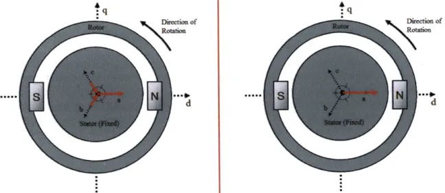
rotating frame. The rotating frame is defined by two axes, labeled direct (d) and quadrature (q) and fixed to the rotor as illustrated in Figure 11. (An outside rotor is used to facilitate the illustration.)

q

d

Figure 11: The d-q reference frame is fixed to the rotor such that the d-axis always falls on the magnetic axis and the q-axis always falls in between the magnetic axis, 900 ahead in the direction of rotation.

The direct (d) axis is defined to be on the magnetic axis passing through the center of a set of permanent magnets on the rotor. The quadrature (q) axis is defined to be 900 electrical ahead of the q-axis in the direction of rotation. In other words, the q-axis always falls exactly between two magnets. In the case of a two-pole motor, this is identical to 90* mechanical, and the axes are physically orthogonal. For higher pole counts, the axes are not physically orthogonal. For example, in a four-pole motor, they are separated by 45* mechanical. For simplicity, the

two-pole, outside rotor illustration in Figure 11 will be used throughout this section. Since motor quantities will be projected based on electrical angle measurements, the number of poles does not affect the control strategy.

2.3.2 Vector Motor Quantities

With the d- and q-axis defined, any motor quantity that has a direction associated with it can be mapped to a vector in the d-q frame by projection. Many motor quantities, including current, are associated with the motor phase windings, which reside on the stator. These quantities take as their direction the principal axis of that phase winding. The three phases (a, b, c) are almost always established at intervals of 1200 electrical to each other. These phase axes are added to the illustration in Figure 12. While the d- and q-axis rotate, the a-, b-, and c-axis stay fixed to the stator.

(24)

Direction of

Rotaion

Figure 12: The three phase winding of the motor defines three equally-spaced axes that are fixed to the stator, labeled a, b, and c.

For example, consider the following balanced set of phase currents:

Ia =lOA Ib = -5A

IC = -5A

These are illustrated as vectors on the stator in Figure 13. Note that you can also sum the three vectors to get a single resultant current vector. (All the tricks of vector geometry apply here.)

Dection of

d

Drecton of

d

Figure 13: The balanced phase currents can be represented as vectors on the stator (left). They can also be summed into one resultant current vector (right).

The magnitude of the resultant vector is calculated as follows: Direction of

Rotaion

(25)

|I=

I+ I| cos(600) +

|I I

cos(600) =15A

3

2

This factor of 3/2, which appears frequently with balanced three-phase quantities, will be important to the analysis. However, different transformations from (ab,c) to (d,q) may or may not account for this factor. Thus, magnitude is deemphasized for now and the focus will be on

the direction of the resultant.

In Figure 13, it is easy to see how the current vector would be mapped onto the d- and q-axis. (Id is positive, Iq is zero.) By considering the current vector as the principal axis of a coil of wire on the stator, the resulting interaction between the rotor and the stator is intuitively clear. The stator becomes like an electromagnet, with its poles along the axis of the resultant current vector. Since the stator electromagnet and the rotor permanent magnet axes are already aligned in Figure 13, there will be no torque produced. (Given the assumption that the d-axis points from south to north, it is the stable point. Otherwise, it would be the anti-stable point. This directional convention is not crucial to the analysis.)

Although it might be obvious, a detailed look at where to place current in the d-q frame for maximum torque is now presented. First, two other motor quantities are mapped in the d-q frame. These are the flux generated by the permanent magnets on the rotor, and the back EMF that flux creates in the motor coils. These two vectors are plotted in Figure 14.

q

Direction of

Rotation

d

Figure 14: Flux caused by the permanent magnets will always align with the d-axis. Back EMF will always lead

this flux by 900 electrical.

The link between permanent magnet flux and back EMF is based on the fundamental formula for back voltage created on a coil of wire in a varying magnetic field:

(26)

E= d .

dt

In the case of a sinusoidal time-varying flux, A, the back EMF, E, will also be sinusoidal and will lead the flux by 900. This is the condition illustrated in Figure 14, with the flux and back EMF vectors representing the instantaneous location of the peak flux and back EMF. These peaks will rotate with the d-q frame such that A is always on the d-axis and E is always on the q-axis. Since the flux considered is from permanent magnets only, this is true regardless of stator current. Given a rotor angular velocity, the magnitude of E is fixed by the motor constant. To convert as much power as possible with a given current, the dot product of the I and E vectors should be maximized. This occurs when current is on the q-axis exclusively. Maximizing power is the same as maximizing torque, since the speed is given. This analysis works as well in the limit as speed goes to zero. Thus, peak torque will always occur when current is on the q-axis.

2.3.3 Why Control is Necessary: Motor Inductance

The fundamental reason why field-oriented control is nontrivial stems from the nature of motor controllers themselves. Most often, they are created with elements that can be modeled as

voltage sources. A set of two switching power devices creates a time-averaged voltage applied to each motor phase. This is an open-loop phenomenon: the voltage is exactly set by controlling the duty cycle of the two switching power devices.

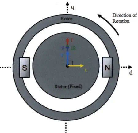
Torque production, however, is governed by current, not voltage. If a motor winding were well-modeled as a simple resistor, there would be no challenge to aligning current on the q-axis. Wherever the rotor is, the phase voltages could simply be set to produce a voltage vector on the

q-axis. With no inductance, that would also be the direction of the current vector. This unrealistic scenario is shown in vector form in Figure 11 Figure 15. The broken-line vector represents the voltage across the winding resistance, which is the difference between V and E.

(27)

Dirction of Rotation

wagon

d

Figure 15: This is what the essential motor quantities would look like in the absence of winding inductance. Voltage, current, and back EMF could all be easily aligned open-loop for maximum torque at any given rotor position.

A real motor, however, has some inductance. Inductors resist changes in current according to the

constitutive equation:

dI

VL = L .

dt

Thus some voltage will be developed across the winding inductance that resists changes in current. If an inductor is subjected to a sinusoidal time-varying voltage, the current will also be sinusoidal and will lag the voltage by 90*.

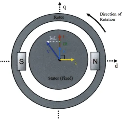
To the extent which they are sinusoidal time-varying quantities, all of the motor quantities can be represented as complex variables to capture the mathematical relationships between voltage, current, resistance, inductance, flux, and back EMF. However, the important effects are more intuitively captured in the relationships between vectors on the d-q frame. For example, if the voltage were fixed to be on the q-axis, Figure 6 shows what effect inductance might have on the current.

... .... . .

(28)

q

Dietion of Rotation

d

Figure 16: The vector relationships between motor quantities if the applied voltage is fixed to the q-axis, but there is inductance present.

Current now lags voltage, due to the inductance. The two broken-line vectors represent components of voltage across the winding resistance and winding inductance. The resistance component is parallel to current and the inductance component leads current by 90*. (In other words, current lags voltage across the inductor by 90*.) The vector sum of voltages is consistent with kitchoff's Voltage Law (KVL).

In Figure 16, current and back EMF are no longer aligned, so torque is not maximized. Open-loop phase advance is one possible way to accommodate for the affect of inductance: Simply placifig vdltage ahead of the q-axis by some angle (which could be a function of other motor paratiitteis, measured or known) could offset most, if not all, of the angle lost to inductance. However, any solution based on open-loop phase advance would be motor-specific. Field-oriented control seeks a more flexible solution based on real-time current measurements.

2.3.4 lid-Oriented Control Objectiv

The objective of field-oriented control is to achieve measurement and closed-loop control of the motor current vector, essentially placing it on the d-q plane. The controller presented is general enough to place the vector anywhere, including leading the q-axis to achieve field weakening. For the most part, though, this report will focus on placing the current veetor on the q-axis, to optimize torque. Figure 17 shows the vector motor quantities might look like with the current vector controlled to be on the q-axis.

(29)

Dirtion of Rotation

d

Figure 17: With current controlled to be on the q-axis, the voltage must lead the back EMF to account for inductance.

The voltage vector is advanced ahead of the back EMF. (In other words, Vd is negative.) This counteracts the lag introduced by motor inductance. Current still lags applied, but it is now in phase with back EMF, producing optimal torque. The broken-line vectors represent the components of voltage across the winding resistance and inductance needed to satisfy KVL. Here it is clear that if the product of current, speed, and inductance is sufficiently small as to be negligible, the degenerate case is that of Figure 15. This product (normalized to the applied voltage) can be used as a test for whether field-oriented control is justified for a given motor and operating range.

2.3.5 Synchronous Current Regulator

The synchronous current regulator is a closed-loop current controller operating in the d-q reference frame. It relies on the ability to transform control quantities readily between the stator (a,b,c) frame and rotor (d,q) frame. To do the projections required for this transformation, the rotor position must be known. All control is done on quantities in the d-q frame, even though the measurements and outputs are done in the stationary frame. Figure 18 shows the standard

synchronous current regulator block diagram.

(30)

Rotor Position IV - e axis Abe

-Inverse

Park Transform

II

Park Transform'

dq

abC

0

Rotor Position

Figure 18: The standard synchronous current regulator block diagram. Using a measured rotor position, the Park and inverse Park Transforms convert between the stationary and rotating frame.

Current is measured on two of three motor phases. (The third must balance the first two.) The phase currents are projected onto the d-q frame as shown in Section 2.3.2 using the Park

Transform. Id and Iq are compared to reference values representing the desired current vector. (In this case, the desired d-axis current is zero.) The errors are used in standard controllers (e.g. proportional-integral) to generate voltage outputs via pulse width modulation (PWM). These outputs are converted back to the stationary frame with the inverse Park Transform and sent to the power stage, where they set voltages at the motor phases.

(31)

3 Brushless Motor Design and Prototyping Methods

3.1 Design Strategy and Goals

The ability to design motors to fit specific applications is an opportunity that is, in the opinion of the author, highly valuable and yet also not well-known. To most, the process of designing electric motor-based systems involves digging through catalogs of motors, immediately limiting the design space to a set of existing components. By the time this set is filtered by physical constraints and performance requirements, it may leave only a handful of options. Or, it may leave none. Breaking down the black-box status of electric motors to open up new design options is the primary goal of this study.

An important disclaimer: In most engineering situations, designing a custom motor is not called for. The set of commercially-available motors is actually fairly large, the pricing reasonable, and, most importantly, the design cycle time is shorter when components can be off-the-shelf. Only in specific instances where there is a gap in the set of available components is a custom design a viable option. The case study of direct-drive scooter motors is an example of this rare scenario. There is also a significant learning opportunity in designing a custom motor, which may have played an even larger role in the author's motivation to pursue such projects. Learning the benefits and challenges of custom motor design by actually building motors is probably the best way to develop a feel for when such designs are a good option, and when off-the-shelf

components will suffice.

Another goal of this study is to show that, by leveraging modem prototyping and analysis techniques and following simple design guidelines, the cost (in time and money) of designing a custom motor is greatly reduced. The above disclaimer notwithstanding, this may tip the balance in favor of a custom design in some instances. Analysis techniques which are useful include combined CAD/FEA using solid modeling and finite element magnetic simulation. This, with some first-order analysis, can give accurate motor performance predictions. CAM and rapid prototyping, using tools such as laser cutting and abrasive water jet machining, can make custom motor fabrication cost- and time-effective even in single quantities. Simple design guidelines that aid assembly (particularly for hand winding and magnet placement) can greatly speed up the process. Lastly, evaluation techniques that don't require expensive equipment can quickly confirm motor performance. All of these techniques, applied at the "alpha prototype" phase, can help prove a motor design and secure resources for further development using more conventional analysis, tooling, and evaluation techniques.

In summary, the goals of this design study are to:

1. Evaluate the conditions under which a custom motor design may be called for, and how

these conditions are affected by the availability of modem prototyping tools. Two case studies will be presented for which a custom motor design could be justified.

2. Demystify the design of custom brushless motors by showing simple analysis and simulation techniques as applied to the case studies.

3. Provide, though the case studies, some examples of modem rapid prototyping techniques

(32)

4. Provide, through the case studies, good design practices that facilitate in-house motor assembly with no special tooling.

5. _{Evaluate whether the motors designed in the case studies meet requirements. If they do}

not, provide means to reconciling the measured performance with analysis and improve the design in future iterations.

3.2 Introduction of Case Studies

Two case studies will be used in this section as real-life examples of custom motor design. The motors built for these two case studies are very different in scale and purpose. However, one goal of this section is to highlight some similarities in their design and prototyping methods.

Wherever possible, the analytical methods will be applied to both cases to show the flexibility of motor analysis. Both motors also take advantage of rapid prototyping methods and design for assembly. Finally, the measured results are compared to analyses to evaluate the motors in each case and qualify the designs (with suggestions for future improvements).

3.2.1 Direct-Drive Kick Scooter Motors

The first case study involves direct-drive electric scooter motors. For large, seated scooters and bicycles, there are a variety of commercial options for in-wheel motors. However, there are no commercially available in-wheel motors for small stand-on "kick scooters," such as Razor scooters. A typical electric kick scooter might have a high-speed motor geared down by belt or chain to the rear wheel. Some benefits of an in-wheel motor include space efficiency, a minimum number of moving parts, no transmission losses, and a cleaner aesthetic more closely resembling an unpowered scooter. Some disadvantages include more complex control, coupling of an expensive component to one normally considered consumable, and exposure of the motor to vibration, dirt, and water.

Without the opportunity for gear reduction, the primary challenge of creating an in-wheel scooter motor is generating sufficient traction force in the direct-drive application. With no gear ratio to work with, and assuming a fixed ratio between the air gap and outer diameters, the force exerted

by the wheel will scale linearly with motor current and length based on ILxB. Motor current, in

turn, scales linearly with copper cross-sectional area. Roughly speaking, then, the force exerted will scale with the volume (length x area) of the in-wheel motor. So, a small wheel motor might need all the design help it can get to generate sufficient force to move a person.

The author cannot claim complete novelty of this design challenge. In fact, this project started with an inspirational proof of concept: a functional razor scooter-sized wheel motor built by Charles Guan '11, shown in Figure 19.

(33)

Figure 19: A Razor scooter-sized wheel motor bu

According to the project documentation [7], this wheel motor achieves a top speed of 15mph (6.7m/s) with a wheel outer diameter of 125mm and a 29.6V battery. A rough calculation of the motor constant, K,, if this is considered the "no-load" speed goes as follows:

V 29.6V V Nm

K, ~ = - 0.28--=0.28-.

(W

6.7 7l

s4

A

0.0625m)

Assuming 30A as a reasonable short-duration current for the magnet wire used to wind this motor, this value for the motor constant would yield a force at the ground of:

K1 I

(

NmY 30A A 1N

F =-'-= 0.28 =134N.

r A 0.0625m)

This force estimate, equal to 301bf, is about 1/5* the weight of a scooter and rider (0.2g

acceleration). This seems like a reasonable traction force. The analysis is crude, but the fact that the scooter works is also convincing evidence that the force is sufficient.

Guan's wheel motor is designed for sensorless commutation, in which the controller detects rotor position by sensing back EMF on an unpowered phase of the motor. This requires some initial speed to lock in, so the scooter needs a kick-start. This is just one example of how the motor, controller, and system design are linked, a theme that will come up many times in this report. During the summer of 2009, the author led a project with the MIT Edgerton Center's Summer Engineering Workshop to create an electric kick scooter with direct-drive motors in both wheels. This project, named the "B.W.D. Scooter" (for Both Wheel Drive) was the author's first

experience with brushless motor design. The B.W.D. Scooter, in finished form, is shown in Figure 20. This case study will track the design goals and prototyping methods that produced the front and rear motors, which differ only in number of turns per phase.

Design and prototyping methods for brushless motors and motor control

Design and Prototyping Methods for Brushless Motors

and Motor Control

ARCHivES

SEP 0

1

2010

LIBRARIES

Design and Prototyping Methods for Brushless Motors

and Motor Control

Table of Contents

I

Introduction

1.1 Project Motivation

1.2 Acknowledgments

2 Fundamentals and Relevant Physical Principles

2.1 Brushless Motor Terminology and Types

2.1.1 Basic Terminology

Stator

Permanent Magnet

12-Slot Stator (Outside Rotor)

Permanent Magnet

Winding

180* Mechanical

360* Electrical

2.1.2 IVotor Model, Back EMF, Motor Constant

Inside Motor:

Brushed DC Motor Model

Inside

Motor:

L

Ideal Transfomer

Ideal

Transfomer

Ideal Transfomer

t

(Oe

+

)m

-- E = K,(0,+

r,

u~:

2.1.3 Resistance, Inductance, Saliency, and Field Weakening

L, =

2.2 DC vs. AC: Back EMF, Drive, and Torque Production

2.2.1 Trapezoidal vs. Sinusoidal Back EMF

kMF

2.2.2 Square Wave vs. Sine Wave Drive

2.2.3 Torque Production Comparison

2.2.4 Mixed Back EMF /

Drive

2.2.5 DC vs. AC Summary

2.3 Field-Oriented Control

2.3.1 d-q Reference Frame

2.3.2 Vector Motor Quantities

|I=

|I I

Direction of

2.3.3 Why Control is Necessary: Motor Inductance

d

d

2.3.4 lid-Oriented Control Objectiv

d

2.3.5 Synchronous Current Regulator

-Inverse

Park Transform

Park Transform'

dq

abC

0

3 Brushless Motor Design and Prototyping Methods

3.1 Design Strategy and Goals

3.2 Introduction of Case Studies

3.2.1 Direct-Drive Kick Scooter Motors

(W

6.7 7l

s4

A

(

**180* Mechanical**

**360* Electrical**