HAL Id: inserm-00540501
https://www.hal.inserm.fr/inserm-00540501
Submitted on 3 Dec 2010
HAL is a multi-disciplinary open access
archive for the deposit and dissemination of sci-entific research documents, whether they are pub-lished or not. The documents may come from teaching and research institutions in France or abroad, or from public or private research centers.
L’archive ouverte pluridisciplinaire HAL, est destinée au dépôt et à la diffusion de documents scientifiques de niveau recherche, publiés ou non, émanant des établissements d’enseignement et de recherche français ou étrangers, des laboratoires publics ou privés.
signals based on pairwise and multivariate analysis.
Chufeng Yang, Régine Le Bouquin Jeannes, Gérard Faucon, Fabrice Wendling
To cite this version:
Chufeng Yang, Régine Le Bouquin Jeannes, Gérard Faucon, Fabrice Wendling. Detecting causal interdependence in simulated neural signals based on pairwise and multivariate analysis.. Confer-ence proceedings : .. Annual International ConferConfer-ence of the IEEE Engineering in Medicine and Biology Society. IEEE Engineering in Medicine and Biology Society. Annual Conference, Institute of Electrical and Electronics Engineers (IEEE), 2010, 1, pp.162-5. �10.1109/IEMBS.2010.5627241�. �inserm-00540501�
Abstract—Our objective is to analyze EEG signals recorded
with depth electrodes during seizures in patients with drug-resistant epilepsy. Usually, different phases are observed during the seizure process, including a fast onset activity (FOA). We aim to determine how cerebral structures get involved during this FOA, in particular whether some structure can “drive” some other structures. This paper focuses on a linear Granger causality based measure to detect causal relation of interdependence in multivariate signals generated by a physiology-based model of coupled neuronal populations. When coupling between signals exists, statistical analysis supports the relevance of this index for characterizing the information flow and its direction among neuronal populations.
I. INTRODUCTION
PILEPSY is a neurological disorder characterized by repetitive seizures. In 30% of the cases, seizures remain drug-resistant and considerably affect all aspects of the patient’s life [1]. Drug-resistant epilepsies are often partial, with an epileptogenic zone (EZ) located in a relatively circumscribed brain area. For these partial epilepsies, surgical treatment can be considered. The difficulty that arises is then to determine the organization of the EZ and, thus, the areas that should be removed in order to suppress seizures. In some patients, the pre-surgical evaluation may include recording of intracerebral electroencephalographic (iEEG) signals using depth electrodes. The analysis of such signals remains a difficult task aimed at determining which sites of the brain belong to the EZ, prior to surgery. In this context, signal processing techniques can provide some quantitative information that cannot be easily obtained by visual analysis. This is typically the case for correlation (wide-sense) measures that proved useful for assessment of functional couplings between distant brain sites [2]. In this paper, we present some evaluation results about a method allowing for determination of causality relationships among neuronal ensembles from signals produced by these ensembles (typically local field potentials or iEEG signals). The concept of causality between time series was first introduced by Wiener [3] in 1956, then formulated by Granger [4] and known as Granger Causality Index (GCI). Granger causality is a statistical concept of causality that is
Manuscript received April 23, 2010. This work was supported by China Scholarship Council (CSC) under Grant No. 2008609145. C. Yang, R. Le Bouquin Jeannès, G. Faucon, and F. Wendling are with INSERM, U642, Rennes, F-35000, France; Université de Rennes 1, LTSI, F-35000, France. Corresponding author: R. Le Bouquin Jeannès, phone: 33-(0)2-23236919; fax: 33-(0)2-23236917; e-mail: [email protected].
based on prediction and has been widely used in economics since the 1960s. According to Granger causality, if a signal
1
x "causes" a signal x2, then past values of x1 should contain information that helps predict x2 above and beyond the information contained in past values of x2 alone. If GCI
is an effective tool to describe causal interactions between signals, it is only within the last few years that applications in neuroscience have become popular [5]-[7]. In this paper, the method is evaluated on signals simulated from physiology-based model of coupled neuronal populations in which causality relationships can be controlled. The key features of this model are two-fold. First, it generates signals for which properties are similar to those of real signals observed at the onset of epileptic seizures. Second, it provides a “ground truth” about the degree and direction of couplings between populations of neurons, which is hardly accessible on real data.
II. MATERIAL AND METHODS
A. Linear Granger Causality Index (LGCI)
Granger causality is normally tested in the context of linear regression models. Let x1,…, xQ be Q zero-mean
signals whose discrete-time observations are noted
1( ), ( ),..., ( )2 Q
x t x t x t , t=1, 2,...,T , where T is the signal length. If we model the observations by a multivariate autoregressive (AR) model of order m , we write
( )
( )
(
)
(
)
( )
( )
1 1 1 1 -m k k Q Q Q x t x t k w t A x t = x t k w t ⎡ ⎤ ⎡ ⎤ ⎡ ⎤ ⎢ ⎥ = ⎢ ⎥ + ⎢ ⎥ ⎢ ⎥ ⎢ ⎥ ⎢ ⎥ ⎢ ⎥ ⎢ ⎥ ⎢ ⎥ ⎣ ⎦ ⎣ ⎦ ⎣ ⎦∑
# # # (1)where each signal depends not only on its own past but also on the past of the other signals. w ti( ), i=1, 2,..., Q, are white Gaussian noises, and
( )
( )
( )
( )
( )
( )
1.1 1.2 1. . .1 . Q i j k Q Q Q k k k k A k k α α α α α α ⎡ ⎤ ⎢ ⎥ ⎢ ⎥ ⎢ ⎥ = ⎢ ⎥ ⎢ ⎥ ⎢ ⎥ ⎢ ⎥ ⎣ ⎦ " " # # # # # # # # # # # # # # " " " . (2)Detecting causal interdependence in simulated neural signals based
on pairwise and multivariate analysis
C. Yang, R. Le Bouquin Jeannès, G. Faucon, and F. Wendling
The coefficient α.i j
( )
k evaluates the linear interaction of(
)
j
x t k− on x ti
( )
, whatever i j, . These coefficients are estimated by solving Yule–Walker equations.Let us begin with the case of two signals by studying the causality x1→x2. From an univariate model, the quality of the representation of x2 may be evaluated from the variance
of the prediction error
2 2| −
Γx x , where x2− symbolizes x2 past. Using a bivariate model, the variance of the prediction error becomes
2 2| ,− 1−
Γx x x . If x1 causes x2 in the Granger
sense, then
2 2| ,− 1−
Γx x x is smaller than
2 2| −
Γx x . Considering pairwise analysis, the level of LGCI from x1 to x2 is then evaluated by 2 2 2 2 1 | 12 | , LGC I -P ln − − − Γ = Γ x x x x x . (3) Reciprocally, the LGCI from x2 to x1 can be evaluated.
In the case of multiple signals, we can analyze independently each pair of signals as previously. However, pairwise analysis in this multivariate case cannot distinguish between direct and indirect coupling. In the multivariate case, to disambiguate such cases, direct causality from xi to
j
x conditionally to other signals is noted LGCI -Mij and defined by (4) where the numerator is the variance of the prediction error of xj by taking all signals into account except xi 1 1 1 1 | | LGC I -M ln − − − − − + − − Γ = Γ " " " j i i Q j Q x x x x x ij x x x . (4)
B. Model of iEEG Signals Generation
We used a physiology-based model to simulate the field activity of distant - and possibly coupled - neuronal populations. Each population generates a local activity that can be considered as an iEEG signal if one does not consider the source-electrode quasi-static transfer function. Readers may refer to [8], [9] for more information. In the model, each population contains three subpopulations of neurons that mutually interact via excitatory or inhibitory feedback: main pyramidal cells and two types of local interneurons. Since pyramidal cells are excitatory neurons that project their axons to other areas of the brain, the model accounts for this organization by using the average pulse density of action potentials from the main cells of one population i as an excitatory input to another population j. In addition, this connection from population i to j is characterized by parameter K which represents the degree of coupling ij
associated with this connection. Appropriate setting of parameters Kij allows for building systems where the
neuronal populations are unidirectionally or bidirectionally coupled. Other parameters include excitatory and inhibitory gains in feedback loops as well as average number of synaptic contacts between subpopulations. These parameters are adjusted to control the intrinsic activity of each population (normal background versus epileptic activity).
C. Simulated Signals
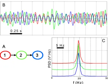
The model described above was used to simulate long duration signals (400 s) for a fixed connectivity pattern among neuronal populations, as illustrated in Fig. 1A and Fig. 1B. Sampling rate was equal to 256 Hz. Model parameters were such that: (i) a fast quasi-sinusoidal (25 Hz, Fig. 1C) activity (similar to that observed at seizure onset) was generated by the three populations when they were uni-directionally coupled (1Æ2Æ3) and (ii) this fast onset activity was only generated by population 1 when they were uncoupled. In this second situation, populations 2 and 3 generated normal background activity (not shown).
This scenario ensured that the epileptic activity present in populations 2 and 3 was caused by that of population 1. Another key aspect is that the spectral features of output signals are very close under the “coupled” condition. In addition, some jitter might be observed between simulated time series (Fig. 1B) as also observed in real situations, at seizure onset.
III. RESULTS
In this section, we present results on (i) LGCI in presence or absence of coupling, (ii) the influence of coupling strength. For the experiments, when there is a coupling between observations, the coupling coefficients are chosen identical, i.e. K12=K23= . Model order m is estimated K by minimizing the Akaike's information criterion (AIC) on each frame. 1 2 3 0 5 0 5 H z 0 .2 5 s 2 5 A B C f (H z ) PSD (V ². H z) 1 2 3 11 2 33 0 5 0 5 H z 0 .2 5 s 2 5 A B C f (H z ) PSD (V ². H z)
Fig. 1. Simulated signals. A. Considered scenario for connectivity among neuronal populations. Epileptic activity in population 2 (resp. 3) is caused by excitatory drive from population 1 (resp. 2). B. An example of output signals when populations are coupled. Time delays are not constant over time. C. Power spectral densities (PSD) of the signals are similar and match those observed in depth-EEG signals at the onset of seizures.
A. Detection of Information Flow
Firstly, we estimate LGCI considering pairwise analysis of signals (LGCI-P) and multivariate analysis (LGCI-M). The indices depend on the coupling and on the signals under study. LGCI is performed on 1024-point adjacent frames corresponding to sequences of 4s time duration, which is suitable for real signals (estimating changes below this value appears more difficult). For our simulated signals, we obtain 100 values of indices. Table I reports the averaged indices for K= and 0 K=1500. For K= , on the one hand, the 0 averaged LGCI-P are similar (about 0.005) and, on the other hand, the averaged LGCI-M are also similar (about 0.003). Now, let us consider a coupling between signals using
1500
K= . As expected, LGCI from x1 to x2 and from x2
to x3 increase, both in pairwise and multivariate analysis. For each index, the variation (without coupling vs with coupling) is comparable using LGCI-P or LGCI-M (around 0.015 for LGCI12, and around 0.005 for LGCI23). This finding means that detecting the flow x2→x3 is more difficult than detecting the flow x1→x2. As for the relation
1 3
x →x , it is indirect and completely mediated by signal 2
x . Consequently, when K=1500, LGCI -M13 remains at a low value (0.0039 vs 0.0031) since it is based on a multivariate analysis. Fitting a two-dimensional AR model, the LGCI -P13 index, which should have risen, does not sufficiently increase to reveal an influence from x1 to x3. Let us note that all other indices, corresponding to the opposite directions x2→x1, x3→x2 and x3→ , remain x1 low and quite constant in both conditions and present a lower variation using multivariate analysis. According to these remarks, we displayed on Fig. 2 the time evolution of
12
LGCI -M and LGCI -M21 , for K=1500, showing that
12
LGCI -M is generally greater than LGCI -M21 . To confirm these results, statistical significance has to be addressed.
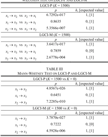
Statistical analysis on LGCI-P and LGCI-M is summarized in Tables II and III. In these tables, the last column gives the value of the hypothesis test (a value of 1 indicates that the null-hypothesis is rejected) and the expected value according to our scenario is given into brackets. In Table II, we test whether LGCI computed from signal i to signal j is significantly different from LGCI computed from signal j to signal i using the Wilcoxon signed-rank test. The unidirectional information flow from signal 1 to signal 2 is obvious with a very low p-value for
pairwise or multivariate analysis (lower than 1e-16). In the same way, we can conclude on the information flow from signal 2 to signal 3 with a p-value at least lower than 1e-3.
TABLEI
RESULTS ON LGCI-P AND LGCI-M LGCI-P i j x →x i = 1 i = 2 i = 3 j = 1 - 0.0054 0.0048 j = 2 0.0055 - 0.0046 0 K= j = 3 0.0052 0.0047 - i j x →x i = 1 i = 2 i = 3 j = 1 - 0.0064 0.0058 j = 2 0.0209 - 0.0062 1500 K= j = 3 0.0059 0.0107 - LGCI-M i j x →x i = 1 i = 2 i = 3 j = 1 - 0.0034 0.0031 j = 2 0.0032 - 0.0029 0 K= j = 3 0.0031 0.0031 - i j x →x i = 1 i = 2 i = 3 j = 1 - 0.0034 0.0036 j = 2 0.0183 - 0.0046 1500 K= j = 3 0.0039 0.0071 - TABLEII
WILCOXON TEST ON LGCI-P AND LGCI-M LGCI-P (K = 1500) p h, [expected value] 1 2 x →x vs x2→x1 6.7292e-017 1, [1] 1 3 x →x vs x3→x1 0.8635 0, [1] 2 3 x →x vs x3→x2 5.3566e-007 1, [1] LGCI-M (K = 1500) p h, [expected value] 1 2 x →x vs x2→x1 3.6417e-017 1, [1] 1 3 x →x vs x3→x1 0.7859 0, [0] 2 3 x →x vs x3→x2 2.6778e-004 1, [1] TABLEIII
MANN-WHITNEY TEST ON LGCI-P AND LGCI-M LGCI-P (K = 1500 vs K = 0) p h, [expected value] 1 2 x →x 4.8567e-026 1, [1] 1 3 x →x 0.6451 0, [1] 2 3 x →x 7.2285e-010 1, [1] LGCI-M (K = 1500 vs K = 0) p h, [expected value] 1 2 x →x 3.7870e-027 1, [1] 1 3 x →x 0.7222 0, [0] 2 3 x →x 4.5928e-006 1, [1] 20 40 60 80 100 -0.01 0 0.0034 0.0183 0.05 Frames LG C I-M LGCI21-M LGCI 12-M
Fig. 2. LGCI12-M (K=1500) (solid line) versus LGCI21-M (K=1500)
For both indices, the only difference relies on the information flow from signal 1 to signal 3. For LGCI-M, the result is coherent: there is no direct relation between the two signals. As for LGCI-P, since signals are studied by pairs, we must find information flow from signal 1 to 3 but we can notice that the index fails in this case (h= ). 0
The second test, presented in Table III, consists in pointing out the effective coupling between signals when the parameter K turns from 0 to 1500. Estimators are tested only for the real causal relations (either direct or indirect). It comes out that, in each case, using either P or LGCI-M, the Mann-Whitney test reveals a coupling from signal 1 to signal 2, and from signal 2 to signal 3. As previously, the interaction from signal 1 to signal 3 cannot be put forward using LGCI-P, whereas it should be the case. On the other hand, LGCI-M does not reject the null-hypothesis since there is no direct relation between populations 1 and 3.
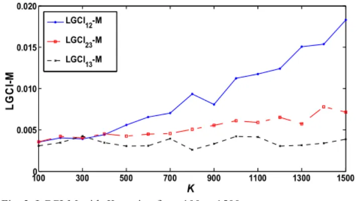
B. Variable Coupling
In this section, we study the significant influence of the coupling parameter K on LGCI in the vectorial case. Fig. 3 shows the evolution of LGCI -M12 , LGCI -M23 and
13
LGCI -M, when K varies from 100 to 1500 by step of 100. LGCI -M12 and LGCI -M23 vary linearly with K
(with a steeper slope for LGCI -M12 ) while LGCI -M13 is quite stable. So, the directions x1→x2 and x2→x3 are
easier to detect when K increases.
We first tested the significance of LGCI-M between populations 1 and 2 for a value of K different from 0. The value of h using the Wilcoxon test is plotted in Fig. 4. For a
p-value of 0.05, the test indicates a flow direction from
population 1 to population 2 as soon as K reaches 500. When we test LGCI -M12 without and with coupling ( K varying from 100 to 1500), the Mann-Whitney test indicates a significant difference at a p-value of 0.05, whatever the
value of K , except K = 100 and K = 400. In the same way, significant causality has been tested between populations 2 and 3. Testing LGCI -M23 versus
32
LGCI -M can be sometimes not significant at a level of 5%, even for K greater than 500. Now, testing LGCI -M23 with and without coupling yields a significant difference above K=700.
IV. CONCLUSION
This paper was aimed at better understanding how seizure activity arises from a model of three neuronal populations. The a priori knowledge of effective coupling allows us to
evaluate the relevance of Granger causality indices. The results reported in this paper show that the method can reveal the underlying network organization in a difficult situation where time shifts between signals strongly vary in time, as in the real case. Based on multivariate or pairwise analysis, direct causal relations are well detected for a sufficiently strong coupling whereas pairwise analysis may fail in detecting indirect relations. In a future work, according to the narrow-band characteristics of the signals, we plan to conduct statistical analysis in the frequency domain.
REFERENCES
[1] J. Engel, P. VanNess, T. Rasmussen, and L. Ojemann, “Outcome with respect to epileptic seizures,” in Surgical Treatment of the Epilepsies,
2nd ed. J. Engel, Ed. New York: Raven Press, 1993, pp. 609-622. [2] K. Ansari-Asl, L. Senhadji, J. J. Bellanger, and F. Wendling,
“Quantitative evaluation of linear and nonlinear methods characterizing interdependencies between brain signals," Phys Rev E
Stat Nonlin Soft Matter Phys, 74(3 Pt 1):031916, 2006.
[3] N. Wiener, “The theory of prediction,” in Modern Mathematics for Engineers, vol. 1, E. F. Beckenbach, Ed. New York: McGraw-Hill,
1956, pp. 125–139.
[4] C. W. J. Granger, “Investigating causal relations by econometric models and cross-spectral methods,” Econometrica, vol. 37, pp.
424-438, Aug. 1969.
[5] X. Wang, Y. Chen, S. L. Bressler, and M. Ding, “Granger causality between multiple interdependent neurobiological time series: Blockwise versus pairwise methods,” Int. J. of Neural Systems, vol. 17, pp. 71-78, 2007.
[6] A. S. Kayser, F. T. Sun, and M. D’Esposito, “A comparison of Granger causality and coherency in fMRI-based analysis of the motor system,” Human Brain Mapping, vol. 30, pp. 3475-3494, Nov. 2009. [7] J. Dauwels, F. Vialatte, T. Musha, and A. Cichocki, “A comparative
study of synchrony measures for the early diagnosis of Alzheimer's disease based on EEG,” NeuroImage, vol. 49, pp. 668-693, Jun. 2009. [8] F. Wendling, J. J. Bellanger, F. Bartolomei, and P. Chauvel,
“Relevance of nonlinear lumped-parameter models in the analysis of depth-EEG epileptic signals,” Biological Cybernetics, vol. 83, pp. 367-378, 2000.
[9] F. Wendling, A. Hernandez, J. J. Bellanger, P. Chauvel, and F. Bartolomei, “Interictal to ictal transition in human temporal lobe epilepsy: insights from a computational model of intracerebral EEG,”
J. Clin Neurophysiol, vol. 22, pp. 343-356, 2005.
1000 300 500 700 900 1100 1300 1500 0.005 0.010 0.015 0.020 K LGC I-M LGCI12-M LGCI23-M LGCI 13-M
Fig. 3. LGCI-M with K varying from 100 to 1500.
100 300 500 700 900 1100 1300 1500 0 1 K h LGCI 12-M (K ≠ 0) versus LGCI21-M (K ≠ 0)
LGCI12-M (K ≠ 0) versus LGCI12-M (K = 0)
Fig. 4. LGCI12-M (K≠ ) versus LGCI0 21-M (K≠ ) (solid line) and 0
LGCI12-M (K≠ ) versus LGCI0 12-M (K= ) (dotted line) with K varying 0