DETERMINING THE FLOW DIRECTION OF CAUSAL INTERDEPENDENCE IN MULTIVARIATE TIME SERIES.

HAL Id: hal-00911072

https://hal.archives-ouvertes.fr/hal-00911072

Submitted on 29 Nov 2013

HAL is a multi-disciplinary open access

archive for the deposit and dissemination of

sci-entific research documents, whether they are

pub-lished or not. The documents may come from

teaching and research institutions in France or

abroad, or from public or private research centers.

L’archive ouverte pluridisciplinaire HAL, est

destinée au dépôt et à la diffusion de documents

scientifiques de niveau recherche, publiés ou non,

émanant des établissements d’enseignement et de

recherche français ou étrangers, des laboratoires

publics ou privés.

DETERMINING THE FLOW DIRECTION OF

CAUSAL INTERDEPENDENCE IN MULTIVARIATE

TIME SERIES.

Chunfeng Yang, Régine Le Bouquin Jeannes, Gérard Faucon

To cite this version:

Chunfeng Yang, Régine Le Bouquin Jeannes, Gérard Faucon. DETERMINING THE FLOW

DIREC-TION OF CAUSAL INTERDEPENDENCE IN MULTIVARIATE TIME SERIES.. 18th European

Signal Processing Conference (EUSIPCO), Aug 2010, Aalborg, Denmark. pp.636-640. �hal-00911072�

DETERMINING THE FLOW DIRECTION OF CAUSAL INTERDEPENDENCE IN

MULTIVARIATE TIME SERIES

Chunfeng Yang

1, 2

, Régine Le Bouquin-Jeannès

1, 2

and Gérard Faucon

1, 2

1

INSERM, U 642, Rennes, F-35000, France

2

Université de Rennes 1, LTSI, F-35000, France

Campus de Beaulieu, Bât 22, Université de Rennes 1, 35042, Rennes Cedex, France

phone: + 33 (0)2 23 23 62 20, fax: +33 (0)2 23 23 69 17

email: {chunfeng.yang, regine.le-bouquin-jeannes, gerard.faucon}@univ-rennes1.fr

web: www.ltsi.univ-rennes1.fr

ABSTRACT

Phase slope index is a measure which can detect causal direction of interdependence in multivariate time series. However, this co-herence based method may not distinguish between direct and indirect relations from one time series to another one acting through a third time series. So, in order to identify only direct rela-tions, we propose to replace the ordinary coherence function used in phase slope index with the partial coherence. In a second step, we consider and compare two estimators of the coherence func-tions, the first one based on Fourier transform and the second one on an autoregressive model. These measures are tested and com-pared with Granger causality index on linear and non linear time series. Experimental results support the relevance of the new index including partial coherence based on autoregressive modelling in multivariate time series.

1.

INTRODUCTION

In neuroscience, understanding of brain functioning requires the investigation of activated cortical networks, in particular the detec-tion of interacdetec-tions between different cortical sites. The concept of causality between time series was first introduced by Wiener [1] in 1956, then formulated by Granger [2] and known as Granger Cau-sality Index (GCI). Later, the frequency decomposition of this fun-damental tool was given by Geweke [3, 4]. Over the last decade, other measures have been derived being applied to chaotic systems and multivariate neurobiological signals [5-10]. Furthermore, cross correlation in the time domain and coherence functions in the spec-tral domain were also used to estimate statistical causal relations between neural signals [11-14].

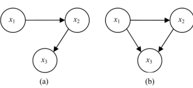
Recently, a measure named Phase Slope Index (PSI) was proposed by Nolte [15, 16] to detect the information flow direction. This method, based on linear phase between two signals, estimates the causal direction by computing the slope of the phase of ordinary coherence function. However, in multivariate time series, when two time series have direct and/or indirect causal relations as in Figure 1, PSI based on ordinary coherence function is not able to distinguish them. In order to detect direct causal relations and dis-tinguish patterns of connectivity as those presented in Figure 1, we recommend a new phase slope index based on partial coherence function instead of ordinary coherence function. Moreover, in [15, 16], ordinary coherence function is obtained using Fourier trans-forms. Another way is to derive the coherences (ordinary and par-tial) by means of autoregressive (AR) modelling of signals as pro-posed hereafter.

Figure 1 – Two patterns of causal interactions (a) causality from signal x1 to x3 is indirect and mediated by x2

(b) both direct and indirect causalities exist from signal x1 to x3.

In the following, phase slope based measures are detailed theoreti-cally. Then, some linear and non linear time series are considered to test them and compare their performance with that of GCI. Finally, some conclusions are drawn.

2.

METHODS

2.1 AR modelling

Let X and ₁ X be two zero-mean signals whose time observations ₂

are noted x t and ₁

( )

x₂

( )

t , with t=1, 2,...,T . If we model each

observation x t and ₁

( )

x₂

( )

t by an univariate AR model of order p, we have

( )

( ) ( ) ( )

1 1 1 1 1 -α = =

_∑

p + k x t k x t k u t (1)

( )

( ) ( )

( )

2 2 2 2 1 -α = =

_∑

p + k x t k x t k u t (2) where each signal, at time t , depends only on its own past, u t ₁

( )

and u₂

( )

t are white Gaussian noises. Now, if we model both

sig-nals x t and ₁

( )

x₂

( )

t by a bivariate AR model of order p, we write

( )

( ) ( )

( ) ( )

( )

1 1.1 1 1.2 2 1 1 1 - -α α = = =

∑

p +

∑

p + k k x t k x t k k x t k w t (3)

( )

( ) ( )

( ) ( )

( )

2 2.2 2 2.1 1 2 1 1 - -α α = = =

∑

p +

∑

p + k k x t k x t k k x t k w t (4) x1 x2 x3 (a) (b) x1 x2 x3

where each signal depends not only on its own past but also on the past of the second signal, w t and ₁

( )

w t are white Gaussian ₂

( )

noises.This model can be extended to Q signals x₁, ,..., x₂ x , with_Q

( )

( )

( )

( )

( )

( )

1 1 1 1 -= ⎡ ⎤ ⎡ ⎤ ⎡ ⎤ ⎢ ⎥ ₌ ⎢ ⎥ ₊ ⎢ ⎥ ⎢ ⎥ ⎢ ⎥ ⎢ ⎥ ⎢ ⎥ ⎢ ⎥ ⎢ ⎥ ⎣ ⎦ ⎣ ⎦ ⎣ ⎦

∑

p k k Q Q Q x t x t k w t A x t x t k w t (5) where

( )

( )

( )

( )

( )

( )

1.1 1.2 1. . .1 . α α α α α α ⎡ ⎤ ⎢ ⎥ ⎢ ⎥ ⎢ ⎥ = ⎢ ⎥ ⎢ ⎥ ⎢ ⎥ ⎢ ⎥ ⎣ ⎦ Q k m n Q Q Q k k k A k k k (6)

The coefficient α_{m n.}

( )

k evaluates the linear interaction of

(

−

)

n

x t k on x_m

( )

t , whatever ,m n . These coefficients are

esti-mated by solving Yule–Walker equations.

2.2 Granger Causality Index (GCI)

GCI proposed by Granger is an effective tool to describe causal interactions between signals. Hereafter, the bivariate case is detailed and extended to the multivariate case.

Let us begin with the case of two signals by studying the causality

1→ 2

x x . From the univariate model given in Eqs. (1) and (2), the quality of the representation of X₂ may be evaluated from the vari-ance of the prediction error

2 2| −

Γ_{x x} , where x2− symbolizes x2 past

( )

(

)

2 2| 2 var − Γ_{x x} = u t (7) where var . denotes the variance. Using the bivariate model of

( )

Eqs. (3) and (4), we have

( )

(

)

2 2| ,1 2 var − − Γ_{x x x} = w t . (8) If X causes ₁ X in the Granger sense, then ₂

2 2|− −,1

Γ_{x x x} is smaller than

2 2| −

Γ_{x x} . The level of Linear Granger Causality Index (LGCI) from X to ₁ X is then evaluated by ₂

2 2 1 2 2 2 1 | | , LGC I ln − − − → Γ = Γ x x x x x x x . (9)

Reciprocally, the LGCI from X to ₂ X can be evaluated. ₁

In the multivariate case, we can analyze independently each pair of signals (pairwise analysis). However, pairwise analysis in the multi-variate case cannot distinguish between direct and indirect coupling. For example, for the two coupling schemes displayed in Figure 1, a pairwise analysis gives the same patterns of connectivity. In the multivariate case, to disambiguate such cases, direct causality from

m

X to X_n conditionally to other signals is defined by Eq. (10) where the numerator is the variance of the prediction error by taking all signals into account except x_m

1 1 1 1 | | LGC I ln − −₋ −₊ − − − → Γ = Γ n m m Q m n n Q x x x x x x x x x x . (10)

2.3 Phase Slope Index (PSI)

PSI is a method to evaluate the direction of information flow in multivariate time series [16]. Hereafter, the principle of PSI method is first recalled. In a second step, partial coherence function is in-troduced to detect only direct relations in multivariate case. Finally, an AR modelling based method for estimating coherence functions is presented.

2.3.1. PSI principle

The basic hypothesis relies on the phase linearity between signals. PSI is based on the slope of the phase of cross-spectrum between two time series x_m

( )

t and x_n

( )

t .

The idea is to define an average phase slope in such a way that this quantity properly represents relative time delays of different signals. This quantity is termed PSI and defined by

( ) (

)

PSI ∗ δ ∈ ⎛ ⎞ ⎜ ⎟ = ℑ_⎜ + _⎟ ⎝

∑

⎠ mn mn mn f F C f C f f (11)

where C_mn

( )

f is the coherence function between signals x and _m

n

x , δf is the frequency resolution, ℑ i denotes taking the

( )

imaginary part and the asterisk denotes conjugate value. F is the set of frequencies over which PSI is computed. In this equation, the coherence function used by Nolte is the ordinary coherence between signals x_m

( )

t and x_n

( )

t , noted as OC_mn

( )

f hereafter, and de-fined by

( )

=

_{( ) ( )}

mn

( )

mn mm nn S f OC f S f S f (12)

where S_mm

( )

f and S_nn

( )

f are the auto-spectral density func-tions of signals x_m

( )

t and x_n

( )

t respectively, and S_mn

( )

f is the

cross-spectral density function. Spectral densities are given by:

( )

⎡

( ) ( )

* ⎤

= ⎣ ⎦

mn m n

S f E X f X f . (13) where X_m

( )

f is the Fourier transform of the signal x_m

( )

t and where E

[ ]

. denotes the expectation. The magnitudes of the coher-ences allow to weight the phase difference between two consecutive frequencies and, consequently, to decrease its impact when the co-herence magnitudes are low. The sign of PSI indicates the flow direction and its magnitude increases along with the delay. Given Eqs. (11) to (13), when the information flow is from x_m

( )

t to

( )

n

x t , PSI_mn is positive. In the following, PSI using the ordinary coherence is named PSI-OC.

2.3.2. PSI using partial coherence

The partial coherence function gives the level of coupling between two signals x_m

( )

t and x_n

( )

t when the influence of the Q

−

2 other signals is removed [12]. It is defined by

( )

_{( )}

2

( )

_{( )}

2 2 2 − − − − ⋅ ⋅ ⋅ ⋅ Q Q Q Q mn X mn X mm X nn X S f PC f S f S f (14) where X_Q−2 x₁ x_m−1x_m+1 x_n−1x_n+1 x_Q .

( )

2 − ⋅ Q mn X S f is the conditioned cross-spectral density function between signals

( )

m x t and x_n

( )

t given X_Q−2,

( )

2 − ⋅ Q mm X S f and

( )

2 − ⋅ Q nn X S f

and x_n

( )

t respectively. In PSI given in Eq. (11), we replace the

ordinary coherence with the partial coherence and the corresponding PSI is noted PSI-PC: the influence of the Q

−

2 other signals is removed and only the direct influence between x_m

( )

t and x_n

( )

t is

considered.

2.3.3. Coherence functions estimators

In Eq. (13), the auto-spectral and cross-spectral density functions may be obtained by two different techniques, either from direct Fourier transforms of signals x_m

( )

t and x_n

( )

t , or from AR

model-ling.

In the first one, the expectation required to get the spectral density functions is obtained by averaging and overlap.

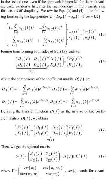
In the second one, even if the approach is intended for the multivari-ate case, we derive hereafter the methodology in the bivarimultivari-ate case for reasons of simplicity. We rewrite Eqs. (3) and (4) in the follow-ing form usfollow-ing the lag operator L

(

Lx_m

( )

t =x_m

( )

t−1 ,m=1, 2

)

( )

( )

( )

( )

( )

( )

( )

( )

1.1 1.2 1 1 1 1 2 2 2.1 2.2 1 1 1 1 p p k k k k p p k k k k k L k L x t w t x t w t k L k L α α α α = = = = ⎛ ⎞ − − ⎜ ⎟ ⎛ ⎞ ⎛ ⎞ ⎜ ⎟_{⎜ ⎟ ⎜= ⎟} ⎜ ⎟⎜_⎝ ⎟ ⎜_{⎠ ⎝} ⎟_⎠ ⎜ _{− −} ⎟ ⎜ ⎟ ⎝ ⎠

∑

∑

∑

∑

(15)

Fourier transforming both sides of Eq. (15) leads to:

( )

( )

( )

( )

( )

( )

( )

( )

( )

11 12 1 1 21 22 2 2 ⎛ ⎞⎛ ⎞ ⎛₌ ⎞ ⎜ ⎟⎜ ⎟ ⎜ ⎟ ⎜ ⎟⎜ ⎟ ⎜ ⎟ ⎝ ⎠⎝ ⎠ ⎝ ⎠ D f D f D f X f W f D f D f X f W f (16)

where the components of the coefficient matrix D f are

( )

( )

( )

2

( )

( )

2 11 1.1 12 1.2 1 1 1 α − π , α − π , = = = −

_∑

p i fk = −

_∑

p i fk k k D f k e D f k e

( )

( )

2

( )

( )

2 21 2.1 22 2.2 1 1 , 1 . π π α − α − = = = −

∑

p i fk = −

∑

p i fk k k D f k e D f k e

Defining the transfer function H f as the inverse of the coeffi-

( )

cient matrix D f , we obtain

( )

( )

( )

( )

( )

( )

( )

( )

( )

( )

1 11 12 1 2 21 22 2 ⎛ ⎞ ⎛₌ ⎞⎛ ⎞ ⎜ ⎟ ⎜ ⎟⎜ ⎟ ⎜ ⎟ ⎜ ⎟⎜ ⎟ ⎝ ⎠ ⎝ ⎠⎝ ⎠ H f X f H f H f W f X f H f H f W f . (17)

Then, we get the spectral matrix

( )

11

( )

_{( )}

12

( )

_{( )}

( )

†

( )

21 22 ⎛ ⎞ =_{⎜ ⎟}= Γ ⎝ ⎠ S f S f S f H f H f S f S f (18) where

( )

(

)

(

21 1

)

( )

12 2 var cov , cov , var ⎛ ⎞ Γ = ⎜ ⎟ ⎝ ⎠ w w w

w w w , cov(.) stands for

covari-ance and † denotes complex conjugate and matrix transposition. Finally, the corresponding PSI-OC can be calculated using Eqs. (11), (12), and (18). Practically, the above algorithm is extended to the multivariate case to get PSI-OC and PSI-PC.

3.

EXPERIMENTAL RESULTS

In this section, two examples of linear and nonlinear stochastic systems are tested. In the first one, we consider a linear stochastic model consisting of three time series simulating (i) the case shown

in Figure 1.a, in which the causal influence from signal x₁ to sig-nal x is indirect and completely mediated by signal ₃ x , (ii) the ₂

case shown in Figure 1.b, containing both direct and indirect causal influences from signal x to signal ₁ x . The second example corre-₃

sponds to the same situations considering non linear signals with linear coupling. For AR modelling, the order is given by Akaike's criterion.

3.1 Linear signals and linear couplings

For the linear stochastic system we consider, the following three signals are generated:

( )

( )

( )

( )

( )

( )

( )

( )

( )

( )

( )

1 1 1 1 2 1 2 3 2 1 3 0.95 2 1 0.9025 2 0.5 1 0.4 2 4 ⎧ = − − − + ⎪ _{= − − +} ⎨ ⎪ _{= − + − +} ⎩ x t x t x t w t x t x t w t x t x t cx t w t (19)

where w tj

( )

,j=1, 2,3, are independent white Gaussian noises with zero means and unit variances, c=0 and c=0.5 are chosen to consider two patterns of causal interactions which include direct and indirect causal relationships as in Figure 1. The sampling fre-quency is 512 Hz. Signals spectra are given in Figure 2, for c=0. The signal x₁ oscillates around 65 Hz as well as x₂ and x₃, due to the flows x₁→x and ₂ x₂→x . ₃

3.1.1. Results on LGCI

Firstly, we estimate LGCI considering pairwise analysis (LGCI-P) and multivariate analysis (LGCI-M). Simulation is carried out 100 times on 1024-point signals, then the means and standard devia-tions (std) are derived and reported in Table 1.

Table 1 – Results on LGCI-P and LGCI-M. The first line indicates the mean, and the second line in parentheses is the standard

devia-tion (std). Reciprocal indices tend to zero and are not displayed. LGCI-P LGCI-M 0 = c 0.5c= c=0 0.5c= 1 2 LGCI_x→x 0.8810 (0.0670) 0.8810 (0.0670) 0.7920 (0.0456) 0.5848 (0.0348) 1 3 LGCI_x→x 0.2522 (0.0322) 0.4620 (0.0346) 0.0006 (0.0016) 0.2908 (0.0287) 2 3 LGCI_x→x 0.3675 (0.0332) 0.3180 (0.0323) 0.1793 (0.0256) 0.1477 (0.0219) From Table 1, it is clear that pairwise analysis (LGCI-P) cannot differentiate the two coupling schemes. On the contrary, LGCI-M allows us to identify direct causality and distinguish properly the two patterns of causal interactions (pairwise

1 3 LGCI_x→x =0.2522 while multivariate 1 3 LGCI_x→x =0.0006, for c=0). 3.1.2. Results on PSI

In section 2, ordinary and partial coherence functions are used to obtain two phase slope indices, respectively PSI-OC and PSI-PC. In Eq. (13), spectra can be obtained by two different techniques, either based on Fourier transform or using multivariate AR modelling. So, in the following, we denote by PSI-OC(FFT) (resp. PSI-PC(FFT)) the situation where ordinary coherence (resp. partial coherence) is estimated by fast Fourier transform. In the same way, PSI-OC(AR) (resp. PSI-PC(AR)) denotes the situation where ordinary coherence (resp. partial coherence) is estimated by AR modelling.

Phase and amplitude of ordinary coherence between x₁ and x₂ are displayed in Figure 3. Results on OC(FFT) are in solid lines, and results on OC(AR) are in dashed lines.

Figure 2 – Spectral amplitudes of xj

( )

t ,j=1, 2,3, for c=0. 0 40 65 90 256 2 4 6 8 10 Ph as e ( ra d )

Phase of ordinary coherence (FFT & AR) from x

1 to x2 0 40 65 90 256 0 0.5 1 Frequency (Hz) A m p lit u d e

Amplitude of ordinary coherence (FFT & AR) between x

1 and x2 OC (FFT)

OC (AR)

OC (FFT) OC (AR)

Figure 3 – Phases and amplitudes of ordinary coherence between

1

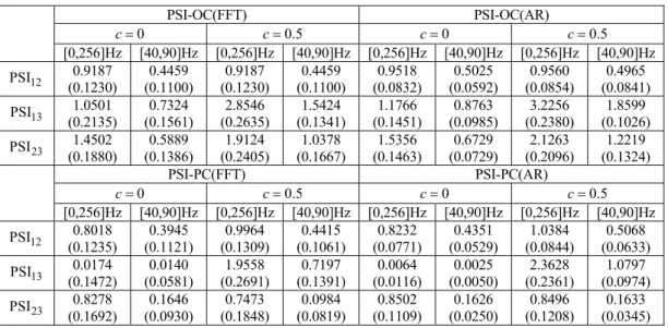
x and x₂ (Eq. (19)), obtained by FFT and AR modelling. Table 2 – Results on PSI on two different bands. The first line is the mean, the second line in parentheses is the std.

PSI-OC(FFT) PSI-OC(AR) 0 = c 0.5c= c=0 0.5c= [0,256]Hz [40,90]Hz [0,256]Hz [40,90]Hz [0,256]Hz [40,90]Hz [0,256]Hz [40,90]Hz 12 PSI 0.9187 (0.1230) 0.4459 (0.1100) 0.9187 (0.1230) 0.4459 (0.1100) 0.9518 (0.0832) 0.5025 (0.0592) 0.9560 (0.0854) 0.4965 (0.0841) 13 PSI 1.0501 (0.2135) 0.7324 (0.1561) 2.8546 (0.2635) 1.5424 (0.1341) 1.1766 (0.1451) 0.8763 (0.0985) 3.2256 (0.2380) 1.8599 (0.1026) 23 PSI 1.4502 (0.1880) 0.5889 (0.1386) 1.9124 (0.2405) 1.0378 (0.1667) 1.5356 (0.1463) 0.6729 (0.0729) 2.1263 (0.2096) 1.2219 (0.1324) PSI-PC(FFT) PSI-PC(AR) 0 = c 0.5c= c=0 0.5c= [0,256]Hz [40,90]Hz [0,256]Hz [40,90]Hz [0,256]Hz [40,90]Hz [0,256]Hz [40,90]Hz 12 PSI 0.8018 (0.1235) 0.3945 (0.1121) 0.9964 (0.1309) 0.4415 (0.1061) 0.8232 (0.0771) 0.4351 (0.0529) 1.0384 (0.0844) 0.5068 (0.0633) 13 PSI 0.0174 (0.1472) 0.0140 (0.0581) 1.9558 (0.2691) 0.7197 (0.1391) 0.0064 (0.0116) 0.0025 (0.0050) 2.3628 (0.2361) 1.0797 (0.0974) 23 PSI 0.8278 (0.1692) 0.1646 (0.0930) 0.7473 (0.1848) 0.0984 (0.0819) 0.8502 (0.1109) 0.1626 (0.0250) 0.8496 (0.1208) 0.1633 (0.0345) When using FFT, spectra are obtained using a sliding window of

64-point length and a 50% overlap. As for AR modelling, it is real-ized on the whole signal length. For one time delay between two signals (for example, in Eq. (19), from x₁ to x₂), the theoretical value of the variation of the phase spectrum is π on the whole fre-quency band. In the upper panel of Figure 3, the variation of OC(AR) is actually close to π. For OC(FFT), some fluctuations appear in the low and high frequency bands. Since coherence ampli-tude is not unity on the whole frequency band, PSI is smaller than π for one time delay. Moreover, in the frequency band [40, 90]Hz, around 65 Hz, the slope of the coherence phase (OC(FFT) and OC(AR)) is more regular than outside this band. Consequently, hereafter, the four measures OC(FFT), PC(FFT), PSI-OC(AR) and PSI-PC(AR) are computed in the whole frequency band [0, 256]Hz and in the frequency band [40, 90]Hz. As previ-ously, we generate a set of 100 realizations of 1024 data points each. Means and standard deviations (std) are computed and shown in Table 2.

First of all, if we compare Tables 1 and 2, PSI-OC takes into con-sideration the importance of the delay contrary to LGCI: for exam-ple, PSI -OC PSI -OC₂₃ > ₁₂ whereas

2 3 1 2

LGCIx_→x <LGCIx_→x ,

for 0c= . The latter inequality does not respect the pecking order. Secondly, we can analyze the results given in Table 2 according to the three following points:

• PSI-OC versus PSI-PC

Both PSI-OC and PSI-PC perfectly point out the flow direction of information among the 3 signals. PSI-PC reveals the direct relations and distinguishes the two patterns shown in Figure 1.a and 1.b while

PSI-OC cannot distinguish them, whatever the frequency band and the computation mode (FFT or AR).

• FFT versus AR model

The results obtained with AR modelling are preferred since (i) the mean values are generally higher with AR modelling (except for the case x₁→x₃ and c=0, where PSI-PC(AR) remains closer to the theoretical null value than PSI-PC(FFT)), and (ii) the corresponding standard deviations are smaller.

• Whole frequency band versus [40, 90]Hz band

As expected, values of PSI computed on the limited band are lower than those computed in the whole frequency band. On the other hand, considering the limited band allows to reveal the pecking order of the time delays in the phase slope indicator. As for the standard deviations, they are comparable in both situations.

3.2 Nonlinear signals and linear couplings

For this study on nonlinear stochastic systems, we start from the example given in [6]: ( ) ( )

(

( )

)

( ) ( ) ( ) ( )

(

( )

)

( ) ( ) ( ) ( ) ( )

(

( )

)

( ) ( ) ( ) ( ) 2 1 2 ₁ 1 1 1 1 2 ₁ 2 ₂ 2 2 2 1 2 2 ₁ 2 3 3 3 3 2 1 3 3.4 1 1 1 3.4 1 1 1 0.5 1 (20) 3.4 1 1 1 0.3 1 1 x t x t x t x t x t x t e w t x t x t x t e x t w t x t x t x t e x t cx t w t − − − − − − ⎧ _{= − − − +} ⎪ ⎪ ⎪⎪ _{= − − − + − +} ⎨ ⎪ ⎪ _{= − − − + − + − +} ⎪ ⎪⎩

where 0c= and c=0.5 are chosen to examine the same patterns of causal interactions as in Figure 1. Noises w t_j

( )

,j=1, 2,3, are

independent white Gaussian processes, with zero means and vari-ances equal to 0.04. We simulated Eq. (20) to generate a data set of 100 realizations of 1024 time points each.

3.2.1. Results on LGCI

Since we already demonstrated that LGCI-M outperforms LGCI-P, we only present results on LGCI-M. Means and standard deviations are reported in Table 3.

Table 3 – Results on LGCI-M. The first line is the mean, the sec-ond line in parentheses is the std. Reciprocal indices tend to zero.

LGCI-M 0 = c 0.5c= 1 2 LGCI_x→x 0.2248 (0.0283) 0.2310 (0.0241) 1 3 LGCI_x→x 0.0003 (0.0013) 0.2289 (0.0287) 2 3 LGCI_{x →x} 0.1053 (0.0208) 0.1022 (0.0192)

From this table, it is clear that LGCI-M can point out the direct causality and distinguish the two patterns of causal interactions in the nonlinear stochastic system.

3.2.2. Results on PSI

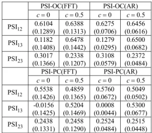
Since there is no dominant frequency in these nonlinear signals, the PSI is only estimated on the whole frequency band. Means and standard deviations are shown in Table 4.

Table 4 – Results on PSI. The first line is the mean, the second line in parentheses is the std. PSI-OC(FFT) PSI-OC(AR) 0 = c 0.5c= c=0 0.5c= 12 PSI 0.6104 (0.1289) 0.6388 (0.1313) 0.6275 (0.0706) 0.6456 (0.0616) 13 PSI 0.1182 (0.1408) 0.6478 (0.1442) 0.1279 (0.0295) 0.6500 (0.0682) 23 PSI 0.3017 (0.1366) 0.2338 (0.1207) 0.3108 (0.0579) 0.2372 (0.0484) PSI-PC(FFT) PSI-PC(AR) 0 = c 0.5c= c=0 0.5c= 12 PSI 0.5538 (0.1426) 0.4859 (0.1365) 0.5760 (0.0672) 0.5049 (0.0502) 13 PSI -0.0156 (0.1425) 0.5204 (0.1469) 0.0008 (0.0044) 0.5300 (0.0677) 23 PSI 0.2438 (0.1331) 0.2458 (0.1290) 0.2524 (0.0484) 0.2515 (0.0448) After analyzing the results in Table 4, we come to the conclusion that (i) OC(FFT), PC(FFT), OC(AR) and PSI-PC(AR) identify carefully the flow direction of information in this nonlinear stochastic system, (ii) PSI-PC(FFT) and PSI-PC(AR) can reveal the direct relations and distinguish between patterns. PSI-OC(AR) and PSI-PC(AR) are more relevant than PSI-OC(FFT) and PSI-PC(FFT), mainly in terms of standard deviation.

4.

CONCLUSIONS

In this paper, we focused on information propagation between multi-site observations using a phase slope index based approach. The technique proposed relies on (i) the introduction of partial coherence instead of ordinary coherence to deal with causal rela-tions, (ii) AR modelling to reduce estimator variance. Combining both improvements allow to distinguish direct and indirect causal

relations in linear and non linear time series with the lowest error. Compared to Granger causality index, the new index takes into account the importance of the delay. In a next work, we plan to test it on real neurobiological time series.

5.

ACKNOWLEDGEMENTS

This work was supported by China Scholarship Council (CSC) un-der Grant No. 2008609145.

REFERENCES

[1] N. Wiener, The theory of prediction. New York, 1956.

[2] C. W. J. Granger, "Investigating causal relations by econometric models and cross-spectral methods," Econometrica, vol. 37, pp.

424-438, Aug. 1969.

[3] J. Geweke, "Measurement of linear dependence and feedback between multiple time series," Journal of the American Statistical

Association, vol. 77, pp. 304-313, 1982.

[4] J. F. Geweke, "Measures of conditional linear dependence and feedback between time series," Journal of the American Statistical Association, vol. 79, pp. 907-915, 1984.

[5] K. J. Blinowska, R. Kuś and M. Kamiński, "Granger causality and information flow in multivariate processes," Physical Review E Statistical Nonlinear, vol. 70, pp. 050902(R), 2004.

[6] Y. Chen, G. Rangarajan, J. Feng and M. Ding, "Analyzing mul-tiple nonlinear time series with extended Granger causality," Phys-ics Letters A, vol. 324, pp. 26-35, 2004.

[7] Y. Chen, S. L. Bressler and M. Ding, "Frequency decomposition of conditional Granger causality and application to multivariate neural field potential data," Journal of neuroscience methods, vol. 150, pp. 228-237, 2006.

[8] X. Wang, Y. Chen, S. L. Bressler and M. Ding, "Granger causal-ity between multiple interdependent neurobiological time series: Blockwise versus pairwise methods," International journal of

neu-ral systems, vol. 17, pp. 71-78, 2007.

[9] W. Hesse, E. Möller, M. Arnold and B. Schack, "The use of time-variant EEG Granger causality for inspecting directed interde-pendencies of neural assemblies," Journal of Neuroscience

Meth-ods, vol. 124, pp. 27-44, 2003.

[10] M. Ding, Y. Chen and S. L. Bressler, ''Granger causality: basic theory and application to neuroscience,'' In Handbook of Time Se-ries Analysis, B. Schelter. M. Winterhalder, and J. Timmer.

Wiley-VCH: Berlin. pp. 437-460, Aug. 2006.

[11] E. Wolf, "New theory of partial coherence in the space-frequency domain. Part I: spectra and cross spectra of steady-state sources," J. Opt. Soc. Am, vol. 72, pp. 343-351, 1982.

[12] J. S. Bendat and A. G. Piersol, "Decomposition of wave forces into linear and non-linear components," Journal of Sound Vibration,

vol. 106, pp. 391-408, 1986.

[13] B. Schelter, M. Winterhalder, M. Eichler, M. Peifer, B. Hell-wig, B. Guschlbauer, C. H. Lücking, R. Dahlhaus and J. Timmer, "Testing for directed influences among neural signals using partial directed coherence," Journal of neuroscience methods, vol. 152, pp. 210-219, 2006.

[14] E. Möller, B. Schack, M. Arnold and H. Witte, "Instantaneous multivariate EEG coherence analysis by means of adaptive high-dimensional autoregressive models," Journal of neuroscience

meth-ods, vol. 105, pp. 143-158, 2001.

[15] G. Nolte, O. Bai, L. Wheaton, Z. Mari, S. Vorbach and M. Hallett, "Identifying true brain interaction from EEG data using the imaginary part of coherency," Clinical Neurophysiology, vol. 115, pp. 2292-2307, 2004.

[16] G. Nolte, A. Ziehe, V. V. Nikulin, A. Schlögl, N. Krämer, T. Brismar and K. R. Müller, "Robustly estimating the flow direction of information in complex physical systems," Physical Review