DESIGN AND ANALYSIS OF A MICROMECHANICAL
TUNING FORK GYROSCOPE
by
David W. King B.S. Mechanical Engineering,
(1987) Lehigh University
SUBMITTED TO THE DEPARTMENT OF AERONAUTICS AND ASTRONAUTICS IN PARTIAL FULFILLMENT OF THE REQUIREMENTS FOR THE DEGREE OF
MASTER OF SCIENCE IN
AERONAUTICS AND ASTRONAUTICS at the
© MASSACHUSETTS INSTITUTE OF TECHNOLOGY
May, 1989
Signature of Author
Department of A06nautics and Astronautics
"%'y, 1989
Approved by
/
Burton Boxenhorn
wr -,4 ,..I .rvisor, CSDLrroiessor waiter M. Hollister
a The.si.s Supervisor Certified by
Accepted by
-_ .,,,aL Jiiu nuwIsu i.
wachman
S•...h.. DepartmentalGGrduate Committee.in,
MASS.&ii• 1'•E. ir INSTITUTE Ac Irv rulmnlAUt_% yr IE~Ini7tJLUU;I
JUli 0,
-9
'1989
UBRARIS CI--DESIGN AND ANALYSIS OF A MICROMECHANICAL TUNING FORK GYROSCOPE by
David W. King
Submitted to the Department of Aeronautics and Astronautics on May 12, 1989 in partial fulfillment of the requirements for the degree of Master of Science in
Aeronautics and Astronautics ABSTRACT
This thesis investigates the feasibility of a micromechanical tuning fork as an angular rate sensor. The gyroscopic effect of a tuning fork, which is caused by the oscillating mass moment of inertia due to the vibrating tines, is described and demonstrated by a simple model. The gyroscopic response to an input rate about the longitudinal axis between the tines is described by a second order, linear periodic (LP) differential equation which is derived by Hamilton's variational method. If the periodic terms in the equation of motion are neglected, the gyroscopic output is shown to be oscillatory in phase with the vibrating tines and linearly related to the input rate, the system quality factor, and the mechanical gain of the gyroscope. The mechanical gain is the ratio of the oscillating component of the mass moment of inertia about the input axis to the nominal component.
The periodic terms in the equation of motion are not negligable for a lightly damped, high frequency micromechanical system. A sufficient condition for stability of the LP system is derived from the properties of the Mathieu Equation. The stability condition is specified in terms of the product of the system quality factor and the mechanical gain, and it is checked by applying Floquet Theory. The response of the gyroscopically forced LP equation is solved numerically and also estimated by a Fourier Series solution. Both of these solutions correspond with the estimated linear response within the stability region.
Mathematical models are derived for the electrostatic driving force between the two fork tines, the variable capacitance sensing of the gyroscopic rotation, the stiffness properties of the structure, and the air damping torque. In addition, possible error sources are analyzed including cross-axis sensitivity, external forces and vibration, unbalance torques, motor-sensor coupling, amplifier noise, and Brownian Noise. The system mathematical model is implemented into a computer program and a baseline design configuration is obtained which is compatible with micromachining processes. The predicted performance of the baseline design is shown to be competitive with the double gimbal micromechanical gyroscope
currently being developed.
Thesis Supervisor: Dr. Walter M. Hollister
ACKNOWLEDGEMENTS
I wish to thank Burt Boxenhorn of the Charles Stark Draper Laboratory who is responsible for the original idea of a micromechanical tuning fork gyroscope, and who has stimulated many of the ideas presented in this paper through his pioneering work on micromechanical inertial instruments. I must also extend thanks to my advisor, Professor Hollister, who provided invaluable guidance and support throughout this project. Also, I would like to express gratitiude to my colleagues who offered assistance, with special thanks to John Connally, Doug Loose, and Norm Wereley. Finally, I am indebted to The Charles Stark Draper Laboratory for providing generous support of the Micromechanical Instruments project.
This report was prepared at the Charles Stark Draper Laboratory, Inc. under internal funding.
Publication of this report does not constitute approval by the Draper Laboratory or the sponsoring agency of the findings or conclusions contained herein.
I hereby assign my copyright of this thesis toThe Charles Stark Draper
Laboratory, Inc., Cambridge, Massachusetts.
David W. King Permission is hereby granted by The Charles Stark Draper Laboratory, Inc. to the Massachusetts Institute of Technology to reproduce any or all of this thesis.
TABLE OF CONTENTS
LIST OF SYMBOLS ... vi
INTRODUCTION...1
1 GYROSCOPE DESCRIPTION AND SYSTEM MODEL...5
1.1 Tuning Fork Gyroscopic Effect... 5
1.2 Demonstration Model... 8 1.3 Micromechanical Configuration... ... 13 2 D Y N A M IC S ... ... 16 2.1 System Model... 16 2.2 Neglected M odes... 19 2.3 Equations of M otion... 24
2.4 Simplified Output Solution... ... 27
2.5 Simplified Output Transient Response... 29
2.6 Cross Axis Terms ... 30
3 SYSTEM RESPONSE ANALYSIS... ... 33
3.1 Periodically Time-Varying System ... 33
3.2 Stability in Terms of the Mathieu Equation... . 36
3.3 Approximate Forced System Response by Harmonic Balance... 44
3.4 Numerical Solution ... ... 51
3.5 Stability in Terms of Floquet Theory... 63
4 SYSTEM MATHEMATICAL MODEL... ... 66
4.1 Motor Model ... 68
4.2 Sensor M odel ... 81
4.3 Mechanical Factors ... ... 84
4.4 Dam ping M odel... 88
4.5 Error Sources... ... 95
5 D E SIG N ... 105
5.1 Geometric Constraints ... 106
6 CONCLUSIONS ... 116
6.1 Comparison with Current Micromechanical Gyro Configuration... 118
6.2 Comparison with Previously Developed Tuning Fork Gyros... 120
6.3 Future Research ... 122
REFERENCES ... 125
LIST OF SYMBOLS
ly 10 Io kt bt Wx (Ch.2) Wz (Ch.2) ton (0 19bi ifb I Ix Iz AlzIx,
y,-
:Iz
6x'1 iy', 11z EG
L (Lt, 1) h w If , fy fz (2b) fx (2a) mf mw mp mtprincipal mass moment of inertia about sensitive axis
nominal ( non-oscillating ) component of Iy
oscillating component of Iy
rotation angle of the fork relative to its base
linear stiffness coefficient of torsional spring
linear damping coefficient of torsional system
applied angular rate about sensitive axis
applied angular rate about x-axis
applied angular rate about z-axis
motor (tines) driving frequency
natural frequency of torsional system
system frequency when
od
is tuned to on
angular velocity vector of fork base with respect to inertial space
angular velocity vector of fork with respect to its base
angular velocity vector of fork with respect to inertial space
inertia tensor
principal mass moment of inertia about x-axis
principal mass moment of inertia about z-axis
oscillating component of Iz
unit vectors corresponding to fork axes
unit vectors corresponding to fork base axes
modulus of elasticity for silicon
torsional modulus of elasticity for silicon
length of tines (y-dim)
height of tines (z-dim)
width of tines (x-dim)
length of flexures
thickness of flexures width of flexures mass of each flexure mass of each wingmass of each inertial proof mass mass of each tine
Wx, Wy, wz
Q
a,qa (t)
b (t)c (t)
d (t)G (t)
B (t)
an bn x F1 F2F
0eO
d
gVd
V
0w (z)
K (k) E (k)sn (x)
rOm rot xl x2Ci
Cd
CO
AC Cfb Rfbx,y,z dimensions of each wing, respectively system quality factor
gyroscope mechanical gain Mathieu Equation parameters
second derivative term coefficient to 2nd order LP equation first derivative term coefficient to 2nd order LP equation first order term coefficient to 2nd order LP equation forcing function term for 2nd order LP equation system plant matrix
system forcing matrix Fourier sine coefficients Fourier cosine coefficients state transition matrix
second order system state vector parallel electric flux motor force
fringing electric flux motor force total motor force
permittivity constant
nominal distance between tines
nominal distance between wing and bridge electrode differential driving voltage
voltage with respect to ground applied on each tine conformal transformation function
complete elliptic integral of first kind complete elliptic integral of second kind Jacobi's elliptic sine function
nominal distance between inertial mass center and sensitive axis nominal distance between tine center and sensitive axis
distance from sensitive axis to front edge of sensor plate distance from sensitive axis to back edge of sensor plate amount of sensor capacitance increase due to rotation amount of sensor capacitance decrease due to rotation nominal capacitance of each pair of sensor plates net change in capacitance output signal
output amplifier feedback capacitance output amplifier feedback resistance
Ex
Ox
B eout bx, by, bz 4Isia0
U00 QUQf'
Ff Fp xm AzAB
Aa
a (BW) bKe
KB K0 ass,Bass,a
K1 mx, my, mz u2 0quadsensor excitation voltage sensor excitation frequency bandwidth of output signal filter output voltage
x,y,z dimensions of strain beam slot, respectively boron-silicon misfit factor
Poisson's ratio for silicon axial prestress on flexures
maximum free stream air velocity normal to wings viscosity of air flow over wings
volumetric flow rate through sensor channel profile flow rate through sensor channel
damping force due to flow impingement damping force due to pumping effect amplitude of tine vibration at tine midpoint z-direction misalignment of proof masses amplitude of white Brownian Noise amplitude of white amplifier noise system bandwidth
dynamics constant ( 10 o)
electronics constant Boltzmann's constant capacitance constant
output standard deviation due to Brownian Noise output standard deviation due to amplifier noise sensor excitation constant
x,y,z dimensions of each proof mass, respectively ratio of tine vibration amplitude to its maximum limit output oscillation amplitude in quadrature due to unbalance
INTRODUCTION
During the past several years, rapid advancements have been made in the fields of integrated circuits and microchip processing. The efficiency and accuracy in which silicon can be etched into tiny structures with dimensions in microns has led scientists to pursue the
possibility of producing mechanical elements on the microchip level. Devices such as
accelerometers, pressure transducers, flow sensors, force transducers, electrostatic actuators, and miniature microphones have already been developed and are beginning to become
commercially available. The advantages of micromechanical elements are obvious. The small size of the devices open up areas of application previously deemed unrealistic. For example, micromechanical sensors are sought after for various biomedical purposes in which conventional sensors are ineffective due to size restrictions. Also, the semiconductor batch processing techniques applied to mechanical structures greatly reduces the cost for mass production. It has now become vital for sophisticated sensors to become available cheaper in order to keep in pace with the rapidly decreasing cost of microprocessors. The two
fundamental properties of silicon make it an excellent material for sensing instruments. Its semiconductor electrical properties allow easy integration with system electronics, and its strong mechanical properties allow micromechanical instruments to be safely operated in high impact or acceleration environments.
Following this trend, in 1983 the Charles Stark Draper Laboratory, Inc. initiated the design and development of a novel micromechanical gyroscope. This represented the first development of its kind and led to a full scale project with the final goal being a complete
three axis micromechanical inertial guidance system. It has been forecast that the system will be operated in a strapdown mode with on-chip electronics, and only consist of one square inch flatpack. The gyroscope, designed by B. Boxenhorn [1,2] is planar, etched from a silicon wafer, and uses an oscillating angular momentum vector to sense angular rate about the axis normal to the gyro plane. A vibrating outer gimbal, supported by torsional pivots,
vibrates sinusoidally driven by electrostatic torquers. The oscillating angular momentum vector, combined with the angular rate, produces a gyroscopic torque on an inner gimbal causing it to vibrate about the other planar axis at the driving frequency. The inner gimbal has a vertical bar mounted on it to add inertia to the gyroscopic element. The amplitude of the inner gimbal vibration is proportional to the applied angular rate and is sensed by
ultrasensitive variable capacitance plates. The driving and sensing of the device is done by fixing electrodes above the gimbals and applying appropriate voltages.
The gyroscope has been extensively modeled, built, and tested. On 1 September
1987, The first ever micromechanical gyroscope was shown to produce gyroscopic action.
Since that important milestone rapid improvements have been made on the device including the design of a closed loop rebalance system, improvements in fabrication techniques making possible a monolithic structure with buried electrodes, and analytical models of the noise sources. The most recent test results, operated closed loop, show a gyro sensitivity of 3.13 mV/rad/sec with a noise level equivalent to 2500 degrees per hour. The gyro is projected to achieve angular rate sensing accuracy within 10 degrees per hour upon completion of the development program. At that point the device is expected to be useful in applications such as small projectile guidance, kinetic energy weapon guidance and control, land vehicle guidance and control, flight vehicle structure control and sensor stabilization, and robotics. These applications exploit the micromechanical gyroscope's qualities not present in
conventional gyros such as small size, low cost, and ruggedness.
The idea of a vibratory gyroscope is not new. In the 1950's extensive research was performed on vibratory angular rate sensors. The most popular configuration analyzed was
that of a tuning fork, where the two fork tines are forced to vibrate aganinst each other to give an oscillating mass moment of inertia about the input axis. This, in turn, produces an
oscillating torque about the axis of the fork stem proportional to an applied angular about the same axis. The Sperry Gyroscope Company designed and produced a class of these
Gyrotron would become a high performance gyro suitable for long range navigation applications. The Gyrotron, they believed, would acquire very high accuracy through continued research on eliminating the zero rate error and further modification of the angular displacement sensing technique. A decade of research continued, but, as seen retrospectively thirty years later, the tuning fork gyro proved unsuccessful and its development was
terminated.
However, it has become desirable to investigate the potential of a tuning fork
configuration on a micromechanical level, and that is the basis of this thesis. Several factors inspired the study of an alternate configuration micromechanical gyroscope, and they are listed below:
1) An investigation of the feasibility of producing a micromechanical gyroscope with
an input axis on the same plane as the gyro. A combination of two of these gyros with the current gyro would enable three gyros on a chip to sense angular rates about all three axes.
2) A thorough analysis of the tuning fork dynamics. The previous analysis of tuning fork gyros neglects the time variant terms that appear in the equations of motion. On a micromechanical level these terms become significant since it is a
lightly damped system of high frequency. It is thus necessary to determine the effect
of these terms on the gyro response and if they lead to regions of instability and poorly behaved output.
3) A simple but adequate design of a micromechanical tuning fork gyroscope. This
would make it possible to determine the performance characteristics of the gyro including its response, mechanical properties, electrical properties, and noise levels.
4) A comparison of the open loop performance capabilities between the current configuration and a tuning fork.
5) A conclusion on whether a tuning fork gyro could be successful on a micromechanical level even though all previous development efforts failed.
The thesis begins with a description of the gyroscopic properties of a tuning fork and the micromechanical gyro model to be studied. The equations of motion for the instrument are then determined rigorously by Hamilton's variational methods. This approach to the dynamics has not been attempted in the literature and will give greater insight into the system and the various small order terms neglected in the literature [3,4,5]. The next section of the thesis analyzes the full equations of motion. Due to the time variant terms in the equations no closed form solution is possible, and approximation methods are used. First, the
homogeneous equation is transformed into Mathieu's Equation which makes it possible to approximate the system stability characteristics. The approximated stability region is then checked by Floquet theory. An approximate infinite series harmonic solution is obtained for the forced equation of motion to evaluate the various harmonic components as a function of the system parameters. The approximate system responses are reinforced by a thorough
numerical simulation of the system. The last part of the paper gives design parameters of a micromechanical tuning fork gyro and calculates a set of perfomance characteristics based on
a thorough mathematical model of the system. The design is done such that the device can be built using microfabrication techniques, the response is open loop stable with maximized sensitivity, and the identified noise levels are kept to a minimum. The thesis ends by drawing conclusions on the feasibility of a micromechanical tuning fork gyroscope as an angular rate sensor.
1 GYROSCOPE DESCRIPTION AND SYSTEM MODEL
1.1 Tuning Fork Gyroscopic Effect
The operating principles of the tuning fork gyroscope are straight forward. It is possible to explain the gyroscopic torque of the device using Newton's laws, a freshman physics background, and referring to the generic schematic of a tuning fork given in Figure
1.1. This description of the gyroscope is not adequate for analytical purposes, but it should give the reader a clear understanding of the operating principles.
The two fork tines are forced to vibrate 180 degrees out of phase with each other at the same frequency, od. The vibration causes the structure to have an oscillating mass moment of inertia about the y-axis, which is the fork axis of symmetry and will hereafter be labeled the sensitive axis. The principal inertia about this axis can then be written as the sum of a constant term and an oscillating term,
* Iy = I0 + Ilsin cot. (1.1-1)
In addition to the forced tine vibration, assume that the tuning fork has only one degree of freedom which is rotation about the torsional fork stem. The stem acts like a linear torsional * spring with stiffness kt. Further assume that the system is damped linearly, and let the
damping coefficient be labeled bt. The spring and damping act as restraining torques such that
STy = - kt - bt. (1.1-2)
Let the base of the fork be fixed to a specific object which is being rotated with respect to an inertial reference frame, such that the component of the rotation vector along the fork
sensitive axis is denoted by Q. From Newton's laws the sum of the torques about the sensitive axis equals the time rate of change of the angular momentum component such that
ITy dt (Hy
* d
Differentiating the right hand side and neglecting the 0 terms, the fork equation of motion becomes
(1+ sin odt) O+(.L +l-+ cosodt ) 6 +n2 = cos dt
where Con is the torsional natural frequency of the fork, 2 kt n , O
Y
Sensitive
SAxis
fork heel
(rigid)
torsional
stem (weal
in torsion,
in bending
Forced
Vibration
k tines
base
(fixed to
platform)
Figure 1.1
Tuning Fork Schematic
A rigorous derivation that includes an analysis of the neglected terms of Equation (1.1-4) is the basis of Chapter 2. However, this simple derivation gives insight into the physics of the tuning fork gyroscope. For instance, it is clear that the gyroscopic torque term,
comes from the oscillating angular momentum about the sensitive axis and is proportional to the magnitude of the angular rate component about the sensitive axis. It is also evident that the gyroscopic torque is oscillatory at the same frequency as the vibrating tines yet in quadrature with it. It appears that an instrument can be designed that transforms the
oscillating gyroscopic torque into an output signal. This is accomplished by measuring the magnitude of an oscillating angular displacement of a torsional spring. The measurement signal can then demodulated to determine the applied rate direction, and filtered to eliminate sensitivity to lower frequency torques.
Obviously, the tuning fork instrument has little resemblence to the conventional rotated wheel gyroscope. Conventional gyroscopes are best characterized by an angular momentum vector produced by a spinning member which tends to remain fixed in space. Conventional gyroscopes detect angular rate about a particular axis by measuring the displacement of the spinning axis relative to a gimbal axis. The magnitude of the
displacement is proportional to the applied rate about a sensitive axis. On the other hand, the tuning fork instrument has an oscillating angular momentum vector, and yields an AC signal, which has its magnitude at a specified driving frequency proportional to the applied rate about a sensitive axis. Previous papers avoided the label gyroscope in describing the
tuning fork angular rate sensor. This was meant to keep the reader from thinking of the tuning fork gyroscopic reaction as produced by some fixed angular momentum vector. In this paper, however, the label gyroscope is used to describe the micromechanical tuning fork instrument. The reason is simple. The famous French physicist Jean Bernard Foucalt coined the term from its Latin translation to view rotation. The prefix gyro thus stems from the sensed angular rate, and not the instrument's rotating member.
Throughout the years, many people have had difficulty obtaining a physical feel for the action of a conventional gyroscope. With the exception of the spinning top toy, objects with a spinning member are generally not free to be rotated. Therefore, the gyroscopic reaction is not often observed in nature. However, there are several cases in nature where an
oscillating body is rotated. For one example, consider a child playing on a swing set. The child, standing on the swing, is set in motion by a friend pushing him, which is the same as an external torque applied to a rotational system. Slowly, but surely, the swing motion will damp out and the child's ride will end. But, as discovered by many ten year old
experimentalists, if the child begins to squat up and down on the swing at the proper
frequency, the swing will remain in motion. The squatting produces a periodic variation in the system mass moment of inertia, and hence causes an oscillating torque if it is in phase with the swing oscillation. This torque is proportional to the swing's angular velocity which is analogous to the tuning fork gyroscopic torque.
1.2 Demonstration Model
Even though it is likely that many people, at one time or another, have squatted up and down to force a swing, the reader may remain unconvinced that a tuning fork can sense angular rate. This leads to the first goal in the development of a micromechanical tuning fork gyroscope: to physically demonstrate that a tuning fork can produce a measurable
displacement which is proportional to an applied angular rate. To show this, a large scale model was designed to serve the function of a classroom demonstration model . It is intended to give greater insight into the physical properties of the device.
The model is shown with dimensions in Figure 1.2. The structure may not look much like a tuning fork, but it has the same basic characteristics. The model consists of a structure closed at both ends containing only a single tine. A closed fork is preferred to an open-ended structure to provide structural integrity and symmetry. For practical purposes a single tine is not desirable since it produces an inertia function which is unsymmetric about the sensitive axis. Unsymmetry leads to unbalance torques and cross-axis sensitivity. However, the demonstration model is operated by simply exciting the tines at their
fundamental frequency. A double tine structure is not feasible since it would require an identical tuning of both tines.
For the single tine the inertia function becomes
I = (I + I) + -L sin 2ot t
2 2 (1.1-5)
where Ii1 = Imax -10 , and co = driving frequency (tine fundamental frequency).
This differs from the double tine symmetric inertia function given in Eqn. (1.1-1) for two tines. For the single tine, the gyroscopic torque will be vibratory at twice the driving frequency and proportional to half of the oscillating inertia component.
The model was fabricated using beryllium copper sheets, aluminum, bronze, and wood. The single copper tine is fixed at both ends by a sandwich joint between aluminum
blocks. Attached at the midpoint of the tine is a bronze block which acts as the high density inertial proof mass. There are two torsional flexures at each end of the device, along the
sensitive axis, made from thin rectangular copper tabs which are sandwiched into the
aluminum wings and secured to the frame. The frame is attached such that the tension in the tine, and the length of the flexures, can be easily altered. This flexibility is necessary to accurately tune the device since for any appreciable gyroscopic torsional vibration the model must be operated at resonance. This means that the torsional resonant frequency of the flexures must be twice the fundamental frequency of the tine as seen from Eqn. (1.1-5).
The model was designed such that the tine and flexures were stiff enough to hold sufficient energy to reduce damping, yet flexible enough to yield a visible frequency. The flexure torsional stiffness was assumed to follow the equation,
G 3 16 b b5
Kt = r ab [3- 3.3 6a+ 0.2 8(-) ] where,
G = torsional modulus of elasticity
L = flexure length (1.1-6)
1
1
b = 2flexure thickness
which is given by Roark and Young [7]. The fundamental frequency of the tine was determined by assuming a fixed-fixed beam, and using Dunkerley's equation [8] to accomodate the effect of the inertial mass, so that,
2 = 112 t222
)b = W1 1 2+(02 22 where,
Ol l2 +0)222
0112 = 24.7mbL3) and (0222 = 6(mL7) (1.1-7)
ob = tine fundamental frequency
l 1 = fundamental frequency of beam by itself
(022 = fundamental frequency of proof mass on a massless beam\
mb = mass of tine
mm = mass of proof mass L = tine length
Dunkerley's equation is a useful technique in analyzing structures that have known stiffness properties, yet have significant masses attached to them. The equation gives a lower bound for the beam frequency by solving the characteristic equation of the system flexibility matrix, and neglecting the higher mode components.
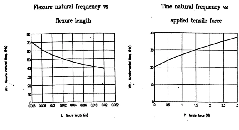
For the model, the frequencies were calculated at con = 56.3 Hz and cob = 20.1 Hz. Tuning the device such that on = 2cb was accomplished by applying tension to the tine to
push up the tine frequency while lengthening the flexures to decrease the torsional frequency, as indicated in Figure 1.3.
K~ 5*4amCa
TOP VI
EW
ID 1 0/ "lilb• ,•-4 t -. pins yS t5t CWS rtPWh 'LEWItet To wolb AV 5A ldit twj Npae(SI bE VI EW
Figure 1.2 Demonstration Model
ntr ITI V#8 Saw h""Lv" rulI**W& I [ PQres -.. . . .... .
Flexure natural frequency vs
applied tensile force
flexure length
I
L s lenth (m) P teb kfae
Figure 1.3 Resonance Tuning of Demonstration Model
Several observations were made on the model by vibrating the tine and applying an angular rate, and they are listed below:
1. The forced vibration excites a twisting mode of the tine about the sensitive axis. This mode must be of a sufficiently higher frequency than the driving
frequency since it results in an error vibration of the sensing wings.
2. The manually excited tine vibration damps out in less than five seconds due mostly to energy losses in the joint at the wing, and vibration wave
reflections back into the beam. This indicates that the device design should have no joints and a stable node where the tines are fixed to the wing. 3. Any misalignment in the z-direction of the proof masses results in an
unbalance torque about the sensitive axis. This should be minimized, yet does not provide an error since this torque is in quadrature with the
Tine natural frequency vs
gyroscope torque as shown later.
4. The thin torsional flexures, with sufficient tension applied, are very stiff in all degrees of freedom as desired.
5. The higher frequency torsional vibrations damp out slowly, mostly due to
viscous air flow.
6. Tuning the system was difficult to achieve and maintain. This indicates that the tines should be driven off resonance if possible, and a feedback loop to lock the driving frequency to the torsional resonance is desirable.
7. Gyroscopic action appeared to occur, but was difficult to verify due to tine
damping and unbalance vibrations.
1.3 Micromechanical Configuration
Although the model failed to accurately verify the gyroscopic action, it did indicate that a gyroscopic torque can be produced. The model also provided a set of useful
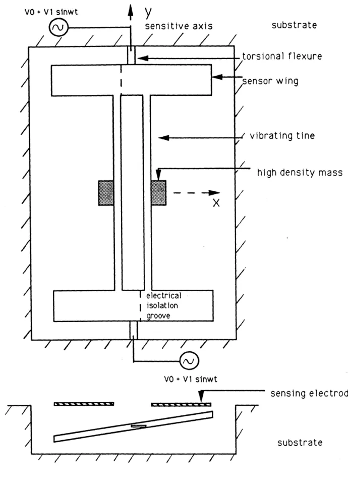
guidelines in proceeding with a micromechanical design. The most obvious requirement is that the device should have only two degrees of freedom: a forced lateral tine vibration and rotation about the torsional flexures. A simple, yet practical configuration is a double tined fork, closed at both ends, with the entire structure homogeneous and etched from a silicon chip. Attached at the midpoint of the tines is a high density metal, which serves to increase the oscillating inertia. The flexures are attached to the substrate at each end of the sensitive axis, and the entire fork is suspended over a well which allows the torsional vibration. The configuration is shown in Figure 1.5. The geometry of the configuration is simple enough that it is safe to assume that it can be fabricated by current micromachining processes such as photolithography, masking, doping, selective etching, and electroplating or metallization.
The tines will be driven electrostatically by applying a sinusiodal voltage between them. The output signal will be produced by detecting the change in capacitance between the two fork wings and electrodes either suspended above the fork , or buried in the substrate beneath it. This technique has several advantages. By keeping the driving force within the fork, coupling betweeen motor and sensor is eliminated by assuring that no motor force is transfered across the sensor gap. This coupling might represent an error source in the micromechanical gyroscope designed by Boxenhorn [1,2], and in the tuning fork gyroscope designed by Sperry [3,6]. Also, the properties of the silicon allow voltages to be applied on the tines without laying wires across the structure. This configuration also reduces damping since there are no joints, and the only air damping results from the sensor plates on the wings. Various other methods for producing a micromechanical motor have been studied in the literature [9] but electrostatics has been the most successful. The test results of the Boxenhom micromechanical gyroscope [1] demonstrate the validity of this method.
This configuration appears to offer the benefit of allowing a significant magnitude of
11
the ratio !, which is the proportional to the gyroscopic torque, while maintaining only two degrees of freedom. The subsequent chapters will provide a thorough analysis, design, and performance evaluation, based on this configuration.
VO + VI slnwt
substrate
rsional flexure
nsor wing
vibrating
tine
high density
mass
VO + V1 sinwt SI sensing electrodes
substrate
//
/
/
7/
//
/
i
/
,7~7
/
/
2 DYNAMICS
2.1 System Model
The device is modeled as a dynamic system consisting of only one degree of freedom. Figure 2.1 shows a simplified representation of the system. It contains a rigid oscillating inertia, which represents the fork structure, attached to a torsional spring. The spring is rigidly attached to a base. It might seem ambiguous that tine vibration is not considered a degree of freedom, but since its motion is constrained by the motor and its dynamics are neglected, the tine vibration is accounted in the fixed oscillating inertia term. The tine
dynamics are neglected by assuming that the driving frequency is significantly lower than the tine fundamental frequency. Also, the motor is isolated sufficiently such that it exerts no torques on the system. The only external torques acting on the system are the linear spring torque, kt0, and a viscous air damping torque, btO. The geometry is assumed to be symmetric such that any gravitational field will not result in any moment about the sensitive axis.
Three separate coordinate axes are needed to describe the system and are shown in Figure 2.1. The x-y-z coordinate system is fixed to the base of the fork which is assumed to
be strapped to a moving body. The x'-y'-z' axes are fixed to the fork. The y' axis
corresponds with the y axis, and is the sensitive axis. The x' axis runs through the center of the fork tines, and is the axis of the lateral tine vibration. The fork-based x' axis is related to the base-fixed x axis by the rotation angle, 0. The z and z' axis are defined by the right hand rule such that the z axis is normal to the substrate plane and the z' axis is normal to the fork plane. The third set of axes represents an inertial reference frame and is denoted by X-Y-Z.
Define the angular rotation of the fork base with respect to the inertial frame as the vector
Abi = Wx ix + fl y + Wzi z . (2.1-1)
The component about the y axis is denoted by 0 since it is the angular rate that the
gyroscope is designed to detect. The angular rotation vector of the fork with respect to the
fork base is,
afb = 0ly.
Then, the angular rotation of the fork with respect to the inertial frame, referenced by the
x-y-z coordinates is,
fi= fb + Wbi = Wx ix + (a + 0) iy + Wz iz. (2.1-2) The inertia of the fork is defined as a tensor referenced by the x'-y'-z' axes. These axes are chosen because they represent the principal axes for a symmetric design. Then, the inertia tensor can be written as
Ix
0 0
I = 0 Iy(t) 0
[
0
I(t)J(2.1-3)
The principal inertia components about the y' and z' axes must be written as a function of time due to the lateral vibration,
Iy (t) = 10 + Ilsin Odt , and Iz (t) = Iz + AIz sinodt, (2.1-4)
where Od designates the motor driving frequency. The fork axes and the fork base axes can be simply related by the rotation angle 0,
ix = ix' cosO + iz' sinO
iy = iyl
iz = iz' cosO -ix' sine. (2.1-5)
Substituting (2.1-5) into (2.1-2) gives the angular rotation vector in terms of the fork axes,
..i = (Wxcos0 - WzsinO) ix' + (Q + 0) iy, + (Wzcose + QsinO) iz (2.1-6)
This represents the angular rotation relative to the the fork principal axes that the device inertia is subjected to.
y,
y'
sensitive axis
oscillating inertia tensor
lateral
vibration axis
air damping torque
le
base
inertial reference frame
2.2 Neglected Modes
The single degree of freedom model of Figure 2.1 is valid only if the entire fork is rigid and free from structural vibrations. However, as observed from the demonstration model, the high frequency motor and structural unbalances excite other vibration modes. Three modes that demand concern are tine twisting, flexure bending about the x'-axis, and sensor wing bending about the sensitive axis.
The concept of rigidity is often loosely defined. In this study it will be assumed that if the free vibration frequency for a specific structural mode is significantly higher than the motor frequency, the mode will remain unperturbed. Significantly higher is generally meant meant to mean more than a factor offour larger so that the dynamic load factor [7] from the motor is approximately unity.
It is now the intention to show that for preliminary micromechanical design dimensions the three aforementioned modes can be neglected. The modes are analyzed individually as follows:
Tine Twisting: The tine is modeled as a vertical beam fixed at both ends, constrained from warping, and excited by an unbalance moment, T. The moment is applied about the tine longitudinal axis which is parallel to the sensitive axis. Figure 2.2 shows the model, and the torsional spring constant for the tine is given by Roark and Young [7] as
0.3 G h w3
k = Lt . (2.2-1)
The geometric dimensions are given in the figure. The free vibration frequency is then ,
where It is the inertia of a single tine and the attached proof mass about its longitudinal axis. The preliminary design dimensions yield the approximation,
1
It = 1o.
The driving frequency is assumed to be set at the torsional resonance of the flexures which can be determined from the stiffness Eqn. (1.1-6). Substituting, and comparing the twisting
frequency to four times the driving frequency,
0.9 G hw 3 > 16 5.3 Ga b3
Lt o L10 Io (2.2-2)
which is valid provided,
h w3 80 a b3
Lt Lf(2.2-3)
A suitable design, where the tine twisting is negligable, is when w > 5 b.
Flexure Bending : Each flexure is modeled as a beam fixed at the substrate end and subject to an excitation moment about the wing end. Assuming a Bernoulli -Euler model which neglects shear deformation and rotational inertia [9], the free vibration equation is
4
Apdu(y, t) + EI u(y, = 0
y4 (2.2-4)
where
A = cross sectional area of the beam I = beam inertia about its neutral axis
p = density of the beam material u (y,t ) = deflection curve of the beam
A solution of the form u ( y, t) = u ( y ) ei t is assumed, and fixed end - free end
boundary conditions are applied. The lowest eigenvalue solution to the transcendental vibration equation [9] is,
0o2 = 12.4 E If
f4 p Af (2.2-5)
where the subscripted terms denot the beam inertia, length and cross sectional are of the flexure. Make the approximation E 2G, substitute If = ~ (2a) (2b)3 , and compare to four times the driving frequency as given by (2.2-2) yields,
1 40.4
m-f2 -.- (2.2-6)
mfLf2 10
This statement is generally satisfied since the mass of the flexures are an insignificant portion of the structure mass.
Wing Bending: Each sensor wing is assumed to be fixed down its centerline, along the sensitive axis, at its attachment to the flexure. The angular rotation, or the tine vibration, could excite a bending moment about the y-axis, as shown in Figure 2.2. Again, using a
Bernoulli -Euler beam model with fixed end -free end boundary conditions, the
fundamental frequency is given by Eqn. (2.2-5). To correspond with the notation used for the flexure bending, let the wing dimensions be denoted by
Lw = distance from sensitive axis to end of wing
aw = one-half of wing width
bw = one-half of wing thickness mw = mass of the wing.
Comparing the fundamental wing bending frequency to four times the driving frequency results in,
2.1 aw bw2 40.4 a b3 Lw3 mw Lf 10
To approximate, assume the dimensions are such that mwL =- Io and Lw = 5Lf.
3 Then, the constraint becomes
aw b3 2 20 a b3 (2.2-8)
which is achievable for a wing thickness considerably greater than the flexure thickness(2.2-8)
O4 L 7
Flexure Bending
A
T
-em, G
t
Tine Twisting
f% ~ " v , %rhAWing Bending
Neglected Modes
SZ
u(y,t) y u(xt)z
! _ Jl • i |z
Figure 2.2
2.3 Equations of Motion
A simple, direct approach to the system dynamics was undertaken in chapter 1 resulting in the equation of motion given by Eqn. (1.1-4). In the process, several
approximations were made and the analysis was only one-dimensional. In order to account for the cross-axis terms, Hamilton's variational approach to the system dynamics is
performed which gives a more rigorous, indirect derivation of the equations of motion. Hamilton's method uses an energy technique to determine the equations that the system variables, or state vector, must obey so that the system remains at equilibrium with the external forces and constraints. Hamilton derived a variational indicator which measures the magnitude of deviation from equilibrium due to incremental changes in the state variables. The variational indicator is represented as an integral over the trajectory time period for a sum of system work increments due to the variable deviations. The equations of motion are obtained by setting the variational indicator to zero for arbitrary admissable state variations. Joseph-Louis Lagrange derived a general equation [10] for a system that obeys Hamilton's principle, and which bears his name,
T
~~-
T
-av
a4 j j (2.3-1)
for
j
= 1...n where, n = the number of state variables, and T = system kinetic coenergy4j = generalized coordinate for each state variable V = system potential energy
'j = sum of all nonservative forces in the 4j dimension. The reader is referred to Crandall et al [10] for a complete description of Hamilton's variational methods.
From the single degree of freedom system model illustrated in Figure 2.1, the only generalized coordinate is 41 = 0. The only nonconservative force acting on the system is the
linear damping, so that Zl = btL. The kinetic coenergy is due to the angular rotation of the fork ,
1
T = .fi IL fi. O (2.3-2)
It should be noted that the system kinetec coenergy is equal to the kinetic energy since the system is defined in a Newtonian reference frame. Substituting for the inertia tensor Eqn. (2.1-3) and the angular rotation vector of Eqn. (2.1-6) gives,
T = • x +,(xcos-Wsin) I Y (t) (Q+ 2
+1
Iz (t) (Wcose+Wxsine) 2The torsional spring restraining force is the only source of potential energy, so that,
V = kt 02 2
For the system, Lagrange's Equation (2.3-1) takes the form,
d DT I _-- aT aVu-+ --- = •0 where,
d
--I
T= ly (t + I) and,aeT
9dt
- = ly(t) + +l) and,_T=
-Ix
Wxcos- Wzsin0Wzcos+Wxsin
+ Izt •WFos+W xsin
W xcos_-W sine)
(2.3-4) Putting it all together, Lagrange's Equation becomes,
Iy(t) (6+0+ ly(t) (+0) +Ix ( WxcosOWzsin0X Wxsin0+Wzcose)
-Iz(t) (WzcosO+WsinOX w.cosO-wsino) + k
19
+bto
= 0.
(2.3-5)
The trigonometric terms in (2.3-5) can be expanded in a Taylor series to transform the equation of motion into algebraic form. To simplify the expansion it can be noted that the rotation angle, 0, is very small. For example, the rotation angle is on the order of 10-5 radians for the Boxenhorn gyroscope [1,2], so that first order approximations will result in negligable errors. Letting sine0 0, cos0 = 1, and sin20 = 0, and also substituting (2.1-4)
for the oscillating inertia functions, the equation of motion becomes
(lo + isindit+) IodcOSd+e) 1+ +
(wx-
I -Iz(t))0 +'kt +bte = WxWz(Ix -Iz(t))(2.3-6)
This second order differential equation represents the complete description of the tuning fork gyroscope subject to an angular rate vector. In the literature on tuning fork gyroscopes, only Fearnside and Briggs [5] included the cross-axis and small order terms in the dynamics analysis. However, the analysis done by Fearnside and Briggs differs from this paper in a few respects. Fearnside and Briggs assume the damping is of large magnitude, which is not the case on a micromechanical level. They are then able to neglect second order
Il Od
terms of the ratio . This reduces the significance of the time-varying terms present for
a lightly damped system which is studied in chapter 3. They also use a direct approach to the dynamics and simply drop all cross-axis terms after noting that they limit the device accuracy.
The first simplification made on Eqn. (2.3-6) is to neglect the angular acceleration term, Q. The driving frequency is assumed to be high enough such that the frequency of the input rate is negligable in comparison. It is then possible to drop the 0 term from the equation of motion. It must be noted that a limitation is placed on the system bandwidth, but the limitation is insignificant for practical applications. The driving frequency for a
equation of motion. It must be noted that a limitation is placed on the system bandwidth, but
the limitation is insignificant for practical applications. The driving frequency for a
micromechanical device is assumed to be in the 1-5 kHz range, and applications in guidance
or control areas do not require bandwidths greater than 100 Hz. The input frequency is thus
negligable compared to the output frequency, and no significant error results from dropping
the f term. The equation of motion can now be written in a more convenient form,
(1o
+ I1 sin odt) 0 -{ bt + I1 Od COS Odt) 0 + kt0 = -I1Z Od COS odt+( Ix - I~o
WWz
-
(W2
w
-
)
0 - III WxWz +( W
2x- W•) 0] sin
Codt(2.3-7)
2.4 Simplified Output Solution
A closed form solution to Eqn.(2.3-7) is not apparent. The first step to understanding
the behavior of the system is to drop all terms that complicate the equation and can be
reasoned to have minimal effect on the solution. The cross-axis terms on the right hand side
of the equation will be dropped first. These terms comprise a torque about the sensitive axis
that is much smaller than the spring restraining torque, the damping torque, and the
gyroscopic torque. The following section will give a more thorough analysis of the
cross-axis effects. The equation can now be transformed to a solvable form if I1 is considered
much smaller than 10, and Ilw is much smaller than bt. The equation is then a second order,
constant coefficient, harmonically forced oscillator,
Io0
0
+ b+k = -I1 0cd
COS Od t. (2.4-1)Assume a solution of the form,
0 = A sin odt
+
B cos odt,
substituting gives,
A = -I 0,2 bt
-Io( kt -lo a) + kt ( kt -lo w ) + w2 b2 and,
B = kt- Io o . (2.4-2)
The rotation angle can be maximized if the driving frequency is set at the torsional natural frequency such that,
Md = o (2.4-3)
Hereafter in this paper, when the frequency is denoted by the symbol o without a subscript, it denotes the driving frequency tuned to the torsional resonant frequency. The output is then
a pure sine curve, in phase with the motor vibration,
8
(t) = sin ot .bt (2.4-4)
The linear damping coefficient can be written in terms of the system quality factor,
Q
,I00
where bt =
-p
. A more convenient expression for the simplified output solution is-IQ Q
0
(t) = sin aot. (2.4-5)I0(
If all the assumptions for the simplified solution are valid, the output angle is
proportional to the ratio of the oscillating inertia component to the nominal inertia component, the system quality factor, the magnitude of the applied rate, and inversely proportional to the driving frequency. This gives a calibrated measure of the angular rate about the sensitive axis. The output signal can also be demodulated with the driving oscillation as a reference
2.5 Simplified Output Transient Response
Eqn. (2.4-5) gives the steady state vibration of the harmonically forced, linear
system. However, the second order dynamics of the tuning fork will lead to an oscillating
transient period that must be investigated in terms of system bandwidth. Eqn. (2.4-1) can be
written in the following form,
** * 2 - I COd
- n e -+ " + n -- COS O d t .
Q
+
0(2.5-1)
Let II (t)
=
I1 sin Odt, then Eqn. (2.5-1) can be written,
0
*•2
-i (t)
Q0
+
o
10
Since this equation is linear, Laplace transforming yields,
- I1 s - 0 - G (s) . S s2
+
ýS + Cn2 Q (2.5-2)G(s) represents the system transfer function, but it can not identify the system bandwidth since it relates the input signal which has unknown frequency to an output signal oscillating at the driving frequency. In order to transform G(s) into a DC transfer function, Gm(s), the output signal is frequency modulated at the driving frequency. This means,
0m
(t) =
8 (t)
e
1 Odor, in the Laplace domain,
Om
(s)
=(s +j
COd)Replace s by s + j wd to give the DC transfer function,
-I --- s + j Cd ) m o = Gm (s) .
Q
(s + j Od)2 + -(S + j (0d)+5 Q (2.5-3)Expanding, rationalizing, and setting the driving frequency at the resonant frequency,
s +j0)[s s+
2jws+
Gm (s)4
(os
+
f2(S
+S2
+
_.Q2
4c 2s
+2•
1
Q+
(2.5-4)
Assuming that the system bandwith is much lower than the driving frequency , the components of the transfer function can be written,
I{
s
(s
+
Imag (Gm (s)) = and , 4oýs + Q)2 -Ii Real.(Gm (s)) = I21s +
2(
Q
(2.5-5)
It is clear that the quadrature component is small compared to the in-phase component so that the signal has negligable phase shift during the transient period, and the sytem bandwidth is
BW = - . (2.5-6)
2Q
2.6 Cross Axis Terms
The right hand side of Eqn. (2.3-7) consists of the gyroscopic torque term plus four terms due to the input rate about the axes orthogonal to the sensitive axis. These terms lead to torques about the sensitive axis of unknown magnitude. But, if these torques can be shown to either have negligable effect on the system, or cause an output deflection that has no component that is in-phase with the motor at the driving frequency, no error signal will result. This is because appropriate signal filtering and demodulation can eliminate all signals from the sensor rotation except the vibrational component in phase with the motor within a
component that is in-phase with the motor at the driving frequency, no error signal will result. This is because appropriate signal filtering and demodulation can eliminate all signals from the sensor rotation except the vibrational component in phase with the motor within a small frequency band about wd. However, any quadrature or off-frequency signal must not exceed the designed output range of the gyroscope.
The cross axis terms are analyzed term by term:
1) (Ix -IOz)(WxWz) : This causes a DC output which can be filtered out. The bias that it
causes can be made as small as possible by designing the nominal inertias about the x and z axes to correspond. It appears from Figure 1.5 that the symmetry can be easily obtained by adjusting the x and y dimensions of the proof masses.
2) (Ix -Iz)(Wx 2 - Wz2) 0: For a symmetric design where Ix = I0z, this term can be regarded as a small deviation in the spring constant. But, assuming a driving frequency in
the 2-4 kHz range, and a practical limit on the cross axis rates of around 20 Hz, then kt = 62 10 >> (Ix - I0z)(Wx2 -Wz2). Hence, this term will have less than a 0.01% deviation on the spring constant and will not alter the output significantly.
3) AlzWxWz sin or : AIz is the oscillation inertia about the z-axis, and is thus small and
on the order of Ii. Again, for a high frequency system, this term is tiny compared to the gyroscopic torque for any significant Q. It is also in quadrature with the gyroscopic torque, so even for very small values of 9, the majority of the error signal from this term will be eliminated by demodulation.
4) Alz(Wx2 - Wz2) 0 sin ox : This term can be viewed as a high frequency deviation in the spring constant. Since Ilz is generally on the order of 1% of Ioz, the maximum deiviation in the spring constant from this term is only about 0.0001%. And the frequency component of
the term does not lead to difficulties since, when combined with the sinusoidal output, it results in a double frequency torque.
In general, the cross axis terms do not lead to a significant limit on the accuracy of the device. As shown in the subsequent chapters, for a micromechanical device, Brownian and electronics noise are the predominant error sources. Zero rate errors, such as cross-axis coupling, tend to be insignificant by comparison.
3 SYSTEM RESPONSE ANALYSIS
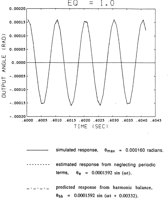
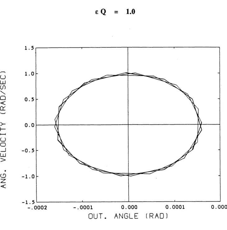
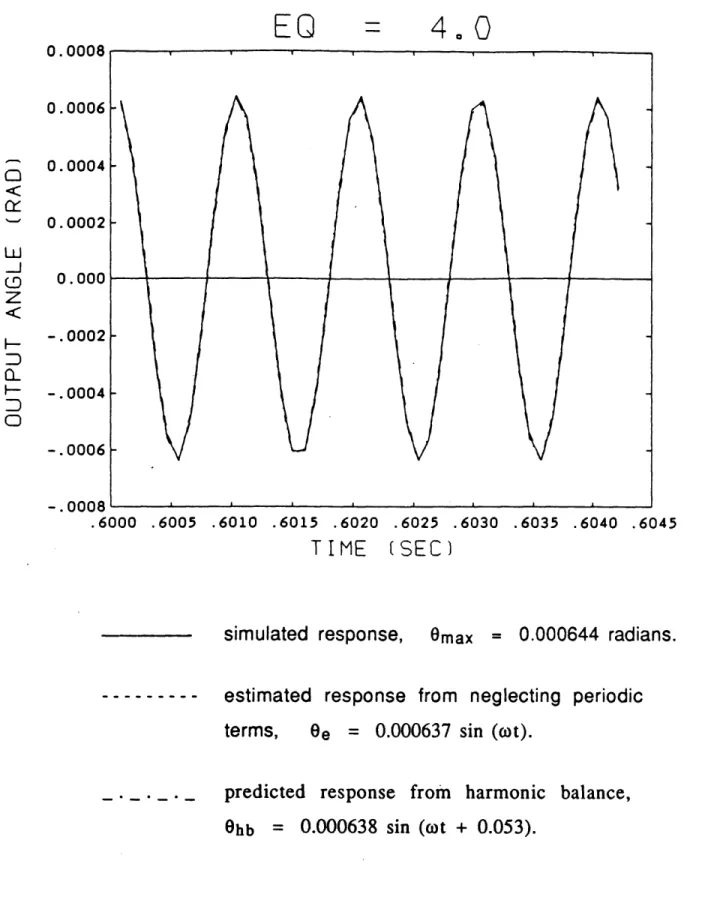
In this chapter, the system response to the complete equation of motion will be studied. For the tuning fork to operate efficiently as an angular rate sensor, the output angle must be a linear function of the input rate. Eqn. (2.4-5) shows a linear relationship, but in its derivation the periodic terms in the equation of motion were neglected. It is necessary to verify that the periodic terms have a negligable effect on the system response. A brief
overview of linear periodic equations is presented, and then the tuning fork equation of motion is analyzed by several different analytical and numerical tools.
3.1 Periodically Time -Varying System
If the cross axis terms are neglected and the system is driven at its torsional resonance so that on = COd = 0o, the complete equation of motion (2.3-7) becomes,
1 + sin)t + cos + 02 8 - 1 0 Cos ct or,
\ Io .Io Io
(1 + esin ox 0 + +e )cos 0x + 0 0 =- Q )cos 0t .
where
e = the mechanical gain
Q = sytem quality factor.
Generally, the mechanical gain is a small number, and the quality factor is defined in Eqn. (2.4-5). Equation (3.1-1) is a linear, time varying, periodic differential equation (LP) of second order. Equations of this form have arisen in many different fields of application,
and hence many different analytical methods to describe the behavior of such systems have been studied. The problem is that there is no uniform approach, such as the Laplace
transform for linear, time-invariant, differential equations, to describe these systems. There are also no known exact solutions, which makes it necessary to treat each equation
individually by the most appropriate approximate method. The equation of motion (3.1-1) is of the form
a (t) x
+
b(t)x + c(t) x = d(t)
where a, b, and the forcing function d, are all periodic of period T = 2 x / co . The main deficiency with the simplified solution of Chapter 2 is that even though a(t) = 1 since E is small, the periodic component of b(t) cannot be accurately neglected since 1 / Q is on the same order as E for a lightly damped micromechanical system. This type of equation, with nearly constant a and c and periodic b , is a rare and unexplored form of an LP equation. Intuitively, the response to Eqn. (3.1-1) will be approximately the steady state and transient response of sections 2.4 and 2.5 for a small value of the product parameter, EQ. But when EQ grows greater than unity, and the periodic component of b(t) begins to dominate, the oscillating response will deviate from the simplified solution. This can be viewed as a periodic perturbation in the damping, so that as EQ increases the output frequency should remain constant, but the output magnitude, phase, and bandwidth will be affected.
The periodic variation in the damping is an effective energy pumping of the system. This results in a substantial increase or decrease in the amplitude of the output oscillations. A physical example ofenergy pumping from the circuit design field is presented by Richards
[11]. By periodically changing the capacitor plate distance in an LC circuit network, it is possible to pump the voltage across the capacitor, which results in a periodic damping term. When done at the proper frequency and phase, this increases the magnitude of the voltage across the capacitor. This view leads to the conclusion that for specific values of the
be globally stable. The product of the mechanical gain and the system quality factor, EQ, will thus be referred to as the stability parameter.
The stability problem of periodic systems is unique because small variations in a periodic coefficient can cause the system to lie in a region of instability, separated by regions of stability. In the tuning fork case, this means that as eQ is increased past a certain limit the response could go unstable, but a continued increase in the parameter could stabilize the system. The stability problem of periodic systems has been studied in depth, with particular emphasize by Maclachlan [12], Richards [11], and Porter [13].
An optimized design of the micromechanical tuning fork gyroscope will maximize the parameter eQ, since it is a factor in the output magnitude as shown by (2.4-5). It is thus
imperative to determine the stability characteristics of this parameter. Several techniques to determine the stability of periodic systems exist. They include transformation to the Mathieu
equation, Lyapunov stability theory, Floquet theory, and numerical simulation.
In the literature, much research has been done on homogeneous equations of the
form K +[a- 2q2 (t)]x = 0 ,
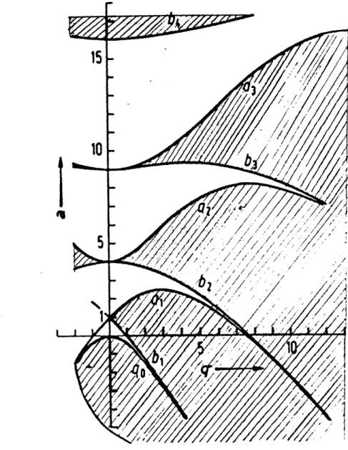
where V (t) is a periodic function. This is known as Hill's equation and has its roots date back to 1886. A special case of Hill's equation that has received particular attention in regard to stability is the Mathieu equation, and is given by
x
+ [a - 2qcos2t]x = 0 . (3.1-2)Approximate periodic solutions to Eqn. (3.1-2) have been obtained as a function of the parameters a, q. Since the stability regions for the parameters have been well documented
[11,12], a useful technique to determine the stability of a particular LP system is to transform it to the Mathieu equation. Then the characteristics of the transformed equation, plus the particular transformation, yield information about the original equation. The disadvantage of this approach is that an appropriate transformation must be found, and information can be lost in the transformation.
Another approach is based on Floquet theory. This is recently emerging as a useful technique to give an exact yes or no answer to a particular system stability. However, this approach is limited in that it requires the computation of a discrete transition matrix, and its respective eigenvalues, for a given set of parameters. For the majority of LP systems, the discrete transition matrix cannot be obtained in closed form. Numerical techniques must be used and the stability conclusions are only obtained for specific values of the parameters.
Lyapunov stability theory, a more theoretical approach, uses mathematical functional analysis to check if a suitable bound can be determined for the system response. It has been used successfully for many particular periodic equations, but it requires the formulation of a suitable Lyapunov function. There is no defined method to determine the Lyapunov
function, and extensive trial and error is often the method employed. Unfortunately, the Lyapunov function is not easily obtained for the tuning fork equation.
The last possible technique, numerical simulation, has the problems of truncation and round-off error, and is very sensitive to errors around the stability limits. Also, the high frequency oscillations in an unstable region can grow slowly over many periods, so extensive computation time is needed to reach conclusions. Simulation, though, can be used to
reinforce analytical results and verify the forced system response.
3.2 Stability in Terms of the Mathieu Equation
In order to transform Eqn. (3.1-1) into a form of the Mathieu equation of (3.1-2), it is first written in a more convenient form. Dividing through by the a(t) term and noting the first order expansion
1
= 1 - E sin ot + O (E2) (3.2-1)
gives,
0 + + cos ax) 1 - e sin ) 0 + 2 1 - esin oca = -E co (I - esinct) Cos ct. Again, neglecting the second order terms in e, gives
O
+ o+ E coos ot - Qsin wt i + 2 ( - esinwt)O = -eocosxt.If, for a lightly damped system, the parameter i is on the order of e, then the sine component of the b(t) term is negligable compared to the cosine component. This gives
0 + ( + e) cos t + 2 (1 - esinot)O =-0 e tocos a.
An appropriate change of variables must be found that eliminates the b(t) term from the homogeneous form of Eqn. (3.2-2). An appropriate transformation [11] is
x = 0exp- -
b(')
x=Bnp(2 ",
d) (3.2-3) which transforms the equation0 + b(t) 0 + c(t) 0 = 0 x + [c(t) 1.- . (t) into 1 b2(t)]x = 0.
-4
x0
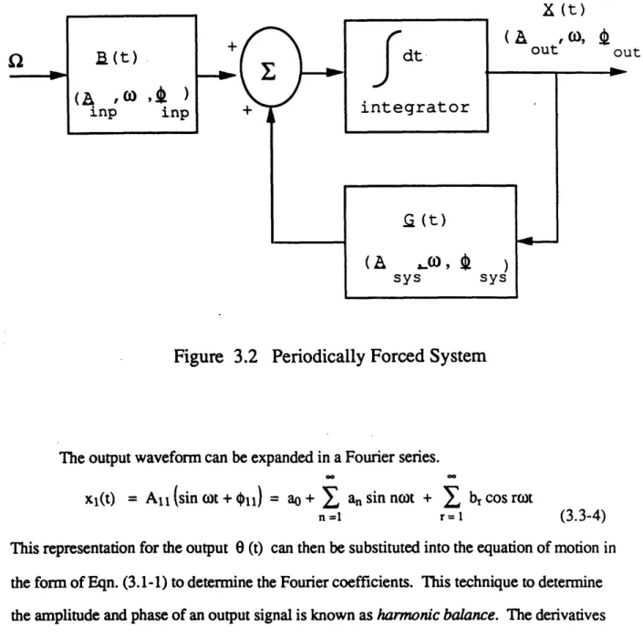
(3.2-4) Substituting the values for a(t) and b(t) from Eqn. (3.2-2) yields the transformed equation,S + t2 1 4 •-) --F.sin (°t -1- cos -2t COS2•t x = 0.
4
Q2
2 2 Q 4 (3.2-5)The oscillating component of the second term of Eqn. (3.2-5) is approximated by the sine component since Q >> 1 and e << 1. The transformed equation is then written