• Aucun résultat trouvé

The CuSum algorithm - a small review

N/A
N/A
Protected

Academic year: 2021

Partager "The CuSum algorithm - a small review"

Copied!
23
0
0

Texte intégral

(1)

HAL Id: hal-00914697

https://hal.archives-ouvertes.fr/hal-00914697

Submitted on 13 Mar 2014

HAL is a multi-disciplinary open access

archive for the deposit and dissemination of

sci-entific research documents, whether they are

pub-lished or not. The documents may come from

teaching and research institutions in France or

L’archive ouverte pluridisciplinaire HAL, est

destinée au dépôt et à la diffusion de documents

scientifiques de niveau recherche, publiés ou non,

émanant des établissements d’enseignement et de

recherche français ou étrangers, des laboratoires

The CuSum algorithm - a small review

Pierre Granjon

To cite this version:

(2)

The CUSUM algorithm

a small review

Pierre Granjon

GIPSA-lab

March 13, 2014

(3)

Contents

1 The CUSUM algorithm 2

1.1 Algorithm . . . 2

1.1.1 The problem . . . 2

1.1.2 The different steps . . . 3

1.1.3 The whole algorithm . . . 5

1.1.4 Example. . . 7

1.2 Performance. . . 7

1.2.1 Criteria . . . 7

1.2.2 Optimality . . . 9

1.3 Practical considerations . . . 9

1.3.1 Dealing with unknowns . . . 9

1.3.2 Setting the parameters. . . 12

1.3.3 Two-sided algorithm . . . 15

1.4 Variations . . . 18

1.4.1 Fast initial response CUSUM . . . 18

1.4.2 Combined Shewhart-CUSUM . . . 19

1.4.3 Multivariate CUSUM . . . 19

(4)

Chapter 1

The CUSUM algorithm

Lai [Lai 1995] and Basseville [Basseville 1993] give a full treatment of the field, from the simplest to more complicated sequential detection procedures (from Shewhart control charts [Shewhart 1931] to GLR algorithm first given in [Lorden 1971]).

1.1

Algorithm

It is Page who first proposes different forms of the cumulative sum (CUSUM) algorithm in [Page 1954a]:

• direct or recursive forms. • one- or two-sided forms,

1.1.1

The problem

Let X[n] be a discrete random signal with independent and identically dis-tributed samples. Each of them follows a probability density function (PDF) p(x[n], θ) depending on a deterministic parameter θ (for example the mean µX or the variance σ2

Xof X[n]). This signal may contain one abrupt change occur-ring at the change time nc. This abrupt change is modeled by an instantaneous modification of the value of θ occurring at the change time nc. Therefore θ = θ0 before nc and θ = θ1 from nc to the current sample.

Under these assumptions, the whole PDF of the signal pXobserved between the first sample x[0] and the current one x[k] can take two different forms.

• Under the no change hypothesis (H0), the PDF of X[n] is given by: pX|H0 =

k Y n=0

(5)

• Under the one change hypothesis (H1), this PDF becomes: pX|H1 = nYc−1 n=0 p(x[n], θ0) k Y n=nc p(x[n], θ1) . (1.2)

In this problem, the PDF of each sample p (x[n], θ) and the values of the pa-rameter before (θ0) and after (θ1) the abrupt change are supposed to be known. Finally, the only unknowns to be determined are:

• the lack or occurrence of an abrupt change between n = 0 and n = k, • the value of the possible change time nc.

In order to develop the desired algorithm, we follow an on-line approach. This means that the abrupt change possibly contained in the past of the signal has to be sequentially detected sample after sample. Therefore, at each new sample x[k], one of the two previous hypotheses H0 and H1 has first to be decided. Then, in the case a change has been detected (H1decided), the change time has to be estimated thanks to an estimatorcnc. The general form of this sequential algorithm is given in algorithm1.

initialization if necessary end

while the algorithm is not stopped do measure the current sample x[k]

decide between H0 (no change) and H1 (one change) if H1 decided then

store the detection time nd← k estimate the change time nc stop or reset the algorithm end

end

Algorithm 1: general form of a sequential change detection algorithm. Two important steps appear in this algorithm :

detection step: How to decide between H0 and H1?

estimation step: How to efficiently estimate the change time nc? These steps are further detailed in the two following sections.

1.1.2

The different steps

Detection step

The problem here is to decide between two possible hypotheses H0and H1from the measured samples x[0], . . . , x[k], which is also termed a binary hypothesis

(6)

testing problem. The solution, given by the detection theory, is to use the so-called likelihood ratio test [Kay 1998, chap. 3]:

test 1. Let the log-likelihood ratio LXbe defined by: LX= ln p X|H1 pX|H0  . (1.3)

Then, decide H1 if LX> h (else H0), where h is a threshold set by the user. In our case, the theoretical expression of LX at the current sample x[k] is ob-tained by reporting (1.1) and (1.2) in (1.3):

LX[k, nc] = ln p X|H1[k, nc] pX|H0[k]  = k X n=nc ln  p(x[n], θ1) p(x[n], θ0)  . (1.4)

Unfortunately, this quantity can not be calculated since it depends on the un-known change time nc. Once again, the detection theory leads to an efficient solution which consists of replacing all the unknowns in LX by their maximum likelihood estimates. Such a test is termed the generalized likelihood ratio test, and is given by [Kay 1998, chap. 6]:

test 2. Let the generalized log-likelihood ratio GX be defined by: GX[k] = max 1≤nc≤k LX[k, nc] = max 1≤nc≤k k X n=nc ln  p(x[n], θ1) p(x[n], θ0)  . (1.5)

Then, decide H1if GX[k] > h (else H0), where h is a threshold set by the user. The quantity defined in (1.5) can now be calculated at each new sample and is thus used to decide between H0 and H1. It is also termed a decision function. Estimation step

Once H1 has been decided and an abrupt change has been detected, the prob-lem is to efficiently estimate the change time nc from the measured samples x[0], . . . , x[k]. One way to solve this problem is to use its maximum

likeli-hood estimate, which is the value of nc maximizing the likelihood pX|H1[k, nc]

[Kay 1993, chap. 7]: c nc = arg max 1≤nc≤k pX|H1[k, nc] = arg max 1≤nc≤k LX[k, nc] = arg max 1≤nc≤k k X n=nc ln  p(x[n], θ1) p(x[n], θ0)  . (1.6)

(7)

1.1.3

The whole algorithm

Direct form

In order to obtain a simplified form of the whole algorithm, let’s define from (1.4) the instantaneous log-likelihood ratio at time n by:

s[n] = LX[n, n] = ln  p(x[n], θ1) p(x[n], θ0)  , (1.7)

and its cumulative sum from 0 to k: S[k] =

k X n=0

s[n]. (1.8)

From (1.7) and (1.8), the log-likelihood ratio LX[k, nc] defined in (1.4) can be rewritten as:

LX[k, nc] = S[k] − S[nc− 1]. (1.9) Reporting this expression in (1.5) and (1.6), we obtain new expressions for the decision function GX[k] and for the change time estimatencc[k]:

GX[k] = S[k] − min 1≤nc≤k S[nc− 1] (1.10) c nc = arg min 1≤nc≤k S[nc− 1]. (1.11)

Equation (1.10) shows that the decision function GX[k] is the current value of the cumulative sum S[k] minus its current minimum value. Equation (1.11) shows that the change time estimate is the time following the current minimum of the cumulative sum. Therefore, each step composing the whole algorithm relies on the same quantity: the cumulative sum S[k] defined through (1.7) and (1.8). This explains the name of cumulative sum or CUSUM algorithm. By using equations (1.7), (1.8), (1.10) and (1.11) into algorithm 1, the direct form of the CUSUM algorithm2is obtained.

Recursive form

The previous algorithm can easily be rewritten in a recursive manner. Indeed, the cumulative sum (1.8) can be calculated through the simple recursive formula:

S[k] = S[k − 1] + s[k]. (1.12)

Moreover, as shown in [Basseville 1993, chap. 2], since the decision function is compared to a positive threshold h, it can be rewritten as:

GX[k] = {GX[k − 1] + s[k]}+, (1.13) where {z}+= sup(z, 0). Finally, by using (1.12) and (1.13) into the direct form algorithm2, the recursive form of the CUSUM algorithm3is obtained. Clearly, the obtained algorithm is very simple and very interesting to use in real-time or on-line applications.

(8)

initialization

set the detection threshold h > 0 k= 0

end

while the algorithm is not stopped do measure the current sample x[k] s[k] = lnp(x[k],θ1) p(x[k],θ0)  S[k] =Pkn=0s[n] GX[k] = S[k] − min1≤nc≤kS[nc− 1] if GX[k] > h then nd← k c nc= arg min1≤nc≤kS[nc− 1]

stop or reset the algorithm end

k= k + 1 end

Algorithm 2: CUSUM algorithm, direct form.

initialization

set the detection threshold h > 0 S[−1] = GX[−1] = 0

k= 0 end

while the algorithm is not stopped do measure the current sample x[k] s[k] = lnp(x[k],θ1) p(x[k],θ0)  S[k] = S[k − 1] + s[k] GX[k] = {GX[k − 1] + s[k]}+ if GX[k] > h > 0 then nd← k c nc= arg min1≤nc≤kS[nc− 1]

stop or reset the algorithm end

k= k + 1 end

(9)

1.1.4

Example

Let us consider the particular case where the signal X[n] is constituted of inde-pendent and identically distributed samples following a Gaussian distribution with mean value µXand variance σX2. This signal is supposed to undergo a pos-sible change in the mean at a change time nc. The changing parameter θ is then µX, which takes the values µX 0 before and µX 1 after the change. Therefore, the theoretical expression of the PDF followed by each sample is:

p x[n], µX j= 1 σX √ 2πe −(x[n]−µXj) 2 2σ2X , where j = 0 before and j = 1 after the change.

A particular realization x[n] of X[n] is represented on top of Fig.1.1with µX 0 = 0, µX 1 = 1, σX2 = 1 and nc = 1000. It is clear from this curve that a simple threshold applied to x[n] is insufficient to efficiently detect the presence of an abrupt change and estimate the change time nc.

The CUSUM algorithm is applied to this signal by using its recursive form

3, and a detection threshold set to h = 100. The values of µX 0, µX 1 and σ2

X are supposed to be known, contrarily to nc. Therefore, the instantaneous log-likelihood ratio s[n] can be calculated whatever the time n through the expression: s[n] = µX 1− µX 0 σ2 X  x[n] −µX 1+ µX 0 2  . (1.14)

Fig.1.1shows the typical behaviour of this algorithm. As expected, the decision function GX[n] stays close to 0 before and grows continuously after the change time. The presence of the change is detected when GX[n] > h at nd = 1201 (see the red line), leading to a detection delay of nd− nc = 201 samples. Once the change has been detected, the time following the current minimum of the cumulative sum S[n] gives the estimated change timecnc= 1001. Consequently, the estimation error of the change time |nc − cnc| = 1 is very small for this example.

1.2

Performance

1.2.1

Criteria

Several criteria have been proposed to measure the performance of change de-tection algorithms, but the following ones are the most popular.

Average run length function The average run length (ARL) function pro-posed in [Page 1954a] is defined as the expected number of samples before an action is taken:

(10)

0 200 400 600 800 1000 1200 −2

0 2 4

measured signal x[n] ; abrupt change at nc=1000

0 200 400 600 800 1000 1200

−2 0 2

instantaneous log−likelihood ratio s[n]

0 200 400 600 800 1000 1200 0 50 100 150 decision function Gx[n] → nd = 1201 0 200 400 600 800 1000 1200 −500 0

cumulative sum S[n] → estimated n

c = 1001

Figure 1.1: typical behaviour of the CUSUM algorithm in the case of an iid Gaussian signal with a change in the mean at time nc = 1000.

where Nd is the detection time of the change detection algorithm, and the parameter θ is assumed constant for all the signal samples. More particularly, the ARL function takes two interesting values with respect to θ:

• If θ = θ0, (1.15) becomes ARL0= Eθ0[Nd], the ARL to false alarm. This

quantity corresponds to the expected number of samples before a false alarm is signaled, and can be viewed as the average time between two false detections. Obviously, this quantity has to be as large as possible to minimize the rate of false detections.

• If θ = θ1, (1.15) becomes ARL1= Eθ1[Nd], the ARL to change detection.

In this case, it corresponds to the expected number of samples before the detection of a change, and is similar to an average detection delay. Therefore, this quantity has to be as small as possible to minimize the reaction time of the algorithm.

Worst case detection delay This criterion has been first proposed in [Lorden 1971]. Let first define the conditional expected detection delay by EH1

h

(Nd− nc+ 1)+|X[0], . . . , X[nc− 1] i

(11)

the one change hypothesis H1 (PDF given by (1.2)). A minimax performance criterion is given by its supremum taken over (nc, X[0], . . . , X[nc− 1]):

EH1[Nd] = sup nc≥0 n ess sup EH1 h (Nd− nc+ 1)+|X[0], . . . , X[nc− 1] io . (1.16) This quantity is the worst case detection delay of the change detection algorithm. It obviously has to be as small as possible in order to minimize the quickness of reaction to an abrupt change in the signal.

1.2.2

Optimality

Page uses ARL0 and ARL1in [Page 1954a] to conclude on the good the perfor-mance of the CUSUM algorithm, but gives no result about its optimality. Next, Lorden [Lorden 1971] shows the asymptotic optimality of the CUSUM algorithm with respect to the worst case detection delay. More precisely, let the detection threshold h (see algorithm2or3) be so chosen that the ARL to false alarm verifies ARL0 ≥ γ > 0. Clearly, this condition is equivalent to limit the rate of false detections by a given maximum value. When γ → ∞, the CUSUM algorithm minimizes the worst case detection delay EH1[Nd]. Moreover, the

value of this delay can then be approximated by: EH1[Nd] ∼ ln γ I (pθ0, pθ1) , (1.17) where I (pθ0, pθ1) = Eθ1 h lnp(X[n],θ1) p(X[n],θ0) i

denotes the Kullback-Leibler informa-tion number.

Later, Moustakides [Moustakides 1986] and Ritov [Ritov 1990] generalize this result to the non asymptotic case (for finite ARL0) by using non-Bayesian and Bayesian approaches.

1.3

Practical considerations

The goal of this section is to mention the main problems encountered when the CUSUM algorithm is used in practice, and provide some possible solutions.

1.3.1

Dealing with unknowns

Section 1.1 shows that the CUSUM algorithm entirely relies on the instanta-neous log-likelihood ratio s[n] defined by Eq. (1.7). This quantity depends on the probability density function of the signal samples, and thus on its different parameters. For example, the case of a change in the mean in a iid Gaussian signal studied in paragraph1.1.4 leads to Eq. (1.14), where s[n] depends on the mean values before and after the change µX 0 and µX 1 and on the variance σ2

X. Until now, all these parameters were supposed known, which is a quite unrealistic assumption for practical applications. In the case where different

(12)

parameters are unknown, the online evaluation of s[n] becomes impossible and the CUSUM algorithm cannot be employed.

To overcome this problem, the optimal method consists of using the generalized likelihood ratio test principle by replacing in s[n] all the unknown parameters by their maximum likelihood estimates. This leads to the generalized likelihood ratio or GLR algorithm initially presented in [Lorden 1971]. Unfortunately, this optimal algorithm cannot be written in a recursive manner and its com-plexity grows with the number of available samples, contrarily to the CUSUM algorithm. This explains that the GLR algorithm cannot be used for online applications.

Another possibility is to preserve the simple and recursive structure of the CUSUM algorithm, even if this leads to suboptimal algorithms. Following this point of view, different situations may be encountered:

θ1 unknown: This is the most common practical case. Indeed, in most ap-plications the true value of the changing parameter after change is not precisely known. In that case, the usual solution is to use the classical CUSUM algorithm where θ1 is a priori set by the user, i.e. employed as an additional parameter. A logical and efficient way to set this parameter is to choose the most likely value that θ1 should take after the change. The precision of this setting clearly depends on the amount of a priori information the user has about the signal. The resulting algorithm is gen-erally suboptimal, but results of section1.2show that it is still optimal to sequentially detect changes from θ0 to the chosen value of θ1.

θ0 and/or constant parameters unknown: In that case, the situation is not as critical as the previous one and a simple solution exists. Indeed, these unknowns can be replaced by their maximum likelihood estimates using the available samples at time k, i.e. x[0], . . . , x[k]. Moreover, ef-ficient implementations can be obtained by using recursive estimators. Finally, the resulting algorithms use the generalized likelihood ratio test principle and are nearly optimal.

As an example, let’s once again consider the case studied in paragraph1.1.4of a change in the mean in an iid Gaussian signal. µX 1 is usually rewritten with respect to µX 0 as:

µX 1= µX 0+ δ, (1.18)

where δ is the change magnitude of the mean value.

By using (1.18) into (1.14), the corresponding instantaneous log-likelihood ratio then becomes: s[n] = δ σ2 X  x[n] − µX 0δ 2  . (1.19)

This relation shows that s[n] depends on the mean value before change µX 0, the constant variance of the signal σ2

Xand the change magnitude δ. If all these parameters are unknown, the two strategies described in this paragraph have to be jointly applied:

(13)

δ unknown: replace the true value of δ in (1.19) by a parameter ˜δset to the a

priori most likely change magnitude,

µX 0 and σ2

X unknown: replace the true values of µX 0 and σ2X in (1.19) by their maximum likelihood estimatesµcX 0 and cσX2 at the current sample. This finally leads to algorithm4, where two parameters have now to be a priori set: the detection threshold h and the change magnitude ˜δ.

initialization

set ˜δ to the most likely change magnitude set the detection threshold h > 0

S[−1] = GX[−1] = 0

initialize the estimatorsµcX 0 and cσ2 X k= 0

end

while the algorithm is not stopped do measure the current sample x[k]

calculate the current estimatesµcX 0[k] and cσ2 X[k] s[k] = ˜δ c σ2 X[k]  x[k] − cµX 0[k] − ˜δ 2  S[k] = S[k − 1] + s[k] GX[k] = {GX[k − 1] + s[k]}+ if GX[k] > h > 0 then nd← k c nc= arg min1≤nc≤kS[nc− 1]

stop or reset the algorithm end

k= k + 1 end

Algorithm 4: suboptimal CUSUM algorithm, jump in the mean - iid Gaus-sian case.

In order to compare optimal and suboptimal CUSUM algorithms, algorithm4

is applied to the signal previously used in section1.1.4, with the same detection threshold h = 100 and a change magnitude perfectly set to ˜δ= 1. Results, illus-trated in Fig.1.2, show that the two algorithms have the same general behavior, but a slightly more important detection delay is obtained with the suboptimal algorithm.

Finally, this methodology leads to a suboptimal algorithm having the same global complexity and behavior as its optimal version obtained in section1.1.3, and reaching almost similar performance. The main difference is that this al-gorithm necessitates the setting of one additional parameter, the change mag-nitude, thanks to a priori information the user may have concerning abrupt changes occurring in the signal.

(14)

0 200 400 600 800 1000 1200 −2

0 2 4

measured signal x[n] ; abrupt change at nc=1000

0 200 400 600 800 1000 1200

−2 0 2

instantaneous log−likelihood ratio s[n]

0 200 400 600 800 1000 1200 0 50 100 150 decision function G x[n] → nd = 1278 0 200 400 600 800 1000 1200 −400 −200 0

cumulative sum S[n] → estimated n

c = 1001

Figure 1.2: typical behaviour of the suboptimal CUSUM algorithm in the case of an iid Gaussian signal with a change in the mean at time nc= 1000.

1.3.2

Setting the parameters

The CUSUM algorithm have several tuning parameters the user has to correctly set:

• in any case the detection threshold h,

• in case of the previous suboptimal CUSUM algorithm, θ1 or equivalently the change magnitude.

the change magnitude The previous section shows that the user must have

a priori knowledge about the signal to correctly set this parameter. Indeed,

an efficient setting for the change magnitude is the a priori most likely change magnitude that should appear in the signal. In case several magnitudes of jump are possible, the best choice is the minimum one. In any case, the resulting change detection algorithm is only optimal to sequentially detect the chosen change magnitude. Notice that an a posteriori choice of the most likely change magnitude leads to the GLR algorithm [Lorden 1971].

(15)

the detection threshold The classical way to set this parameter is to use the average run length function (1.15), and more particularly the mean time between false alarms ARL0 and the mean detection delay ARL1. These two specific values of the ARL function depend on the detection threshold h, and can thus be used to set the performance of the CUSUM algorithm to a desired value for a particular application. A first possibility is to choose the mean time between false alarms to a desired value NF A:

• fix the desired mean time between false alarms NF A= ARL0(ho), • compute the corresponding optimal threshold value ho= ARL0−1(NF A), • deduce the resulting mean detection delay ARL1(ho).

Another possibility is to first choose the mean detection delay to a value ND the user desire:

• fix the desired mean detection delay ND= ARL1(ho),

• compute the corresponding optimal threshold value ho= ARL1−1(ND), • deduce the resulting mean time between false alarms ARL0(ho).

Obviously, such a method requires the knowledge of the different values of the ARL function, and several approaches has been proposed in the literature to evaluate this function in the CUSUM case [Basseville 1993, chap. 5]:

Integral equation approach: Page demonstrates in [Page 1954a] that this ARL function is the solution of an integral equation of Fredholm’s type. Un-fortunately, finding an analytical solution to this equation is generally im-possible. To overcome this problem, several methods have been proposed to numerically evaluate this solution, see for example [Goel 1971]. This first approach can lead to very accurate results, but is computationally intensive.

Approximation approach: Different analytical approximations of this ARL function relying on the theory of sequential analysis [Wald 1947] have been proposed, see for example [Page 1954b] and [Siegmund 1985]. This second approach is simpler than the previous one, but generally leads to less accurate results.

Markov chain approach: Following this approach, it is not only possible to evaluate the average run length function, but also the statistical prop-erties of the CUSUM algorithm such as the run length distribution. It has been introduced in the discrete case in [Brook 1972], adapted to the continuous case in [Lucas 1982a, Lucas 1982b], and further investigated in [Yashchin 1985a,Yashchin 1985b].

As an example, Fig. 1.3 shows Siegmund’s approximation [Siegmund 1985] of ARL0(h) and ARL1(h) in case of a change in the mean of magnitude δ = 1 in

(16)

0 0.5 1 1.5 2 2.5 3 3.5 4 0 100 200 300 400 X: 3.5 Y: 201.2 ARL 0 samples 0 0.5 1 1.5 2 2.5 3 3.5 4 0 2 4 6 8 10 X: 3.5 Y: 7.351 ARL 1 h samples

Figure 1.3: Siegmund’s approximation of ARL0(h) and ARL1(h), case of a change in the mean in an iid Gaussian signal with a SNR = δ

σX = 1.

an iid Gaussian signal of variance σ2

X= 1. This corresponds to a signal to noise ratio SNR = δ

σX = 1. Several things are highlighted by this figure. First, the

mean time between two false detections ARL0 is clearly much more important than the mean detection delay ARL1whatever the value of h. For example, the two data-tips show that the CUSUM algorithm applied to such a signal with a detection threshold h = 3.5 generates a false detection every 200 samples in mean, and detects a change in the mean of magnitude 1 with a delay of 7 samples in mean. Second, h is directly related to the algorithm reactivity or sensitivity: the smaller h, the more reactive or sensitive the algorithm. Indeed, abrupt changes are detected after very small delays for small h, but the price to pay is to obtain at the same time a small time between false detections, or equivalently a high false alarm rate. On the contrary, the same algorithm generates small false detection rates for large thresholds, but with large detection delays. The methodology explained in this section finally allows the user to set the CUSUM parameters such that this algorithm reaches desired performance in terms of mean time between false alarms ARL0and mean detection delay ARL1. Relation (1.17) can also be interesting for practical applications. Indeed, it can

(17)

be rewritten as:

ARL1∼ ln ARL0 I (pθ0, pθ1)

, when ARL0→ ∞, which roughly connects ARL1 and ARL0 when the latter is large.

1.3.3

Two-sided algorithm

Previously developed algorithms are adequate for the detection of changes in one direction only, and are called one-sided CUSUM algorithms. However, in most applications it is necessary to also detect changes in either direction. This is for example the case of a piecewise constant signal buried in noise whose changing mean must be on-line tracked.

A simple solution proposed by Page in [Page 1954a] is to use two one-sided algo-rithms, one to detect an increase and one to detect a decrease in the parameter θ. This leads to two different instantaneous log-likelihood ratios, si[n] dedicated to the increase θ0 → θi1 and sd[n] to the decrease θ0 → θd1 with θ1d < θ0 < θ1i. Two cumulative sums Si

X[n], SXd[n] and two decision functions GiX[n], GdX[n] can then be computed, and a change in the parameter is finally detected thanks to the following test:

test 3. Decide H1 if GiX[k] > h > 0  ∪ Gd X[k] > h > 0  (else H0), where h is

a threshold set by the user.

Once again, the classical way to quantify the performance of this algorithm is the ARL function. As explained in [Basseville 1993, chap. 5], the ARL function of the two-sided CUSUM algorithm can be computed from the ARL functions of the two one-sided CUSUM algorithms it is constituted. Under general conditions, these three ARL functions verify the relation:

1 ARL ≤ 1 ARLi + 1 ARLd, (1.20) where:

• ARL is related to the two-sided CUSUM algorithm,

• ARLiis related to the one-sided CUSUM algorithm corresponding to the change θ0→ θ1i,

• ARLdis related to the one-sided CUSUM algorithm corresponding to the change θ0→ θ1d.

Finally, inequality (1.20) becomes a simple equality in the case of a change in the mean of an iid Gaussian signal, and the ARL function of the two-sided CUSUM algorithm can be in this case efficiently approximated thanks to methods given in the previous section.

(18)

Applied to the case of a change in the mean in an iid Gaussian signal, this general principle leads to the two following instantaneous log-likelihood ratios:

si[n] = +|δ| σ2X  x[n] − µX 0|δ| 2  sd[n] = −|δ| σ2 X  x[n] − µX 0+|δ|2 

where |δ| is the absolute value of the change magnitude. The resulting algorithm corresponds to the well known cumulative sum control chart widely used in continuous inspection for quality control (see for example [Montgomery 2010]). Moreover, jointly applying the ideas developed in the previous section concern-ing unknown parameters leads to algorithm5. This simple and efficient recursive algorithm is able to sequentially detect increasing or decreasing changes in the mean of an iid Gaussian signal thanks to only two parameters:

• the change magnitude ˜δ, set to the most likely magnitude of change by using a priori knowledge about the signal,

• the detection threshold h, set by specifying the desired performance through the algorithm ARL function.

Fig. 1.4 shows different results obtained thanks to algorithm 5 applied to a random signal with abrupt changes. The signal of interest is an iid Gaussian signal with a constant standard deviation σ = 1 and a piecewise constant mean with three abrupt changes. The most difficult change to detect is situated at sample 800 and has a magnitude δmin= 0.5, which is smaller than the standard deviation. In Fig. 1.4, the original piecewise constant mean is represented in black and its noisy versions are represented in blue. Algorithm 5 is applied to the noisy signal with two different settings. As mentioned previously, the change magnitude parameter ˜δmust be set to the minimum change magnitude δmin = 0.5, but the mean time between false detections ARL0 can be chosen differently:

• First, ARL0= 1000. This value is a little bit too small since the last part of the signal has no change in the mean during more than 1000 samples. Therefore, the algorithm should be too much sensitive and false detections are expected in this case.

• ARL0= 2000. This value seems to be correct since the maximum number of samples between two changes in the signal is less than 2000. However, the resulting algorithm should be less sensitive than in the previous case, with higher detection delays.

The red curves of Fig.1.4 represent the piecewise constant signal estimated by algorithm5and the black crosses “+” denote the corresponding detection times. Fig.1.4(a)(resp. 1.4(b)) shows the results obtained with the most (resp. less) sensitive setting. It can first be noticed that whatever the settings, all changes

(19)

initialization

set ˜δ to the most likely change magnitude set the detection threshold h > 0

Si[−1] = Gi

X[−1] = Sd[−1] = GdX[−1] = 0 initialize the estimatorsµcX 0 and cσ2

X k= 0

end

while the algorithm is not stopped do measure the current sample x[k]

calculate the current estimatesµcX 0[k] and cσX2[k] si[k] = c|˜δ| σ2 X[k]  x[k] − cµX 0[k] − |˜δ|2  sd[k] = − |˜δ| c σ2 X[k]  x[k] − cµX 0[k] +|˜δ|2 Si[k] = Si[k − 1] + si[k] ; Sd[k] = Sd[k − 1] + sd[k] Gi X[k] =  Gi X[k − 1] + si[k] ; Gd X[k] =  Gd X[k − 1] + sd[k] if Gi X[k] > h > 0  ∪ Gd X[k] > h > 0  then nd← k if Gi X[k] > h > 0  then c nc= arg min1≤nc≤kS i[n c− 1] end if Gd X[k] > h > 0  then c nc= arg min1≤nc≤kS d[n c− 1] end

stop or reset the algorithm end

k= k + 1 end

Algorithm 5: suboptimal twosided CUSUM algorithm, jump in the mean -iid Gaussian case.

(20)

0 500 1000 1500 2000 −4 −2 0 2 4

Original signal ( δmin = 0.5 ; σ = 1 )

noisy piecewise constant 0 500 1000 1500 2000 −4 −2 0 2 4

CUSUM results ( ARL0 = 1000 → h = 4.96 )

samples

noisy signal fitted signal detection time

(a) Setting: ˜δ= 0.5 ; ARL0= 1000.

0 500 1000 1500 2000 −4 −2 0 2 4

Original signal ( δmin = 0.5 ; σ = 1 )

noisy piecewise constant 0 500 1000 1500 2000 −4 −2 0 2 4

CUSUM results ( ARL0 = 2000 → h = 5.65 )

samples

noisy signal fitted signal detection time

(b) Setting: ˜δ= 0.5 ; ARL0= 2000.

(21)

are correctly detected and estimated. As expected, one false detection appears around sample number 900 in Fig.1.4(a)with the most sensitive setting. This false detection disappears with the second setting of Fig.1.4(b), but the detec-tion delays are apparently more important in this case.

Of course, these indicative results should be statistically validated, but this first example correctly illustrate the good properties of algorithm5.

1.4

Variations

Variations of the classical CUSUM algorithm has also been proposed. Here are the most simple ones.

1.4.1

Fast initial response CUSUM

The classical recursive CUSUM algorithm is usually reset to zero after the de-tection of a change in the signal. The goal is here to increase its dede-tection performance and to give it a head start by changing the initial value of the cumulative sums when resetting. See [Lucas 1982b] and [Yashchin 1985a].

1.4.2

Combined Shewhart-CUSUM

The classical CUSUM algorithm is optimal to detect small persistent changes in signals, but Shewhart control charts are often faster to detect very important changes. The goal is here to combine the two algorithms in order to improve the resulting detection performance. See [Westgard 1977], [Lucas 1982a] and [Yashchin 1985b].

1.4.3

Multivariate CUSUM

The CUSUM algorithm can be easily generalized to multivariate signals. See for example [Basseville 1993, chap. 7], where the basic case of r-dimensional random vectors of Gaussian independent sequences is treated in section 7.2.1.

(22)

Bibliography

[Basseville 1993] M. Basseville et I. Nikiforov. Detection of abrupt changes: Theory and application (prentice hall information and system sciences series). Prentice Hall, 1993. 5 citations on pages2, 5,13,15, and19

[Brook 1972] D. Brook et D. A. Evans. An Approach to the Probability

Dis-tribution of the Cusum Run Length. Biometrika, vol. 59, no. 3, pages

539–549, December 1972. Cited on page13

[Goel 1971] A. L. Goel et S. M. Wu. Determination of A.R.L. and a Contour

Nomogram for Cusum Charts to Control Normal Mean. Technometrics,

vol. 13, no. 2, pages 221–230, May 1971. Cited on page13

[Kay 1993] S. Kay. Fundamentals of statistical signal processing, volume 1: Estimation theory. Prentice Hall, 1 ´edition, 1993. Cited on page4

[Kay 1998] S. Kay. Fundamentals of statistical signal processing, volume 2: Detection theory. Prentice Hall PTR, 1998. Cited on page4

[Lai 1995] T. L. Lai. Sequential Changepoint Detection in Quality-Control and

Dynamical Systems. Journal of Royal Statistical Society - Series B,

vol. 57, no. 4, pages 613–658, 1995. Cited on page2

[Lorden 1971] G. Lorden. Procedures for Reacting to a Change in Distribution. The Annals of Mathematical Statistics, vol. 42, no. 6, pages 1897–1908,

1971. 5 citations on pages2, 8,9,10, and12

[Lucas 1982a] J. M. Lucas. Combined Shewhart-CUSUM Quality Control Schemes. Journal of Quality Technology, vol. 14, no. 2, pages 51–59,

April 1982. 2 citations on pages13and19

[Lucas 1982b] J. M. Lucas et R. B. Crosier. Fast Initial Response for CUSUM Quality-Control Schemes: Give your CUSUM a Head Start. Technometrics, vol. 24, no. 3, pages 199–205, August 1982.

2 citations on pages13and18

[Montgomery 2010] D. C. Montgomery. Statistical control quality: a modern introduction (6th ed.). Wiley, 2010. Cited on page16

(23)

[Moustakides 1986] G. V. Moustakides. Optimal Stopping Times for Detecting

Changes in Distributions. The Annals of Statistics, vol. 14, no. 4, pages

1379–1387, 1986. Cited on page9

[Page 1954a] E. S. Page. Continuous Inspection Schemes. Biometrika, vol. 41, no. 1, pages 100–115, Jun. 1954. 5 citations on pages2,7,9,13, and15

[Page 1954b] E. S. Page. An improvement to Wald’s approximation for some

properties of sequential tests. Journal of Royal Statistical Society - Series

B, vol. 16, no. 1, pages 136–139, 1954. Cited on page13

[Ritov 1990] Y. Ritov. Decision Theoretic Optimality of the Cusum Proce-dure. The Annals of Statistics, vol. 18, no. 3, pages 1464–1469, 1990.

Cited on page9

[Shewhart 1931] W. A. Shewhart. Economic control of quality manufactured

product. MacMillan, London, 1931. Cited on page2

[Siegmund 1985] D. Siegmund. Sequential analysis - tests and confidence inter-vals. New York: Springer-Verlag, 1985. Cited on page13

[Wald 1947] A. Wald. Sequential analysis. New York: John Wiley and Sons,

1947. Cited on page13

[Westgard 1977] J. O. Westgard, T. Groth, T. Aronsson et C. H. De Verdier.

Combined Shewhart-cusum control chart for improved quality control in clinical chemistry. Clinicla Chemistry, vol. 23, no. 10, pages 1881–1887,

October 1977. Cited on page19

[Yashchin 1985a] E. Yashchin. On a Unified Approach to the Analysis of

Two-Sided Cumulative Sum Control Schemes with Headstarts. Advances in

Applied Probability, vol. 17, no. 3, pages 562–593, September 1985.

2 citations on pages13and18

[Yashchin 1985b] E. Yashchin. On the analysis and design of CUSUM-Shewhart

control schemes. IBM Journal Research and Development, vol. 29, no. 4,

Figure

Figure 1.1: typical behaviour of the CUSUM algorithm in the case of an iid Gaussian signal with a change in the mean at time n c = 1000.
Figure 1.2: typical behaviour of the suboptimal CUSUM algorithm in the case of an iid Gaussian signal with a change in the mean at time n c = 1000.
Figure 1.3: Siegmund’s approximation of ARL 0 (h) and ARL 1 (h), case of a change in the mean in an iid Gaussian signal with a SNR = σ δ X = 1.
Figure 1.4: Application of algorithm 5 to an iid Gaussian signal containing three 18

Références

Documents relatifs

As shown in Fig.1, firstly, the point cloud expression of the scene is constructed based on depth data, and the down sampling is performed to the point cloud by using

We used linear regressions to test how these metropolitan form metrics relate to transportation indicators that we use as proxies for sustainable metropolitan development—CO2

The ECOMORE-CNM yearly Dengue Major Outbreak Sensor, based on the Surveillance R-package is a highly performant tool to predict major incoming dengue outbreaks in Cambodia.. Its

Frequency-Dependent Peak-Over-Threshold (FDPOT) puts special em- phasis on the frequency dependence of extreme value statistics, thanks to Vector Generalized Additive Models

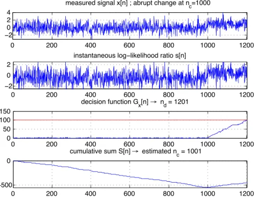
2. The rupture is detected, as the variance is proportional to the distance of the signal from its average. ! 1 length determines the noise rejection capabilities of

In particular, we shall show that the CUSUM is optimum in detecting changes in the statistics of Itô processes, in a Lorden-like sense, when the expected delay is replaced in

Spectral line removal in the LIGO Data Analysis System (LDAS). of the 7th Grav. Wave Data Anal. Coherent line removal: Filtering out harmonically related line interference

In the case of a research prototype using an imperfectly matched lens array and LCD panel, the displayed pattern may be interpolated to achieve sub-pixel alignment, with a small