Convolutional neural networks for image reconstruction and image quality assessment of 2D fetal brain MRI

Convolutional Neural Networks for Image Reconstruction and Image Quality

Assessment of 2D Fetal Brain MRI

by Sayeri Lala

S.B., Electrical Engineering and Computer Science,

Massachusetts Institute of Technology, 2017

Submitted to the

Department of Electrical Engineering and Computer Science

in Partial Fulfillment of the Requirements for the Degree of

Master of Engineering in Electrical Engineering and Computer Science

at the

Massachusetts Institute of Technology

June 7, 2019

© 2019 Massachusetts Institute of Technology. All rights reserved.

Author: ________________________________________________________________ Department of Electrical Engineering and Computer Science

May 22, 2019

Certified by: ________________________________________________________________ Elfar Adalsteinsson

Professor, Department of Electrical Engineering and Computer Science Professor, Institute for Medical Engineering and Computer Science May 22, 2019

Accepted by: ________________________________________________________________ Katrina LaCurts, Chair, Master of Engineering Thesis Committee

Convolutional Neural Networks for Image Reconstruction and Image Quality

Assessment of 2D Fetal Brain MRI

by Sayeri Lala

Submitted to the Department of Electrical Engineering and Computer Science

June 7, 2019

In Partial Fulfillment of the Requirements for the Degree of Master of Engineering

in Electrical Engineering and Computer Science

ABSTRACT

Fetal brain Magnetic Resonance Imaging (MRI) is an important tool complementing Ultrasound for diagnosing fetal brain abnormalities. However, the vulnerability of MRI to motion makes it challenging to adapt MRI for fetal imaging. The current protocol for T2-weighted fetal brain MRI uses a rapid signal acquisition scheme (single shot T2-weighted imaging) to reduce inter and intra slice motion artifacts in a stack of brain slices. However, constraints on the acquisition method compromise the image contrast quality and resolution. Also, the images are still

vulnerable to inter and intra slice motion artifacts.

Accelerating the acquisition can improve contrast but requires robust image reconstruction algorithms. We found that a Convolutional Neural Network (CNN) based reconstruction method scored significantly better than Compressed Sensing (CS) reconstruction when trained and evaluated on retrospectively accelerated fetal brain MRI datasets of 3994 slice images from 10 singleton mothers. On 8-fold accelerated data, the CNN scored 13% NRMSE, 0.93 SSIM, and PSNR of 30 dB compared to CS which scored 35% NRMSE, 0.64 SSIM, and PSNR of 20 dB. The results suggest that CNNs could be used to reconstruct high quality images from accelerated acquisitions, so that contrast quality could be improved without degrading the image.

Automatically evaluating the image quality for artifacts like motion is useful for noting what images need to be reacquired. On a novel fetal brain MRI quality dataset of 4847 images from 32 mothers with singleton pregnancies, we found that a fine-tuned Imagenet pretrained neural network scored 0.8 AUC (95% confidence interval of 0.75-0.84). Saliency maps suggest that the CNN might already focus on the brain region of interest for quality evaluation. Evaluating the quality of an image slice takes 20 ms on average, which makes it feasible to use the CNN for flagging nondiagnostic quality slice images for reacquisition during the brain scan.

Our findings suggest that CNNs can be used for rapid image reconstruction and quality assessment of fetal brain MRI. Integrating CNNs into the protocol for T2-weighted fetal brain MRI is expected to improve the diagnostic quality of the brain image.

Thesis supervisor: Elfar Adalsteinsson, Ph.D.

Title: Professor, Department of Electrical Engineering and Computer Science Professor, Institute for Medical Engineering and Science

Acknowledgments

Thank you to my thesis supervisor, Professor Elfar Adalsteinsson, for all your kind support and guidance in my research journey. I appreciate all the wisdom you shared with me. You provided a lab environment rich with opportunities and a research community that encouraged me to be brave, have confidence, and grow as a researcher. I am very grateful for all the support and kind guidance I have received from Professors Ellen Grant, Polina Golland, Jacob White, Larry Wald, and Luca Daniel. I am glad and humbled to have had the opportunity to meet and work with such bright, motivated colleagues from our labs at MIT (Magnetic Resonance Imaging Group, Medical Vision Group, Computational Prototyping group), Boston Children’s Hospital, and the Martinos Center. To name a few, thank you Yamin, Junshen, Molin, Borjan, Jeff, Filiz, Esra, Patrick, Nalini, Danielle, Ruizhi, Maz, Larry, Irene, Nick, and Daniel. I look forward to future opportunities to work together.

Thank you Megumi for your kind administrative help. Thank you to the Research Lab of Electronics Information Technology team for all the technical help.

I am also very grateful for all the research funding I received from NIH R01 EB017337 and U01 HD087211.

Thank you to my advisors at MIT: Professors Patrick Winston, Dennis Freeman, Peter Hagelstein, George Verghese, and Anantha Chandrakasan, to name a few. I am very grateful for all your invaluable mentorship since my undergraduate days.

Thank you to all my friends at MIT who have made the journey unforgettable. Dearest mom, dad, and brother Sayan: thank you for always being with me in mind and heart. You always believed in me and have always been there to give me all your strength and happiness. Everyday, you help me overcome challenges in the path to my dreams even while fighting your own battles. You are the most wonderful friends I could have ever asked for. I always love you.

Sayeri Lala MIT, 2019

Contents

1 Overview of Fetal Brain MRI 11

2 Convolutional Neural Networks for Image Reconstruction of 2D

Fe-tal Brain MRI 13

2.1 Introduction . . . 13

2.2 Background . . . 15

2.3 Methods . . . 17

2.4 Results and Discussion . . . 21

2.5 Conclusion and Future work . . . 25

3 Convolutional Neural Networks for Image Quality Assessment of 2D Fetal Brain MRI 27 3.1 Introduction . . . 27

3.2 Background . . . 30

3.3 Methods . . . 33

3.4 Results . . . 40

3.5 Discussion . . . 45

3.6 Conclusion and Future work . . . 55

3.7 Appendix . . . 57

4 Conclusion 59

List of Figures

2-1 Comparison of images from Single Shot T2W and Multi shot Turbo

Spin Echo Sequences . . . 14

2-2 Retrospective undersampling technique . . . 18

2-3 Cartesian undersampling mask . . . 18

2-4 CNN Cascade Architecture . . . 19

2-5 Normalized Root Mean Square Error for the different reconstruction approaches . . . 21

2-6 Structural Similarity Index for the different reconstruction approaches 22 2-7 Peak Signal to Noise Ratio for the different reconstruction approaches 23 2-8 Sample reconstructions for acceleration factor of 2 . . . 23

2-9 Sample reconstructions for acceleration factor of 6 . . . 24

3-1 Scan time for SST2W stacks . . . 29

3-2 Automated slice prescription engine for fetal brain MRI . . . 29

3-3 Example diagnostic quality fetal brain MRI . . . 34

3-4 Representative examples of nondiagnostic quality fetal brain MRI . . 35

3-5 Example CNN Architecture . . . 36

3-6 Dataset versions . . . 36

3-7 Example of fetal brain segmentation processing . . . 37

3-8 Examples of poor quality segmentations . . . 39

3-9 Distribution of the average slice and stack quality per subject in the dataset. . . 40 3-10 Distribution of the slice and stack quality across subjects in the dataset. 41

3-11 Representative loss curves for neural network architectures . . . 41

3-12 ROC curves for different neural network architectures . . . 43

3-13 ROC curves for different dataset versions . . . 44

3-14 Example classifications and saliency maps . . . 47

3-15 Changes in saliency map as a function of classification score . . . 48

3-16 Comparison of class activation patterns for classifiers trained on differ-ent dataset versions . . . 50

3-17 Test set artifact distribution . . . 51

3-18 Accuracy by artifact . . . 51

3-19 Distribution of the artifact source across subjects . . . 52

3-20 Example stack profiles . . . 53

3-21 Effects of class weighted loss function for neural net training . . . 54

3-22 Examples of failure modes of the segmentation approach on poor qual-ity images . . . 58

List of Tables

3.1 Original Dataset Distribution . . . 37

3.2 Brain-masked Dataset Distribution . . . 37

3.3 AUC comparison of different neural network architectures . . . 42

3.4 AUC comparison of different dataset versions . . . 42

Chapter 1

Overview of Fetal Brain MRI

Fetal brain Magnetic Resonance Imaging (MRI) is an important tool complementing Ultrasound for diagnosing fetal brain abnormalities [9, 23]. While MRI provides higher quality tissue contrast compared to Ultrasound [23, 18], it is more vulnerable to motion artifacts because data acquisition is slow relative to the dynamics of body motion, such as breathing and blood flow [49]. This makes it challenging to adapt MRI for fetal imaging since fetal motion is more random and larger compared to adults [23].

To reduce effects from motion, the current protocol for fetal brain volume MRI acquires a stack of T2-weighted (T2W) slices in a slice by slice fashion using the the single-shot T2 weighted (SST2W) imaging sequence, also known under the vendor names of HASTE, Single Shot- Fast Spin Echo, Single Shot - Turbo Spin Echo. This sequence rapidly acquires the data per slice ( 500 ms) by applying a single excita-tion pulse followed by a series of refocusing pulses. Image reconstrucexcita-tion algorithms (GRAPPA with R=2 acceleration and partial fourier) are then used to aggregate slice data from multiple receive coils to produce a slice image. Thicker slices are acquired to improve signal to noise and image the volume faster to mitigate inter slice motion artifacts [9]. Technicians often reacquire entire stacks of data in hopes of reducing motion artifacts. [4, 23]

However, the protocol is still vulnerable to inter and even intra slice motion ar-tifacts. Also, this protocol compromises quality for speed. Shorter acquisitions

com-bined with longer echo train lengths produce images with poorer T2W contrast and resolution, compared to other conventional T2W acquisition schemes (e.g., multi shot Turbo Spin Echo) [9].

These problems suggest ways in which the protocol can be improved to efficiently deliver higher diagnostic quality T2W fetal brain MRI. Better image reconstruc-tion algorithms could be developed to improve the contrast and resolureconstruc-tion quality. Prospective methods for mitigating motion artifacts are expected to improve the qual-ity of the brain volume. For example, an automated slice prescription engine (Fig. 3-2), as proposed in the fetal grant, which tracks the fetal pose to prescribe slices and monitors the quality of acquired image slices could efficiently acquire the data while mitigating inter and intra slice motion artifacts.

This thesis describes research on exploring Convolutional Neural Networks for fetal brain MRI image reconstruction and quality assessment.

Chapter 2

Convolutional Neural Networks for

Image Reconstruction of 2D Fetal

Brain MRI

2.1

Introduction

Recent work on T2W fetal brain MRI reconstruction has focused on volume super resolution and motion artifact mitigation [42, 43, 26, 17]. Improving the quality of 2d slice images would also improve the quality of the volume image.

A typical 2d slice image in fetal T2W brain imaging suffers from relatively poor in plane resolution and T2W contrast quality compared to T2W images acquired in neonate, pediatric, and adult populations (Fig. 2-1). The quality difference is due to difference in acquisition schemes used across the populations. The SST2W sequence is used for fetal brain imaging due to its relative robustness to intra scan motion artifacts. However, all data is acquired after a single excitation pulse, which results in T2 blurring, and the relatively short scan time degrades the resolution.

Techniques like the multi shot Turbo Spin Echo (TSE) sequence can be used for postnatal, pediatric, and adult brain imaging. This sequence produces images with better resolution and T2 weighted contrast [29, 30] since data is acquired over multiple

excitations and over longer scan times.

Accelerating the SST2W acquisition is expected to improve the T2W contrast and bring it closer in quality to the higher T2W contrast quality of a multi shot TSE acquired image. Other benefits from acceleration include increased safety (reduced SAR) and faster scan times, with subsequently more robustness to inter and intra slice motion artifacts. To leverage the benefits of an acceleration, this project explores image reconstruction methods for an accelerated SST2W acquisition.

(a) Single Shot T2W (b) Multi Shot Turbo Spin Echo

Figure 2-1: Figure distributed with permission from Dr. P. Ellen Grant, Director of Fetal-Neonatal Neuroimaging and Developmental Science Center Professor of Radi-ology and Pediatrics, Harvard Medical School. Figure sourced from the fetal grant. Left: Axial slice image of a fetal brain acquired with SST2W sequence. Right: Axial slice image of a neonate brain acquired with Multi shot Turbo Spin Echo sequence. The Multi shot Turbo Spin Echo acquired image has superior T2W contrast quality and resolution than the SST2W image.

The arrows point to subtle contrast differences corresponding to gray structures and heterotopic gray matter visible in the Multi shot Turbo Spin Echo image but not in the SST2W image.

2.2

Background

Image reconstruction algorithms reconstruct the MR image from the measured Fourier data, also known as the k-space. Under ideal conditions, such as sufficient sampling, magnetic field homogeneity, no patient motion, etc., one could reconstruct the MR image by applying an inverse Fourier transform to the k-space. However, these con-ditions are difficult to satisfy due to time, hardware, and physiological constraints. Image reconstruction algorithms have been developed to remove artifacts caused by k-space undersampling, scanner imperfections, or patient motion [13].

Parallel imaging reconstruction algorithms, like GRAPPA[12], SENSE [31], and ESPIRiT [44], leverage redundancies in k-space measurements from multiple phased array coils to reconstruct images from accelerated acquisitions. Parallel imaging has been adopted in various clinical applications, including fetal brain [9], pediatric body [45], and adult liver [5] MRI.

Compressed sensing (CS) has emerged as a state of art reconstruction method that exploits the inherent sparsity of MR images to remove undersampling artifacts [22]. Various CS algorithms have been developed to adapt to parallel imaging, dif-ferent sampling patterns, static vs. dynamic MRI [47]. Several studies demonstrated promising CS applications in body and liver MRI [45, 5].

Deep learning approaches have recently been explored for MR image reconstruc-tion and enhancement [25], demonstrating faster yet comparable or higher quality reconstructions compared to CS. For example, [36] trained a cascade of CNNs for reconstructing dynamic 2D cardiac MRI. On data undersampled by factors up to 11-fold, the CNN produced similar quality images in a few seconds, compared to state of the art dictionary learning CS which took several hours. [24] trained Generative Adversarial Networks for image reconstruction of undersampled abdominal MRI. On data undersampled by factors up to 10, the network produced higher quality images in 30 ms compared to compressed sensing which took 1800-2600 ms.

The current protocol for T2W fetal brain MRI uses parallel imaging (GRAPPA) with acceleration factor of 2, combined with partial fourier techniques [9]. This work

evaluates the potential of CS and deep learning based image reconstruction for further accelerating T2W fetal brain MRI.

2.3

Methods

This work investigates image reconstruction methods for accelerated SST2W acqui-sitions. The following sections describe how the dataset was prepared and the image reconstruction algorithms used in the experiments.

2.3.1

Dataset Preparation

Source

A dataset of magnitude images from vendor reconstructions of acquired k-space data was used. The data was sourced from 10 previously acquired research and clinical scans of mothers with singleton pregnancies and no pathologies, ranging in gestational age between 19-37 weeks. Scans were conducted at Boston Children’s Hospital with Institutional Review Board approval. Scans were acquired using the SST2W sequence (HASTE) with echo times of 100-120 ms, repetition times of 1.4-1.6 s, field of view between 26-33cm, isotropic in plane resolution of 1-1.3mm, and slice thickness of 2.5-3mm. The pixel resolution per image slice was 256x256.

The magnitude images served as ground truth. The retrospective undersampling scheme described below was used to generate corresponding images with undersam-pling artifacts. The acceleration factors used in this study were 2, 4, 6, and 8.

The dataset was partitioned into a training and test set, where the training set had 7 patients’ data of 2886 images and the test set had 3 patients’ data of 1108 images. The training set was used for neural network training as well as tuning regularization parameters for CS.

Retrospective Undersampling Scheme

Retrospective undersampling was used to simulate data acquired from undersampled acquisitions, as shown in Fig. 2-2. Cartesian undersampling masks were generated using the method in [36]. Fig. 2-3 shows a sample mask.

In this undersampling scheme, the phase encodes were undersampled and the fre-quency encodes were fully sampled. The target acceleration factor determined the

number of phase encodes sampled. 10 phase encodes in the central k-space were al-ways sampled. The remaining phase encodes were sampled according to a Gaussian distribution with higher probability density on lower spatial frequencies. Represen-tative example aliasing artifacts induced by this sampling scheme is shown in the zero-filled reconstruction in Fig. 2-2, where the aliasing artifacts lie along the phase encode [46].

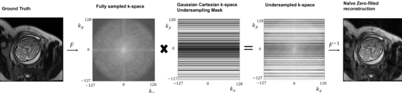
Figure 2-2: In retrospective undersampling, the fully sampled k-space of the original image is undersampled by elementwise multiplication with a k-space undersampling mask. Applying inverse fourier transform to the filled k-space yields the zero-filled image reconstruction.

Figure 2-3: A cartesian undersampling mask was used in the retrospective undersam-pling scheme. Central k-space was sampled with remaining phase encodes sampled according to a Gaussian distribution which placed higher probability over lower spa-tial frequencies.

2.3.2

Image Reconstruction Methods

Zero-filled

The zero-filled (ZF) reconstruction method is the image obtained by applying an inverse Fourier transform to the zero-filled k-space matrix, visualized in Fig. 2-2. Zero-filling the k-space matrix means that points in the k-space matrix which are not sampled are replaced with 0s.

Compressed Sensing

This study experimented with the original CS formulation in [22]. Code from [22] was used for implementation.

Daubechies wavelet was used as the sparsifying transform. The regularization parameter trading off penalties on data consistency and sparsity terms was tuned on the training dataset and optimized using the normalized root mean square error.

Deep Learning Architecture

The cascade of CNNs architecture in [36] was used.

The architecture is comprised of a series of CNNs interleaved with data consistency steps, as shown in Fig. 2-4. The input into and output of each CNN and data consistency step is an image.

Figure 2-4: Figure reproduced from [36]. The architecture is comprised of a series of CNNs interleaved with data consistency steps. The input into and output of each CNN and data consistency step is an image, with the zero-filled image as the initial input into the architecture.

set to nd = 5 and the number of cascading iterations or data consistency steps was

set to nc = 5. All convolutional layers used ReLu activation, 2d filters with kernel

size 3x3. The final convolutional layer had 2 filters to output a complex valued image while the remaining convolutional layers used 64 filters.

The data consistency step modifies the reconstruction from the preceding CNN through corrections in k-space. If the k-space point was initially sampled, the cor-responding k-space point of the reconstruction is replaced with this initial k-space measurement. Otherwise, the value of the k-space point is not changed.

The network was trained to optimize the element-wise squared loss between the original and reconstructed image. Adam optimizer parameterized by α = 10−4, β1 =

0.9, β2 = 0.999 and weight decay of 10−7 for regularization, and batch size of 10 were

used. Network weights were initialized with He initialization.

2.3.3

Evaluation

Normalized root mean squared error (NRMSE), structural similarity index (SSIM), and peak signal to noise ratio (PSNR), were used to compare the quality of the reconstructed image against the ground truth image. The scores were averaged over the test dataset.

2.4

Results and Discussion

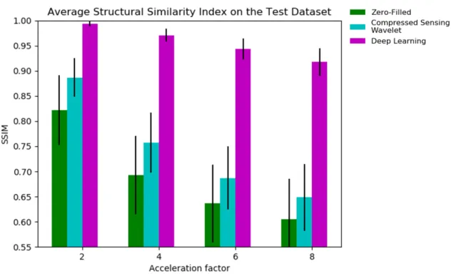
Average NRMSE, SSIM, and PSNR metrics on the test dataset are respectively shown in Fig. 2-5, 2-6, 2-7. The deep cascade CNN achieved top performance by significant margins, followed by compressed sensing, then zero-filled, as demonstrated across all metrics and acceleration factors.

Figure 2-5: Normalized Root Mean Square Error for the different reconstruction approaches. Across all acceleration factors, CNN cascade achieves significantly lower error compared to compressed sensing and zero-filled approaches. Compressed sensing performs better than zero-filled.

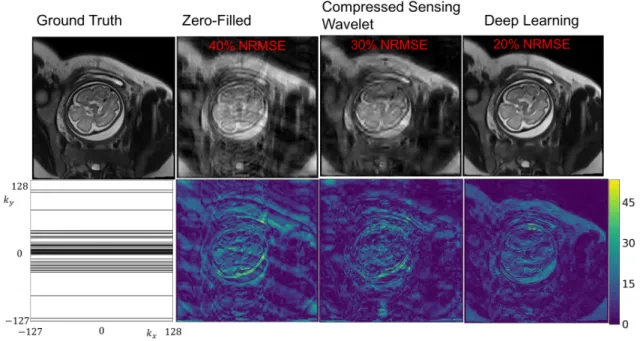
Sample reconstructions are shown in Fig. 2-8 and Fig. 2-9. ZF reconstruction is affected by severe artifacts along the phase encode axis. CS somewhat removes the artifacts but at the cost of blurring many anatomical boundaries. The CNN cascade removes undersampling artifacts and recovers anatomical features well, compared to CS and ZF reconstructions. However, the CNN also blurs some of the higher resolution features (e.g., features along the subcutaneous fat, brain boundaries like gray and white matter) and seems to affect the relative contrast differences among anatomical features (e.g., the fat and amniotic fluid appear brighter). Radiologist

Figure 2-6: Structural Similarity Index (SSIM) for the different reconstruction ap-proaches . Across all acceleration factors, CNN cascade achieves significantly higher SSIM compared to compressed sensing and zero-filled approaches. Compressed sens-ing performs better than zero-filled.

assessments indicate that the CNN reconstructions are qualitatively better than CS and ZF.

Figure 2-7: Peak signal to noise ratio (PSNR) for the different reconstruction ap-proaches. Across all acceleration factors, CNN cascade achieves significantly higher PSNR compared to compressed sensing and zero-filled approaches. Compressed sens-ing performs better than zero-filled.

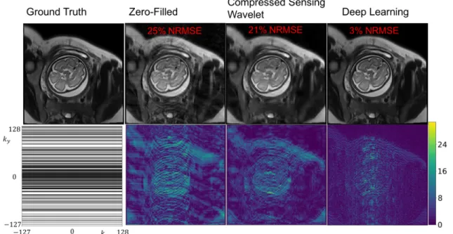
Figure 2-8: Sample reconstructions and error maps for acceleration factor of 2. Bot-tom left: k-space undersampling mask. The CNN cascade exhibits residual errors compared to compressed sensing and zero-filled approaches.

Figure 2-9: Sample reconstructions and error maps for acceleration factor of 6. The CNN cascade removes undersampling artifacts and recovers anatomical features well, compared to CS and ZF reconstructions. However, the CNN also blurs some of the higher resolution features (e.g., features along the subcutaneous fat, brain boundaries like gray and white matter) and seems to affect the relative contrast differences among anatomical features (e.g., the fat and amniotic fluid appear brighter).

2.5

Conclusion and Future work

This study demonstrates that a deep learning approach produces better reconstruc-tions compared to CS and ZF approaches and is promising method for rapidly pro-ducing high quality image reconstructions.

There are some caveats to the findings. A larger subject dataset is needed to validate the generalization and failure modes of the neural network. Also, the CS reconstructions are expected to improve upon optimizing parameters like the spar-sifying transform, parameters specific to the transform, or adding total variation penalty. Other state of the art CS techniques like dictionary learning might further improve the CS reconstructions.

Many future directions have yet to be explored. Reconstructions might be im-proved by not penalizing the network on reconstructions outside the fetal brain region of interest. Leveraging spatial correlations among neighboring slices in the volume or stack might further improve the reconstruction quality.

Towards deploying the network on prospectively sampled data, the network needs to be adapted to process complex valued measurements from multiple coils. Also, the training dataset needs to be properly generated to facilitate the network’s generaliza-tion on the prospectively sampled dataset. For example, the prospectively sampled data will have magnitude and phase and is expected to have different T2 contrast from the original SST2W vendor reconstructions. Addressing these challenges is essential for developing a deep learning based method that can be deployed on the scanner to real time reconstruct high quality T2W images.

Chapter 3

Convolutional Neural Networks for

Image Quality Assessment of 2D

Fetal Brain MRI

3.1

Introduction

The current protocol for T2-weighted fetal brain MRI attempts to prevent motion artifacts by rapidly acquiring slice data using the SST2W sequence. Due to safety constraints on the amount of exposure to radiofrequency energy, there is a 1-2s delay before imaging the next slice in the stack, so imaging a full brain stack along an orientation takes approximately 30s-1 minute as observed on sample datasets (Fig. 3-1).

The long volume scan time violates empirical guidelines of scan times < 25 seconds for ”freezing” motion [9] and is expected to suffer from inter and potentially intra slice motion artifacts. Inter slice motion manifests as misalignment of anatomies between slices. Intra slice motion artifacts can manifest as severe blurs or spin history induced non-uniform signal voids [23, 9].

Technologists try to improve the volume quality by reacquiring stacks several times [4, 23]. Fetal brain volume reconstruction techniques aim to retrospectively correct

inter slice motion artifacts via voxel wise registration and remove slices with intra slice motion artifacts via outlier detection [42, 43].

Repeated scanning makes the current protocol inefficient without guaranteeing that stacks are free of motion artifacts. Prospective methods for mitigating motion artifacts are expected to improve the acquisition efficiency and reconstruction quality of the brain volume. For example, the automated slice prescription engine (Fig. 3-2), as proposed in the fetal grant, which tracks the fetal pose to correctly prescribe the next slice in the stack, and monitor the quality of acquired slices, could mitigate inter and intra slice motion artifacts.

An automated image quality assessment (IQA) classifier that flags nondiagnostic quality slice images for reacquisition during the scan could help mitigate intra slice motion artifacts. This project is the first endeavor to develop an automated IQA classifier for low-latency detection of intra slice artifacts in fetal brain MRI.

Figure 3-1: The distribution in the scan time for an SST2W stack, analyzed on the sample dataset used in this study.

Figure 3-2: Figure distributed with permission from Dr. P. Ellen Grant, Director of Fetal-Neonatal Neuroimaging and Developmental Science Center Professor of Radi-ology and Pediatrics, Harvard Medical School. Figure sourced from the fetal grant. The automated slice prescription engine as proposed in the fetal grant. The engine tracks the fetal pose to correctly prescribe the next slice in the volume, acquires the slice, and uses an image quality assessment (IQA) classifier to real time identify nondiagnostic quality images.

3.2

Background

3.2.1

CNNs for Image Quality Assessment for MRI

Recent work [7, 40, 28, 21] has demonstrated the potential of Convolutional Neural Networks (CNNs) [16] for IQA of MRI. For example, [7] trained and evaluated a CNN for volume quality assessment of T2-weighted liver MRI on 351 and 171 cases respectively, achieving 67% and 47% sensitivities and 81% and 80% specificities with respect to 2 radiologists. [40] trained an ensemble of CNNs for volume quality as-sessment of brain MRI on pediatric and adult cases. Trained on 638 volumes and evaluated on 213 volumes, the ensemble scored 0.9 area under the Receiver Opera-tor Characteristic curve. [28] used a cohort of 3510 subjects to train and evaluate a CNN for motion artifact detection on 2D temporal cardiac MRI. The CNN scored 0.81 precision, 0.65 recall, and 0.72 F1-score. [21] finetuned and evaluated a CNN pretrained on ImageNet for quality assessment of multi-contrast carotid MRI. On a dataset of 1292 carotids drawn from 646 subjects, the CNN scored at least 67% and 74% specificity across the four image quality categories.

A couple differences exist between the problems solved in these works and the proposed problem of fetal brain MRI IQA.

These MRI quality assessment tools aim to evaluate the quality of the entire scan instead of a single slice in the scan. For example, [7, 40] evaluated CNNs for volume quality assessment. While CNNs for slice quality evaluation were trained, their performances were not reported. [28] explored motion artifact detection in cine CMR scans and investigated 3D-CNNs and Long-term Recurrent Convolutional Network to leverage temporal and spatial relationships in the 2D short axis scan data. [21] trained a CNN for detecting noise or motion artifacts in multi-contrast carotid MRI.

The artifact distribution is also different due to differences in the acquisition and imaged anatomy. In fetal MRI, motion is a dominant source of artifacts, typically ap-pearing as blurs and spin history induced nonuniform signal voids caused by in-plane

in liver, pediatric and adult brain, and cardiac imaging [8, 37], their manifestations are different. The difference is most likely due to motion in such anatomies being more regular (e.g., breathing, blood flow) and smaller in range than fetal motion [23]. Other artifacts could appear less frequently in fetal MRI, such as aliasing or field of view errors [9].

The differences in task and artifact distribution from the previous literature define this work as the first endeavor for fetal brain MRI IQA.

Given the potential of CNNs for artifact detection in MRI [7, 40, 28, 21], and their fast evaluation times on GPUs (on the order of ms), this work explores CNNs for fetal brain MRI slice quality evaluation. This study investigates transfer learning and attention mechanisms to improve CNN performance.

3.2.2

CNN methods

Scratch vs. Transfer

Transfer learning is a technique in which a neural network is initialized with the weights of a pretrained neural network and is further trained on the target dataset. Since the initial layers of deep learning models tend to learn generic image filters, transferring weights from a trained model has been demonstrated to help training models on smaller yet similar datasets compared to the source [48].

Experiments from [41] suggest that transfer learning from models trained on nat-ural images might still be useful in medical imaging applications. On tasks like polyp detection, pulmonary embolism detection, and colonoscopy frame quality assessment, they showed that finetuned CNNs compared similarly or better than the scratch CNNs, with increasing performance gains the smaller the training dataset.

Yet for IQA of cardiac MRI and pediatric and adult brain MRI, [40, 28] trained ar-chitectures using CNNs initialized from scratch and demonstrated high performance. They used large datasets derived from over 1000 subjects, which might explain the competitive performance attained using neural nets initialized with random weights. Given the different approaches in CNN weight initialization, this work studies the

impact of transfer learning for CNN training on fetal brain MRI slice IQA.

Attention Mechanisms

In fetal brain MRI, the brain occupies a small portion of the image (at most 10% of the image on a sample dataset) due to imaging parameter constraints [9]. However, the fetal brain is the region of interest (ROI) relevant for fetal brain MRI IQA, as deemed by radiologists.

Attention mechanisms that guide the neural net to focus on regions of interest have been developed for image classification and object detection [27, 10], with some performance benefit. For example, Recurrent Neural Networks were combined with reinforcement learning to discover optimal ROIs in cluttered images [27]. The algo-rithm attained 4% boost in accuracy over a CNN on a digit classification task using a cluttered MNIST dataset. The algorithm seemed to locate the digit within the image amid the clutter. For object detection, [10] used an algorithm to extract region proposals within the image, and then fed each region proposal to a CNN for feature extraction, followed by a Support Vector Machine for object classification. On the VOC 2010-12 object detection challenge, their method improved the mAP to 53% compared to a baseline with mAP of 35%.

This work experiments with the region proposal to classification approach in [10]. Unlike fetal brain MRI IQA, the problems tackled by [27, 10] involve multiple ROIs, which justify the more complex ROI search methods used in their approaches. Given the fetal brain is the ROI, the region proposal problem simplifies to segmenting the fetal brain within the image. After extracting the brain, the masked image is used for CNN training and evaluation on the IQA task.

3.3

Methods

3.3.1

Dataset Preparation

Source

A total of 7313 images were obtained from 32 previously acquired research and clinical scans of mothers with singleton pregnancies and no pathologies, ranging in gestational age between 19-37 weeks. 4847 of these images had the brain region of interest prescribed and the remaining were excluded from the dataset used in this study. Scans were conducted at Boston Children’s Hospital (BCH) with Institutional Review Board approval. Scans were acquired using the SST2W sequence (HASTE) with echo times of 100-120 ms, repetition times of 1.4-1.6 s, field of view between 26-33cm, isotropic in plane resolution of 1-1.3mm, and slice thickness of 2.5-3mm.

Labeling Criteria

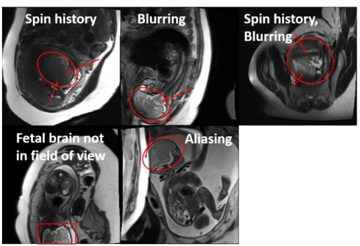
Criteria distinguishing nondiagnostic from diagnostic images was established under the guidance of radiologists at BCH. Diagnostic images were characterized by sharp brain boundaries (Figure 3-3) while nondiagnostic images were characterized by ar-tifacts that occlude such features (Figure 3-4). Motion induced arar-tifacts manifest as blurring and nonuniform signal voids over the brain region. Other artifacts manifest as aliasing or the fetus not being in the field of view. A research assistant trained under radiologists at BCH labeled the dataset.

3.3.2

CNN Experiments

Scratch vs. Transfer

VGG-16 [39] and Resnet-18 [14] architectures were adopted to assess the performance difference between neural nets trained from scratch or weights randomly initialized from a glorot uniform distribution [11], and from transfer or pretrained ImageNet model weights. All layers of the transfer neural nets were fine-tuned based on results in [48]. The input layer was modified to take in 256x256 sized images and the last fully

Figure 3-3: Example diagnostic quality fetal brain MRI

connected layer had 1 neuron for binary classification. For the transfer architectures, images were resized to 256x256x3 by replicating the image along the RGB channels. Figure 3-5 visualizes how the ImageNet pretrained VGG-16 architecture was adapted to be trained and evaluated on the dataset.

Attention Mechanisms

Following the approach in [10], the dataset was preprocessed to mask the non-brain features in images, and a neural network was trained on this masked dataset. Based on [10], several versions of the dataset (Fig. 3-6) were tried: a Brain-only, in which the non-brain features were masked out with zeros (Fig. 3-6b); and a Brain-rescaled in which the brain mask was rescaled using bilinear interpolation to fill the entire image (Fig. 3-6c). The original dataset with no masking is referred to as the Full version (Fig. 3-6a).

To compute brain masks, a neural network trained to segment fetal brains in SST2W images with similar acquisition parameters as the dataset used in this study [35] was used. Due to inaccuracies with the segmentations (Fig. 3-7a), segmentations

Figure 3-4: Representative examples of nondiagnostic quality fetal brain MRI

connected components in the segmentations, bounding circles were applied and the largest bounding circle was taken as the brain (Fig. 3-7b). After this post processing, poor quality segmentations were filtered. Noise-like segmentations were automatically filtered based on a threshold size, and remaining poor quality segmentations (Fig. 3-8) were manually filtered. Via this process, nearly 40% of segmentations on the source dataset were deemed poor quality and filtered.

Training and Evaluation Settings

The training, validation, and test set distributions for the original and brain-masked datasets are shown in Tables 3.1 and 3.2 respectively. Images were standardized to facilitate training convergence. Data augmentations were generated on the fly using translations, flips, and rotations, with parameters set to ensure that the original image quality label was preserved.

Neural networks were trained to optimize a class weighted version of the binary cross entropy loss to account for the dataset’s class imbalance [3, 6]. Stochastic gradient descent with momentum of 0.9, batch size of 50, and a properly tuned learning rate were used. The model with the lowest validation error was saved and

Figure 3-5: Adapted ImageNet pretrained VGG-16 trained and evaluated on the dataset.

(a) Full (b) Brain only (c) Brain rescaled

Figure 3-6: Different versions of the dataset used for CNN training.

used for evaluation on the test dataset.

3.3.3

Evaluation

Metrics

Receiver Operator Characteristic (ROC) curves and area under the ROC curves (AUC) were used to evaluate the classifier performance. For the top performing

(a) Inaccurate fetal brain segmentation (b) Post processed segmentation

Figure 3-7: Example of fetal brain segmentation correction

Table 3.1: Original Dataset Distribution

Dataset Partition # subjects # images % Poor quality

Training 20 3246 9

Validation 6 674 9

Test 6 927 9

Saliency Maps

Saliency maps, which aim to reveal regions within the image affecting the neural net’s decision, were applied to analyze sample classifications by the top performing model. While many saliency methods exist, Grad-CAM [38] was used since it was found to be more sensitive to the model and dataset [1].

Table 3.2: Brain-masked Dataset Distribution

Dataset Partition # subjects # images % Poor quality

Training 20 2010 6

Validation 6 505 5

3.3.4

Implementation and Code

Code and data for the experiments can be obtained from the ”cleaned” branch under the image quality assessment github repo.

The LabelBox interface was used to label slice quality. Keras with Tensorflow backend was used for training neural networks on a single NVIDIA TITAN V GPU. Saliency maps were generated using the Keras Visualization Toolkit package [15] and the ROC analysis was done using the pROC package for R [34].

Figure 3-8: Examples of poor quality segmentations (post processing) that were man-ually filtered. Segmentations were poor quality due to missing parts of the brain or including extra content outside the brain.

3.4

Results

3.4.1

Dataset analysis

Figure 3-9 shows the average distribution of non-diagnostic and diagnostic quality slices and stacks per subject. Figure 3-10 shows the distribution of non-diagnostic and diagnostic quality slices and stacks across subjects in the dataset. A stack was labeled non-diagnostic if at least 1 slice in the stack was non-diagnostic quality based on the clinical practice. Hence, while the fraction of poor quality slices is generally low, with an average 9% across subjects, this resulted in 35% stacks being non-diagnostic quality.

Figure 3-9: Distribution of the average slice and stack quality per subject in the dataset.

3.4.2

Scratch vs. Transfer

Representative loss curves shown in Figure 3-11 demonstrate that both the scratch and transfer architectures are capable of fitting the data. Table 3.3 and Figure 3-12 compare the performance of VGG-16 and Resnet-18 initialized from scratch or trans-fer settings. For the VGG and Resnet models, transtrans-fer learning scored statistically

Figure 3-10: Distribution of the slice and stack quality across subjects in the dataset.

(a) Scratch VGG-16 (b) Transfer VGG-16

Figure 3-11: Representative loss curves for neural network architectures. Model con-figurations yielding the minimum validation loss were used for evaluation.

3.4.3

Attention Mechanisms

Models using transfer VGG-16 architecture were trained independently on the Full, Brain-only, and Brain-rescaled datasets. The models scored around 0.8 AUC (Table 3.4, Figure 3-13) with no clear performance difference among the methods.

Table 3.3: AUC comparison of different neural network architectures

Architecture AUC (95% Confidence Interval) Scratch VGG-16 0.62 (0.56-0.69)

Transfer VGG-16 0.8 (0.75-0.84) Scratch Resnet-18 0.71 (0.65-0.77) Transfer Resnet-18 0.79 (0.74-0.84)

Table 3.4: AUC comparison of different dataset versions

Dataset Version AUC (95% Confidence Interval)

Full 0.78 (0.7-0.86)

Brain Only 0.83 (0.75-0.91) Brain Rescaled 0.8 (0.69-0.91)

Figure 3-12: Transfer learning improves performance over neural networks trained from scratch.

Figure 3-13: Masking non-brain features from the image has not shown any perfor-mance benefit yet.

3.5

Discussion

3.5.1

Dataset analysis

A caveat to the analysis is that nearly one third of the data comes from a pool of subjects with higher quality images than a typical subject. Hence, the fraction of the poor quality slice images and stacks is expected to increase on a larger representative dataset.

3.5.2

Scratch vs. Transfer

The performance gain from transfer learning is consistent with results in [41]. Since performance gaps tend to increase as the training set size decreases, increasing the training dataset is expected to improve the classifier.

Also, in the scratch setting, the deeper architecture Resnet-18 has statistically significant (p < 0.05) higher AUC than the shallower architecture VGG-16. Increas-ing the number of convolutional layers might help in the scratch settIncreas-ing. But, in the transfer setting, the shallower architecture VGG-16 seems to have similar per-formance as the deeper architecture Resnet-18. Decreasing or increasing the number of convolutional layers is not expected to yield any more performance gain in the transfer learning setting.

3.5.3

Attention Mechanisms

One possible reason why masking non-brain features did not boost performance is because the neural net learns to focus on the brain for classification. Figure 3-14 shows representative classifications and Grad-CAM generated saliency maps from the transfer VGG-16 model trained on the original dataset.

To validate this hypothesis, it would be ideal to quantify and compare the impact of the brain and non-brain regions of the image on the classification decision. Compar-ing the sum of class activations from the brain and non-brain regions might initially seem like a way of measuring this. However, one issue is that the class activations

are inputs to a fully connected layer and not direct inputs into the sigmoid function that outputs the class probability. Therefore, it is difficult to measure and compare the effect of the brain and non-brain regions on the classifier’s decision. Future work could explore more robust saliency map techniques that directly relate the input im-age to the classification decision. Alternatively, one could try architectures that don’t have fully connected layers, as the architectures used in the Class Activation Mapping algorithm [50].

Another hypothesis is that the classifier learns what a good quality brain looks like and if it can’t find one, labels the image as poor quality. This is consistent with observations from the saliency maps from a similar experiment as shown in Fig. 3-15. As classification score moves toward 0 or good quality, the grad-CAM activations become negative and concentrated on the brain. As the classification score moves toward 1 or bad quality, grad-CAM activations become positive and diffuse over the image.

While the classifier trained on full images might localize the brain and the regions of the brain not contaminated by artifacts, the classifier trained on brain masked datasets might better identify regions with artifacts. For example in Fig. 3-16, the neural network trained on the brain rescaled dataset better identifies the artifact and non-artifact regions in the brain. However, this does not generally seem to improve the classification.

It is possible that the small and highly skewed nature of the dataset confound the benefits of brain-masking for fetal brain MRI quality assessment. Therefore, increas-ing the dataset and reducincreas-ing the class imbalance is expected to make observations from this study more rigorous and conclusive.

3.5.4

Failure Modes

Studying the failure modes of the neural network could suggest possible techniques for improving the performance. Hence, the failure modes of the Transfer VGG-16 network trained on the original full version of the dataset were examined. Fig.

3-Figure 3-14: Example classifications and saliency maps generated by Grad-CAM. Left: Original input image. Middle: Grad-CAM results for the positive gradient weighted class activations of the image. Right: Grad-CAM results for negative gra-dient weighted class activations of the image.

classifier’s accuracy on each artifact category. To determine accuracy, the classifier’s predictions were dichotimized using a 0.5 threshold. Any prediction with score > 0.5 was labeled poor quality and was otherwise labeled good quality.

The classifier has very low performance on field of view and aliasing artifacts, compared to performance on the signal void and blurring artifacts. This is most likely due to differences in artifact representation. Analysis on the dataset shows that the signal void and blurring artifacts are better represented across subjects while the aliasing and field of view artifacts are concentrated among a few subjects (Fig. 3-19). Further, the aliasing and field of view artifacts comprise nearly 50% of the artifacts

Figure 3-15: As classification score moves toward 0 or good quality, the grad-CAM activations become negative and concentrated on the brain. As the classification score moves toward 1 or bad quality, grad-CAM activations become positive and diffuse over the image.

in the dataset given their ”streak” like nature (i.e., most of the slices in stack are affected by this artifact as shown in Fig. 3-20). This may further bias the overall classifier performance.

However, accuracy across categories is below 40%. The overall low accuracy across artifact categories yet high accuracy on diagnostic images (above 90%), is most likely due to the severe class imbalance in the dataset, with an almost 11 : 1 good to bad ratio. This observation is consistent with results in [28], where they faced a similar problem of severe class imbalance, with a 32 : 1 good to bad ratio in their cardiac image quality assessment task.

This work tried to mitigate effects from class imbalance by using a cost sensitive loss function, where the loss from a poor quality sample is weighted higher than a good quality sample to equalize the effects of each class on the CNN learning. The weights were determined according to the inverse of the class frequency. Training a CNN with a class reweighted loss function improved the AUC by about 0.05

(statis-demonstrated in Fig. 3-21.

The work in [28] reduced the performance degradation from class imbalance through data augmentation instead of using a cost sensitive loss function. They augmented their training dataset with synthesized cardiac motion artifacted data and demon-strated gains of 0.1 in precision, 0.2 in recall, and 0.06 in F1-score.

Their results suggest that classifier performance can be improved by incorporating more poor quality examples. Besides acquiring more data, synthesizing realistic fetal motion artifacts could be interesting future work. Using a physics based approach as in [28] or data generative models (e.g., Generative Adversarial Networks) might be interesting approaches for data synthesis.

Figure 3-16: Class activation patterns on a nondiagnostic image, for classifiers trained on different versions of the dataset. Top row: full, Middle row: brain only, Bottom row: brain rescaled. Left column: Original input image. Middle column: Grad-CAM results for positive gradient weighted class activations of the image. Right column: Grad-CAM results for negative gradient weighted class activations of the image. The classifier trained on the full version of the dataset identifies the non-artifact part of the brain while the other classifiers fail to do so. In particular, the classifier trained on brain only demonstrates activations in the masked regions while the classifier trained on brain rescaled demonstrates activations in only a portion of the non-artifact part of the brain. However, the classifiers trained on the brain only and brain rescaled versions of the dataset identify the artifact while the classifier trained on the full version of the dataset does not.

Figure 3-17: Distribution of the artifacts within the test set.

Figure 3-19: Distribution of the artifact source across subjects. Aliasing and field of artifacts are concentrated among a few subjects yet comprise almost 50% of the non-diagnostic quality data. Signal void and blurring artifacts are spread across subjects.

Figure 3-20: Example stack profile for a subject. Stack 28 has aliasing/field of view artifacts. These artifacts are ”streak” like, contaminating a series of slices in a single stack. Stacks 5,6, and 8 have signal void and blurring artifacts. These artifacts are sporadic and contaminate a small fraction of slices in a single stack.

Figure 3-21: Effects of class weighted loss function for neural net training. The class weighted loss was used to mitigate effects from class imbalance. The loss from a poor quality sample is weighted higher than a good quality sample to equalize the effects of each class on the CNN learning. The weights were determined according to the inverse of the class frequency. Training a CNN with a class reweighted loss function improved the AUC by about 0.04 (statistically significant p < 0.05) compared to one trained with a regular loss function.

3.6

Conclusion and Future work

3.6.1

Summary

This is the first work investigating CNNs for slice quality evaluation of T2-weighted fetal brain MRI. For this task, a novel dataset was prepared and CNNs were trained and evaluated. Transfer learning boosted the CNN performance to 0.8 AUC with saliency maps suggesting that the CNN might already focus on the brain ROI for classifying image quality. Increasing the dataset size and artifact representation is expected to improve the classifier and remains as future work.

Since CNN evaluation on a GPU takes 20 ms on average, it is feasible to use this to flag nondiagnostic quality slice images for reacquisiton during the brain scan. Such a classifier could then be used in an intelligent acquisition pipeline, as in the automated slice prescription engine proposed in the fetal grant and shown in Fig. 3-2, to help efficiently deliver diagnostic quality fetal brain images.

3.6.2

Future work

The small and potentially unrepresentative dataset might be a confounding factor on the performance of the methods investigated in this study. Among the 32 subjects, almost a third were characterized by radiologists at BCH as having higher quality scans than typically seen. However, at the time of this study, this was the only data available. Performance is expected to improve upon increasing the dataset size and artifact representation.

Labeling a larger dataset with more subject variation (e.g., body mass index, ges-tational age, pathological cases, twins, etc.) and more artifact examples is expected to improve the performance and validate findings from the brain-masking experiments. A new dataset from BCH with 644 subjects has been recently made available and is a promising next step for improving classification performance.

However, a large dataset is still expected to suffer from class imbalance problems which has been found to be limiting performance factor [28]. Mitigating the class

imbalance by augmenting the dataset with synthetic but realistic data with artifacts as in [28], via Generative Adversarial Networks or models combining fetal kinematics and spin physics, might improve the classifier performance.

Incorporating other kinds of data and models sensitive to motion could boost the network performance on motion artifact detection. For example, incorporating priors potentially correlated with motion, like gestational age, body mass index, might help the network. Also, motion results in inconsistencies in the measured k-space, so the network could potentially use these cues to infer whether motion occurred. Using a kinematics model that predicts fetal movement could give a helpful prior on whether motion contaminated the slice data.

Another next step is to integrate this into the current protocol to help technicians and radiologists identify poor quality images. This involves implementing an interface between the classifier and the scanner. It also involves designing a user interface to convey the relevant information to technicians and radiologists. Studies could then be done to evaluate the utility of this tool for improving clinical workflow. Ultimately, the IQA classifier will be integrated into the automatic slice prescription engine proposed in the fetal grant as shown in Figure 3-2 towards the goal of efficiently delivering high quality images.

Table 3.5: Accuracy of the brain segmentation approach at finding the brain in the image.

Image Quality Brain detection accuracy nondiagnostic 55%

diagnostic 90%

3.7

Appendix

3.7.1

Additional Studies: Brain Segmentation for Image

Qual-ity Assessment

Method

The trained fetal brain segmentation network in [35] was evaluated to see if it could be used to detect poor and good quality images. The hypothesis was that the seg-mentation network would fail to find the brain on poor quality images and succeed on good quality images. This approach was inspired by observations that the seg-mentation network failed to find the brain in images with motion, aliasing, and field of view errors.

The same post processing techniques described in section 2.4.2 and illustrated in Fig. 3-7b were used to correct segmentations. If no segmentation was detected after post processing, the network was deemed to have failed at finding the brain in the image. Otherwise, it was deemed to have found the brain.

Results

Table 3.5 demonstrates that the segmentation approach was equally likely to find or not find the brain in a poor quality image. On high quality images, the approach was very likely to succeed in finding the brain.

The results suggest that the segmentation approach is robust at finding the brain in spite of artifacts in the image as in as in Fig. 3-22. However, in some of these cases the segmentation approach might only extract the part of the brain not affected by

Figure 3-22: Examples of failure modes of the segmentation approach on poor quality images. In some of these cases the segmentation approach might extract the part of the brain not affected by the artifact (top row) or might extract the whole brain (bottom row).

the artifact.

This suggests that another metric is needed to evaluate whether the segmentation approach found the entire brain. If the segmentation quality could be accurately measured, this might strengthen the correlation between segmentation quality and image quality. Also, it might be interesting to explore whether the segmentation network could be biased to fail on poor quality images to further strengthen that correlation.

Chapter 4

Conclusion

Fetal Brain MRI is a promising adjunct to Ultrasound for monitoring brain devel-opment. However, the current protocol for T2W fetal brain MRI is vulnerable to motion artifacts and produces images with poor T2W contrast and resolution, which may preclude its use for diagnosis.

Our work demonstrates the potential of CNNs for image reconstruction and image quality assessment of 2D fetal brain MRI. The fast evaluation time for a CNN on a GPU makes it feasible to use CNNs for real-time applications, as in the automated slice prescription engine (Fig. 3-2) proposed in the fetal grant. Integrating CNNs for image reconstruction and image quality assessment into the fetal brain MRI protocol is expected to improve the diagnostic quality of the brain volume. Enhancing the diagnostic quality will help radiologists accurately monitor fetal brain development and detect brain abnormalities.

One could imagine that with higher quality images, CNNs could then be trained to help radiologists perform diagnosis. Several studies [2, 32, 33] have demonstrated the potential of CNNs for detection of pathologies in knee MRI, bone x-rays, and chest radiographs. Leveraging CNNs for image quality enhancement and diagnosis of fetal brain MRI could greatly aid radiologists in monitoring brain development.

Chapter 5

Related publications and awards

The work on Image Reconstruction of 2D Fetal Brain MRI was published in [19]. The author presented this work as an electronic poster at the Machine Learning for Image Reconstruction session at the 2018 ISMRM Annual Meeting and Exhibition. The author and lab was awarded a GPU grant from NVIDIA based on this research proposal.

The work on Image Quality Assessment of 2D Fetal Brain MRI was published in [20] and accepted as an Oral presentation for the Image processing and Analysis section at the 2019 ISMRM 27th Annual Meeting and Exhibition. The author pre-sented this work at the ISMRM Oral presentation in May 2019 and at the MIT IMES Research progress meeting in March 2019. The author was also awarded an NSF Honorable Mention in 2019 based on an image quality assessment research proposal.

Bibliography

[1] Julius Adebayo, Justin Gilmer, Michael Muelly, Ian Goodfellow, Moritz Hardt, and Been Kim. Sanity checks for saliency maps. In Advances in Neural Infor-mation Processing Systems, pages 9525–9536, 2018.

[2] Nicholas Bien, Pranav Rajpurkar, Robyn L Ball, Jeremy Irvin, Allison Park, Erik Jones, Michael Bereket, Bhavik N Patel, Kristen W Yeom, Katie Sh-panskaya, et al. Deep-learning-assisted diagnosis for knee magnetic resonance imaging: Development and retrospective validation of mrnet. PLoS medicine, 15(11):e1002699, 2018.

[3] Mateusz Buda, Atsuto Maki, and Maciej A Mazurowski. A systematic study of the class imbalance problem in convolutional neural networks. Neural Networks, 106:249–259, 2018.

[4] Dorothy I. Bulas and Ashley James Robinson. Basic Technique, page 165183. [5] Hersh Chandarana, Li Feng, Tobias K Block, Andrew B Rosenkrantz, Ruth P

Lim, James S Babb, Daniel K Sodickson, and Ricardo Otazo. Free-breathing contrast-enhanced multiphase mri of the liver using a combination of compressed sensing, parallel imaging, and golden-angle radial sampling. Investigative radi-ology, 48(1), 2013.

[6] David Eigen and Rob Fergus. Predicting depth, surface normals and semantic labels with a common multi-scale convolutional architecture. In Proceedings of the IEEE international conference on computer vision, pages 2650–2658, 2015. [7] Steven J Esses, Xiaoguang Lu, Tiejun Zhao, Krishna Shanbhogue, Bari Dane,

Mary Bruno, and Hersh Chandarana. Automated image quality evaluation of t2-weighted liver mri utilizing deep learning architecture. Journal of Magnetic Resonance Imaging, 47(3):723–728, 2018.

[8] Pedro F Ferreira, Peter D Gatehouse, Raad H Mohiaddin, and David N Firmin. Cardiovascular magnetic resonance artefacts. Journal of Cardiovascular Mag-netic Resonance, 15(1):41, 2013.

[9] Ali Gholipour, Judith A Estroff, Carol E Barnewolt, Richard L Robertson, P Ellen Grant, Borjan Gagoski, Simon K Warfield, Onur Afacan, Susan A Con-nolly, Jeffrey J Neil, et al. Fetal mri: a technical update with educational aspi-rations. Concepts in Magnetic Resonance Part A, 43(6):237–266, 2014.

[10] Ross Girshick, Jeff Donahue, Trevor Darrell, and Jitendra Malik. Rich feature hierarchies for accurate object detection and semantic segmentation. In Proceed-ings of the IEEE conference on computer vision and pattern recognition, pages 580–587, 2014.

[11] Xavier Glorot and Yoshua Bengio. Understanding the difficulty of training deep feedforward neural networks. In Proceedings of the thirteenth international con-ference on artificial intelligence and statistics, pages 249–256, 2010.

[12] Mark A Griswold, Peter M Jakob, Robin M Heidemann, Mathias Nittka, Vladimir Jellus, Jianmin Wang, Berthold Kiefer, and Axel Haase. Generalized autocalibrating partially parallel acquisitions (grappa). Magnetic Resonance in Medicine: An Official Journal of the International Society for Magnetic Reso-nance in Medicine, 47(6):1202–1210, 2002.

[13] Michael S Hansen and Peter Kellman. Image reconstruction: an overview for clinicians. Journal of Magnetic Resonance Imaging, 41(3):573–585, 2015.

[14] Kaiming He, Xiangyu Zhang, Shaoqing Ren, and Jian Sun. Deep residual learn-ing for image recognition. In Proceedlearn-ings of the IEEE conference on computer vision and pattern recognition, pages 770–778, 2016.

[15] Raghavendra Kotikalapudi and contributors. keras-vis. https://github.com/raghakot/keras-vis, 2017.

[16] Alex Krizhevsky, Ilya Sutskever, and Geoffrey E Hinton. Imagenet classification with deep convolutional neural networks. In Advances in neural information processing systems, pages 1097–1105, 2012.

[17] Maria Kuklisova-Murgasova, Gerardine Quaghebeur, Mary A Rutherford, Joseph V Hajnal, and Julia A Schnabel. Reconstruction of fetal brain mri with intensity matching and complete outlier removal. Medical image analysis, 16(8):1550–1564, 2012.

[18] Sibel Kul, Hatice Ayca Ata Korkmaz, Aysegul Cansu, Hasan Dinc, Ali Ahme-toglu, Suleyman Guven, and Mustafa Imamoglu. Contribution of mri to ul-trasound in the diagnosis of fetal anomalies. Journal of Magnetic Resonance Imaging, 35(4):882–890, 2012.

[19] Sayeri Lala, Borjan Gagoski, Jeffrey Stout, Bo Zhao, Berkin Bilgic, Patricia Grant, Polina Golland, and Elfar Adalsteinsson. A machine learning approach for mitigating artifacts in fetal imaging due to an undersampled haste sequence. In Proceedings of ISMRM 26th Annual Meeting and Exhibition, 2018.

[20] Sayeri Lala, Nalini Singh, Borjan Gagoski, Esra Turk, Patricia Grant, Polina Golland, and Elfar Adalsteinsson. A deep learning approach for image quality assessment of fetal brain mri. In Proceedings of ISMRM 27th Annual Meeting

[21] Jifan Li, Shuo Chen, Qiang Zhang, Huiyu Qiao, Xihai Zhao, Chun Yuan, and Rui Li. Joint Annual Meeting ISMRM-ESMRMB 2018. Jun 2018.

[22] Michael Lustig, David Donoho, and John M Pauly. Sparse mri: The appli-cation of compressed sensing for rapid mr imaging. Magnetic Resonance in Medicine: An Official Journal of the International Society for Magnetic Res-onance in Medicine, 58(6):1182–1195, 2007.

[23] C Malamateniou, SJ Malik, SJ Counsell, JM Allsop, AK McGuinness, T Hayat, K Broadhouse, RG Nunes, AM Ederies, JV Hajnal, et al. Motion-compensation techniques in neonatal and fetal mr imaging. American Journal of Neuroradiol-ogy, 34(6):1124–1136, 2013.

[24] Morteza Mardani, Enhao Gong, Joseph Y Cheng, Shreyas S Vasanawala, Greg Zaharchuk, Lei Xing, and John M Pauly. Deep generative adversarial neural networks for compressive sensing mri. IEEE transactions on medical imaging, 38(1):167–179, 2019.

[25] Maciej A Mazurowski, Mateusz Buda, Ashirbani Saha, and Mustafa R Bashir. Deep learning in radiology: An overview of the concepts and a survey of the state of the art with focus on mri. Journal of Magnetic Resonance Imaging, 49(4):939–954, 2019.

[26] Steven McDonagh, Benjamin Hou, Amir Alansary, Ozan Oktay, Konstantinos Kamnitsas, Mary Rutherford, Jo V Hajnal, and Bernhard Kainz. Context-sensitive super-resolution for fast fetal magnetic resonance imaging. In Molecular Imaging, Reconstruction and Analysis of Moving Body Organs, and Stroke Imag-ing and Treatment, pages 116–126. SprImag-inger, 2017.

[27] Volodymyr Mnih, Nicolas Heess, Alex Graves, et al. Recurrent models of visual attention. In Advances in neural information processing systems, pages 2204– 2212, 2014.

[28] Ilkay Oksuz, Bram Ruijsink, Esther Puyol-Ant´on, Aurelien Bustin, Gastao Cruz, Claudia Prieto, Daniel Rueckert, Julia A Schnabel, and Andrew P King. Deep learning using k-space based data augmentation for automated cardiac mr motion artefact detection. In International Conference on Medical Image Computing and Computer-Assisted Intervention, pages 250–258. Springer, 2018.

[29] Mahesh R Patel, Roman A Klufas, Ronald A Alberico, and Robert R Edelman. Half-fourier acquisition single-shot turbo spin-echo (haste) mr: comparison with fast spin-echo mr in diseases of the brain. American journal of neuroradiology, 18(9):1635–1640, 1997.

[30] Andrea K Penzkofer, Thomas Pfluger, Yvonne Pochmann, Oliver Meissner, and Gerda Leinsinger. Mr imaging of the brain in pediatric patients: diagnostic value of haste sequences. American Journal of Roentgenology, 179(2):509–514, 2002.

[31] Klaas P Pruessmann, Markus Weiger, Markus B Scheidegger, and Peter Boe-siger. Sense: sensitivity encoding for fast mri. Magnetic resonance in medicine, 42(5):952–962, 1999.

[32] Pranav Rajpurkar, Jeremy Irvin, Aarti Bagul, Daisy Ding, Tony Duan, Hershel Mehta, Brandon Yang, Kaylie Zhu, Dillon Laird, Robyn L Ball, et al. Mura: Large dataset for abnormality detection in musculoskeletal radiographs. arXiv preprint arXiv:1712.06957, 2017.

[33] Pranav Rajpurkar, Jeremy Irvin, Robyn L Ball, Kaylie Zhu, Brandon Yang, Hershel Mehta, Tony Duan, Daisy Ding, Aarti Bagul, Curtis P Langlotz, et al. Deep learning for chest radiograph diagnosis: A retrospective comparison of the chexnext algorithm to practicing radiologists. PLoS medicine, 15(11):e1002686, 2018.

[34] Xavier Robin, Natacha Turck, Alexandre Hainard, Natalia Tiberti, Fr´ed´erique Lisacek, Jean-Charles Sanchez, and Markus M¨uller. proc: an open-source pack-age for r and s+ to analyze and compare roc curves. BMC bioinformatics, 12(1):77, 2011.

[35] Seyed Sadegh Mohseni Salehi, Seyed Raein Hashemi, Clemente Velasco-Annis, Abdelhakim Ouaalam, Judy A Estroff, Deniz Erdogmus, Simon K Warfield, and Ali Gholipour. Real-time automatic fetal brain extraction in fetal mri by deep learning. In 2018 IEEE 15th International Symposium on Biomedical Imaging (ISBI 2018), pages 720–724. IEEE, 2018.

[36] Jo Schlemper, Jose Caballero, Joseph V Hajnal, Anthony N Price, and Daniel Rueckert. A deep cascade of convolutional neural networks for dynamic mr image reconstruction. IEEE transactions on Medical Imaging, 37(2):491–503, 2018. [37] Jessica Schreiber-Zinaman and Andrew B Rosenkrantz. Frequency and reasons

for extra sequences in clinical abdominal mri examinations. Abdominal Radiology, 42(1):306–311, 2017.

[38] Ramprasaath R Selvaraju, Michael Cogswell, Abhishek Das, Ramakrishna Vedantam, Devi Parikh, and Dhruv Batra. Grad-cam: Visual explanations from deep networks via gradient-based localization. In Proceedings of the IEEE Inter-national Conference on Computer Vision, pages 618–626, 2017.

[39] Karen Simonyan and Andrew Zisserman. Very deep convolutional networks for large-scale image recognition. arXiv preprint arXiv:1409.1556, 2014.

[40] Sheeba J Sujit, Ivan Coronado, Arash Kamali, Ponnada A Narayana, and Re-faat E Gabr. Automated image quality evaluation of structural brain mri using an ensemble of deep learning networks. Journal of Magnetic Resonance Imaging,