Parameter Tuning by Simple Regret Algorithms and Multiple Simultaneous Hypothesis Testing

HAL Id: inria-00467796

https://hal.inria.fr/inria-00467796

Submitted on 30 Mar 2010

HAL is a multi-disciplinary open access

archive for the deposit and dissemination of

sci-entific research documents, whether they are

pub-lished or not. The documents may come from

teaching and research institutions in France or

abroad, or from public or private research centers.

L’archive ouverte pluridisciplinaire HAL, est

destinée au dépôt et à la diffusion de documents

scientifiques de niveau recherche, publiés ou non,

émanant des établissements d’enseignement et de

recherche français ou étrangers, des laboratoires

publics ou privés.

Parameter Tuning by Simple Regret Algorithms and

Multiple Simultaneous Hypothesis Testing

Amine Bourki, Matthieu Coulm, Philippe Rolet, Olivier Teytaud, Paul

Vayssière

To cite this version:

Amine Bourki, Matthieu Coulm, Philippe Rolet, Olivier Teytaud, Paul Vayssière. Parameter Tuning

by Simple Regret Algorithms and Multiple Simultaneous Hypothesis Testing. ICINCO2010, 2010,

funchal madeira, Portugal. pp.10. �inria-00467796�

PARAMETER TUNING BY SIMPLE REGRET ALGORITHMS AND

MULTIPLE SIMULTANEOUS HYPOTHESIS TESTING

Amine Bourki**, Matthieu Coulm**, Philippe Rolet*,

Olivier Teytaud*, Paul Vayssi`ere**

olivier.teytaud@inria.fr, paul.vayssiere@gmail.com

Keywords: Simple Regret; Automatic Parameter Tuning; Monte-Carlo Tree Search.

Abstract: “Simple regret” algorithms are designed for noisy optimization in unstructured domains. In particular, this literature has shown that the uniform algorithm is indeed optimal asymptotically and suboptimal non-asymptotically. We investigate theoretically and experimentally the application of these algorithms, for auto-matic parameter tuning, in particular from the point of view of the number of samples required for “uniform” to be relevant and from the point of view of statistical guarantees. We see that for moderate numbers of arms, the possible improvement in terms of computational power required for statistical validation can’t be more than linear as a function of the number of arms and provide a simple rule to check if the simple uniform al-gorithm (trivially parallel) is relevant. Our experiments are performed on the tuning of a Monte-Carlo Tree Search algorithm, a great recent tool for high-dimensional planning with particularly impressive results for difficult games and in particular the game of Go.

1

INTRODUCTION

We consider the automatic tuning of new modules. It is quite usual, in artificial intelligence, to design a module, for which there are several free parame-ters. This is natural in supervised learning, optimiza-tion (Nannen and Eiben, 2007b; Nannen and Eiben, 2007a), control (Lee et al., 2009; Chaslot et al., 2009). We will here consider the particular case of Monte-Carlo Tree Search (Chaslot et al., 2006; Coulom, 2006a; Kocsis and Szepesvari, 2006; Lee et al., 2009). Consider a program, in which a new module with parameterθ_{∈ {1,...,K} has been added. In the} ban-dit literature, _{{1,...,K} is referred to as the set of} arms. Then, we’re looking for the best parameter

θ∈ {1,...,K} for some performance criterion; the

performance criterion L(θ) is stochastic. We have a

fi-nite time budget T (also termed horizon), we can have access to T realizations of L(θ1), L(θ2), . . . , L(θT) and

we then choose some ˆθ. The game is as follows:

• The algorithm choosesθ1∈ {1,...,K}.

• The algorithm gets a realization r1distributed as

L(θ1).

• The algorithm choosesθ2∈ {1,...,K}.

• The algorithm gets a realization r2distributed as

L(θ2).

• . . .

• The algorithm choosesθT∈ {1,...,K}.

• The algorithm gets a realization rT distributed as

L(θT).

• The algorithm chooses ˆθ.

• The loss is rT = maxθEL(θ) − EL(ˆθ).

The performance measure is the simple regret(Bubeck et al., 2009), i.e. rT = maxθEL(θ) − EL(ˆθ), and we

want to minimize it. Then main difference with noisy nonlinear optimization is that we don’t use any struc-ture on the domain.

We point out the link with No Free Lunch the-orems (NFL (Wolpert and Macready, 1997)), which claim that all algorithms are equivalent when no prior knowledge can be explored. Yet, there are some dif-ferences in the framework: NFL considers determin-istic optimization, in which testing several times the same point is meaningless. We here consider noisy

optimization, with a small search space: all the dif-ficulty is in the statistical validation, for choosing which points in the search space should be tested more intensively.

Useful notations:

• #E is the cardinal of the set E;

• Nt(i) is the number of times the parameter i has

been tested at iteration t, i.e.

Nt(i) = #{ j ≤ t;θj= i}.

• ˆLt(i) is the average reward for parameter i at

iter-ation t, i.e. ˆLt(i) 1 Nt(i)_j≤t;

∑

(well defined if Nt(i) > 0)

Section 2 recalls the terminology of simple regret and discusses the relevance for Automatic Parame-ter Tuning (APT). Section 3 mathematically consid-ers the statistical validation, which was not yet, to the best of our knowledge, considered for simple regret algorithms; we will in particular show that the depen-dency of the computational cost as a function of the number of tested parameter values is at best linear, and therefore it is not possible to do better than this linear improvement in terms of statistical validation - we will then switch to experimental analysis, and we’ll show that the improvement is indeed improved by far less than a linear factor in our real world setting (section 4).

2

SIMPLE REGRET: STATE OF

THE ART AND RELEVANCE

FOR AUTOMATIC

PARAMETER TUNING

We consider the case in which L(θ) is, for all

θ, a Bernoulli distribution. (Bubeck et al., 2009) states that (i) the naive algorithm distributingθi

uni-formly among the possible parameters, i.e. θi =

mod(i, K) + 1 with mod the modulo operator, with

ˆ

θ= arg maxiˆL(i), has simple regret

ErT= O(exp(−c · T )) (1)

for some constant c depending on the Bernoulli pa-rameters (more precisely, on the difference between the parameters of the best arm and of the other arms). This is for ˆθmaximizing the empirical reward, i.e.

ˆ

θ∈ argmin_θ ˆLT(θ)

and this is proved optimal.

If we consider distribution-free bounds (i.e. for a fixed T , we consider the supremum of ErT for

all Bernoulli parameters), then (Bubeck et al., 2009) shows that, with the same algorithm,

sup

distribution

ErT = O(

p

K log K/T ), (2) where the constant in the O(.) is a universal constant;

Eq. 2 is tight within logarithmic factors of K; there’s a lower bound for all algorithms of the form.

sup

distribution

ErT=Ω(

p

K/T ).

Importantly, the best known upper bounds for variants of UCB(Auer et al., 2002) are significantly worse than Eq. 1 (the simple regret is then only poly-nomially decreasing) and significantly worse than Eq. 2 (by a logarithmic factor of T ) - see (Bubeck et al., 2009) for more on this.

However, it is clearly shown also in (Bubeck et al., 2009) that for small values of T , using a variant of UCB for choosing theθi and ˆθis indeed much

bet-ter than uniform sampling. The variant of UCB is as follows, for some parameterα> 1:

ˆ Θt= arg max i Nt(i). Θi= mod(i, K) + 1 if i ≤ K Θi= arg max i ˆLt(i)+ p

αlog_{(t − 1)/N}t−1(i) otherwise. Simple regret is a natural criterion when working on automatic parameter tuning. However, the theo-retical investigations on simple regret did not answer the following question: how can we validate an arm selected by a simple regret algorithm when a baseline is present ? In usual cases, for the application to pa-rameter tuning, we know the score before a modifica-tion, and then we tune the parameters of the optimiza-tion: we don’t only tune, we validate the tuned mod-ification; this question is nonetheless central in many applications in particular when modifications are in-cluded automatically by the tuning algorithm (Nan-nen and Eiben, 2007b; Nan(Nan-nen and Eiben, 2007a; Hoock and Teytaud, 2010). We’ll see in next sections that the naive solution, consisting in testing separately each arm, is not so far from being optimal.

3

MULTIPLE SIMULTANEOUS

HYPOTHESIS TESTING IN

AUTOMATIC PARAMETER

TUNING

As pointed out above, a goal different from mini-mizing the simple regret consists in finding a good

arm could be (i) finding a good arm if any (ii) avoiding selecting a bad arm if there’s no good arm (no arm which outperforms the baseline). We’ll briefly show how to apply Multiple Simultaneous Hy-pothesis Testing (MSHT), and in particular its sim-plest and most well known variant termed the Bon-ferroni correction, to Automatic Parameter Tuning. MSHT(Holm, 1979; Hsu, 1996) is very classical in neuro-imagery(Pantazis et al., 2005), bioinformatics, tuning of optimizers(Nannen and Eiben, 2007b; Nan-nen and Eiben, 2007a).

MSHT consists in statistically testing several hy-pothesis in same time: for example, when 100 sets of parameters are tested simultaneously, then, whenever each set is tested with confidence 95%, and whenever all sets of parameters have no impact on the result, then with probability 1_{− (1 − 0.05}100_{) ≃ 99.4% at} least one set of parameters will be validated. MSHT is aimed at correcting this effect, so that taking into account the multiplicity of tests we can have modified tests so that the overall risk remains lower than 5%.

Assume that we expect arms with standard deviation σ (we’ll see that for our applications, σ is usually nearly known in advance; it can also be estimated dynamically during the process). Then, the standard Gaussian approximation says that with probability 90%1, the difference between ˆLt(θ) and

Lt(θ) for armθis lower than 1.645σ/pNt(i):

with probability 90%,

|ˆLt(θ) − Lt(θ)| ≤ 1.645σ/

p

Nt(i). (3)

The constant 1.645 directly corresponds to the

Gaussian probability distribution (the precise value is

Φ−1_{((1 + 0.9)/2) = 1.645); a Gaussian standard} dis-tribution is_{≤ 1.645 in absolute value with probability} 90%. If we consider several tests simultaneously, i.e. we consider K arms, then Eq. 3 becomes Eq. 4: with probability 90%,

∀θ∈ {1,2,...K}|ˆLt(θ) − Lt(θ)| ≤ tKσ/

p

Nt(i) (4)

where, with the so-called Bonferroni correction, tK=

−Φ−1_{(0.05/K) where Φ is the normal cumulative} distribution function2. This is usually estimated with

exp_(−tK2)

tK

√

2π = 0.05/K (5)

and therefore if we expect improvements of sizeδ, we can only validate a modification with confidence 90%

1_{The constant 90% is arbitrary; it means that we decide} that results are guaranteed within risk 10%.

2_{Note that a tighter formula is t}

K= −Φ−1(1 − (1 −

0.05)K_{); this holds thanks to independence of the different}

arms.

with n experiments per arm if tKsolving Eq. 5 verifies

tKσ/√n≤δ; a succinct equation for this is

s=δ√n/σ (6) exp_(−s2)

s√2π ≤ 0.05/K (7)

This shows that for other quantities fixed, n has a log-arithmic dependency as a function of K.

A numerical application forδ= 0.02, K = 49 and

σ=1₂is

s= 0.04√n,

exp_(−s2₎

s√2π = 0.05/49.

which implies n_{≥ 3219; this implies that for our} con-fidence interval, we require 3219 runs per arm (i.e. infθNT(θ) ≥ 3219). We’ll see that this number is

con-sistent with our numerical experiments later. Interest-ingly, with only one arm, i.e. K_{= 1, we get n ≥ 1117;} this is not so much better, and suggests that whatever we do, it will be difficult to get significant results with subtle techniques for pruning the set of arms: if there is only one arm, we can only divide the computational cost for this arm by O(log(K)). In case of perfect

pruning, n is also naturally multiplied by K (as all the computational power is spent on only one arm instead of K arms); this provides an additional linear factor, leading to a roughly linear improvement in terms of computational power as a function of the number of arms, in case of perfect pruning.

Bernstein races

This paper is devoted to the use of simple regret algo-rithms to APT, compared to the most simple APT al-gorithm, namely uniform sampling (which is known asymptotically optimal for simple regret); Bernstein races are therefore beyond the scope of this paper. Nonetheless, as our results emphasize the success of uniform sampling (at least in some cases), we briefly discuss Bernstein races. In (Mnih et al., 2008; Hoock and Teytaud, 2010), Bernstein races were considered as tools for discarding statistically bad arms: this is equivalent to U ni f orm, except that tests as above are applied periodically, and statistically bad arms are discarded. This discards arms earlier than the uni-form algorithm above which just checks the result at the end, but increases the quantity K involved in tests (as in Eqs. 6 and 7), even if no arm can be

rejected. The fact that testing arms for discarding

on the fly has a cost, whenever no arm is discarded, might be surprising at first view - it is a known ef-fect that when multiple tests are performed, then the number of samples required for a same confidence

rate on the result is much higher. This approach can therefore at most divide the computational power by

K log(K) before an arm is validated, and the

compu-tational power is indeed increases when no early dis-carding is possible. Nonetheless, this sound approach is probably the best candidate when the visualization is not crucial - U ni f orm can provide nice graphs as Fig. 1 or 2, whereas Bernstein races can almost ignore some arms, but the statistical validation is nonetheless made.

4

EXPERIMENTAL VALIDATION:

THE TUNING OF MOGO

Monte-Carlo Tree Search (MCTS (Chaslot et al., 2006; Coulom, 2006a; Kocsis and Szepesvari, 2006)) is now an important area of artificial intelligence. Interestingly, it is efficient both for games and for planning problems, and it has particularly good per-formance when the size of the state space is huge and supervised learning on the domain is difficult. MoGo(Lee et al., 2009) is one of the main MCTS pro-grams3, dedicated to the most classical testbed: the game of Go. MoGo relies on a large number of mod-ules, with complicated tuning (Chaslot et al., 2009). A puzzling feature of MoGo, and of Monte-Carlo Tree Search algorithms, is that its tuning is highly de-pendent of the conditions: the best parameters are not the same for different experimental conditions. With-out loss of generality, we will here consider the tuning of a neural network for biasing the patterns (see (Lee et al., 2009) for more on this), in two experimental conditions:

• tuning of MoGo for blitz games;

• tuning of MoGo for standard time settings.

Both settings are important. In particular, in sudden death games, the final part of the games is some-times played very quickly by one or two of the play-ers. The neural network was handcrafted (see section 4.1), with only two parameters left, and these two parameters were then discretized. The modification is described in the next section, and we then present the tuning of this modification in two different frame-works (namely blitz and non-blitz).

3_{The authors of MoGo make its CVS available upon} re-quest.

4.1

Automatic Parameter Tuning for

Monte-Carlo Tree Search

Biases have been introduced in Monte-Carlo Tree Search since (Coulom, 2006b; Chaslot et al., 2006). It has been shown in (Lee et al., 2009) that it provides a very big improvement in MoGo. The bias intro-duced by a pattern in MoGo is linear as a function of a weight w, which is computed usually as follows:

wpattern=γ× ppattern

where γ is a constant and ppattern is the probability

that a move is played, according to a database of pro-fessional games, when it matches pattern. Other in-formations around a pattern include

• kpattern, representing the size of the pattern (in

terms of the number of locations that should match for this pattern)

• vpattern, termed the significance of the pattern,

equal to ppattern× √npattern, where npattern is the

support of the pattern, i.e. the number of times the pattern appears in the database.

Several modifications for the formula specifying the bias as a function of wpattern (the bias depends on

several quantities) have been shown efficient in (Lee et al., 2009); several other works around MCTS have shown that the detailed optimization of the formula could provide significant improvements (Rolet et al., 2009; De Mesmay et al., 2009; Auger and Teytaud, pted). We here consider the following modification as a typical example of automatic parameter tuning:

wpattern=γppattern×(1 + tanh(α1kpattern+α2vpattern)) .

(8) This can be considered as the inclusion of a single neuron into the bandit formula. It has been shown in (Lee et al., 2009) that a good parameter tuning for one experimental condition is not necessarily a good parameter tuning for another experimental condition. Therefore, we look for an automatic parameter tuning which has the following properties:

• It should be reliable and automatic, so that the

program can be automatically adapted to other ex-perimental conditions.

• As testing this kind of modifications is usually

very expensive, the algorithm should be parallel.

Under these conditions, such an automatic parameter tuning can be included in the non-regression testing sequence of a program, and be applied automatically for new experimental conditions.

4.2

Tuning of MoGo for Blitz Games

This section considers the tuning of MoGo for 2000 simulations per move in 19x19; this is half a second per move on one core. We tested, each parameter

(α1,α2) in {−0.3,−0.2,−0.1,0,0.1,0.2,0.3}2. 42 44 46 48 50 52 54 56 58 60 -0.8 -0.6 -0.4 -0.2 0 0.2 0.4 0.6 0.8 A2 -0.8 -0.6 -0.4 -0.2 0 0.2 0.4 0.6 0.8 A1

Figure 1: Success rate of MoGo as black against the base-line. The baseline reaches 54% (for this time setting, the game is easier for black than for white). We see a clear gradient, and visually the user has the feeling that the op-timal parameter is nearly found. This is performed by the uniform sampling method advocated in section 3 for large number of time steps; we are in the case of a large number of time steps (around T= 300000), because MoGo is used

in blitz and is therefore quite fast (we exceed the number of evaluations required for U ni f orm according to Eq. 7). The experiments were performed on Grid5000.

The success rate, as a function of the two-dimensional parameter, is presented in Fig. 1. Each parameter was tested between 3500 and 11000 times (most of them nearly 6000 times); this discrepancy is due to the submission of jobs in preemptable mode on the grid. We satisfy Eq. 7, and consistently with the theory of MSHT we have significant results (see section 3; the numerical application is consistent with the experiments in this figure).

4.3

Tuning of MoGo for standard time

settings

This section considers the tuning of MoGo for 10 seconds per move in 19x19. We tested each parameter (α1,α2) in

{−0.09,−0.06,−0.03,0,0.03,0.06,0.09}2_{, nearly}

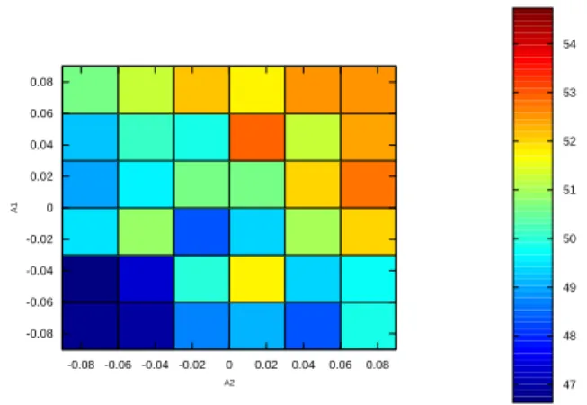
1800 times each. This is a computational cost already much bigger than in the experiment above. The un-clear results are presented in Fig. 2: the empirically best arm (0.09,0.03). 47 48 49 50 51 52 53 54 -0.08 -0.06 -0.04 -0.02 0 0.02 0.04 0.06 0.08 A2 -0.08 -0.06 -0.04 -0.02 0 0.02 0.04 0.06 0.08 A1

Figure 2: Success rate of MoGo as black against the base-line with 10s/move, as a function of the two-dimensional parameter. Here T≃ 88200 (i.e. after division by K = 49

we see that we are below the budget required for U ni f orm to work according to Eq. 7 in section 3), the sampling is nearly uniform, and the computational cost for this is al-ready around 6 times bigger than in Fig. 1 which was in the much easier case of blitz game.

We now reproduce the same experiment, but with UCB(2) (see Alg. 1) instead of uniformly sampling all the values of the parameters. ˆθ is then the arm which is most explored by UCB(2). With the same horizon, the most played arm was (0.00,0.09).

We then compared the two approaches, from the point of view ofEL(ˆθ), as shown in Table 1.

The results are significant in the sense that all al-gorithms provided an arm which significantly outper-formed the baseline (except “uniform” for which the significance is questionable), but it’s difficult to com-pare these results which are equal within 2 standard deviations and which correspond each to one run of the algorithm. We therefore switch to carefully de-signed artificial experiments.

4.4

The tuning of MoGo - extended

experiments

The purpose of this experimental section is to empir-ically support multiple claims regarding multi-armed bandit problems optimizing simple regret instead of cumulative regret.

Let us bear in mind that the goal is to get the minimal expected simple regret for a given number of pulls. (Bubeck et al., 2009) has shown that uni-formly pulling arms is asymptotically optimal in this case. Nevertheless, it has been suggested in the same paper that in practical applications, using strategies designed for cumulative regret on simple regret

prob-Algorithm Horizon Selected arm Generalization performance

Baseline 51.37 %_{± 0.3%}

UCB(2)+most played arm 88 000 (0.00,0.09) 52.65%_{± 0.3%} UCB(2)+most played arm 150 000 (0.03,0.09) 52.42%_{± 0.3%} Uniform+empirically best arm 88 000 (0.09,0.03) 52.00%_{± 0.3%}

Table 1: Comparison between the different algorithms in the non-blitz settings. In order to have more significant experiments, we will “randomize” and rerun this dataset in section 4.4.

lems often yields much better results, although those strategies are suboptimal asymptotically.

Two arm selection strategies are investigated in this section:

U ni f orm The arm selected for the nth _{arm pull is}

n%K, where K is the number of arms. Thus, all

the arms are pulled the same number of times if K is a divisor of N;

UCB(p) The nth_{arm is selected according to the}

Up-per Confidence Bound formula(Auer et al., 2002), with p being a parameter weighing the exploration term (see algorithm 1).

Algorithm 1 The UCB(p) algorithm. It plays at each round the arm with the highest upper confidence bound. Xi,sis the random reward of arm i after s pulls.

Ti(t) is the number of times i has been pulled after a

total number t of pulls. For more details see(Bubeck et al., 2009; Auer, 2003).

Algorithm UCB(p)

Input: K arms

Parameter: p accounting for the weight of explo-ration in the strategy

t=0 // current total number of arms pulled

while true do t++ for i_{∈ {1,...,K} do} if Ti(t − 1) == 0 then Bi,t= +∞ else Bi,t=µi,t−1ˆ + q _α lnt Ti(t−1) where µi,t−1=Ti(t−1)1 ∑ Ti(t−1) s=1 Xi,s end if end for

Pull any arm i_{∈ argmax}iBi,t

end while

Note that after having exhausted the allowed num-ber of pulls to choose an arm, there are various rules to decide which arm to keep (these rules are termed recommendation rules):

Empirical best arm (EBA): the arm kept is the one

with the best empirical mean;

Most played arm (MPA): the arm is the one which

has been played most;

Empirical distribution of plays (EDP): the arm is

selected by random draw among the K arms, where each arm has a probability of being chosen proportionnal to the number of times it has been played.

Here are a few remarks regarding these decision rules:

• For the Uni f orm selection strategy, MPA makes

no sense, since the first N%K arms have been played exactly once more than the remaining ones. Furthermore, EDP degenerates to randomly choosing an arm.

• For UCB-based selection strategies, or other

con-fidence bound strategies, EBA is the most aggres-sive choice, since an arm that has been played less, but that has a better average, will be pre-ferred. On the other hand, MPA will select arms in which the uncertainty on the mean is low—both are sound, however, and converge to the same re-sult for confidence-bound based selection strate-gies.

The following experiments investigate these arm selection procedures on three “almost real-world” ap-plications, designed as follows:

• We applied the Uni f orm strategy during a very

long time.

• We recorded the results.

• Then, we could simulate various strategies

“of-fline”; for each simulation, we permuted the ran-dom draws, so that there’s no systematic bias. Each problem consists in a few hundreds of arms whose rewards are bernouilli distributions with pa-rameter p close to 1/2. Experiments are performed by

confronting strategies U ni f orm, UCB(0.1), UCB(1)

and UCB(10) for each recommendation rule (EBA,

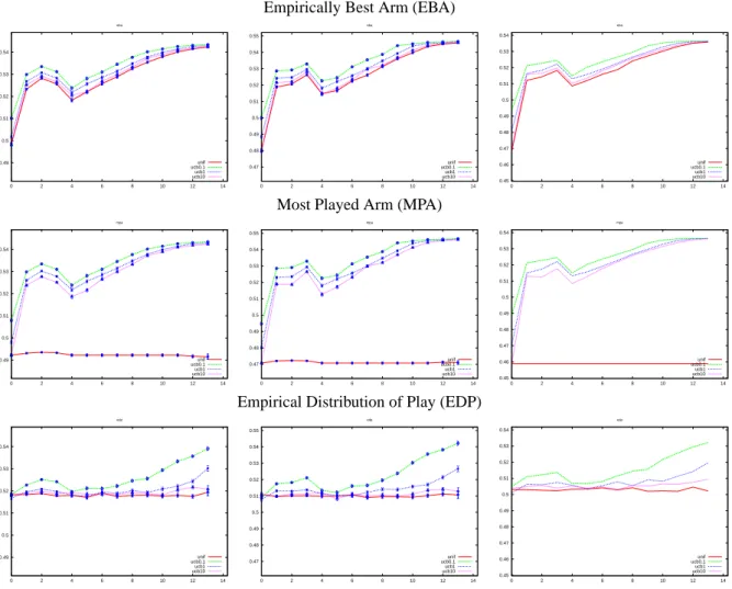
MPA and EDP). For each of the 3 experiments, each selection strategy and each decision rule, experiments were performed for various horizons (number of al-lowed pulls), going from 100 to 819200. Results are presented on Fig. 4.4 and show that (i) UCB performs

better than U ni f orm (ii) the improvement is moder-ate, in particular when the horizon exceeds the thresh-old proposed in Eq. 7. A strength of U ni f orm is that the performance is naturally evaluated on the fly for all arms; therefore both the statistical validation and the visualization are straightforward and for free.

5

DISCUSSION

We have surveyed simple regret algorithms. They are noisy optimization algorithms, and they don’t assume any structure on the domain. We compared U ni f orm (known as optimal for sufficiently large horizon, i.e. sufficiently large time budget) and UCB for automatic parameter tuning. Our results are as follows:

• MSHT (even the simple Bonferroni correction) is relevant for Automatic Parameter Tuning.

It predicts how many computational power is re-quired for U ni f orm; when the number K of tested sets of parameters depends on a discretization, MSHT can be applied for choosing the grain of the discretization. The U ni f orm approach com-bined with MSHT by Bonferroni correction might be the best approach when the computational power is large in front of K, thanks to its statis-tical guarantees, the easy visualization, the opti-mality in terms of simple regret. However, non-asymptotically, it is not optimal and the rule be-low is here for deciding the relevance of U ni f orm when K and T are known.

• Choosing between the naive solution (Uni f orm sampling) and sophisticated algorithms. The

naive U ni f orm algorithm is provably optimal for large values of the horizon. We propose the fol-lowing simple rule for choosing if it is worth using something else than the simple uniform sampling:

– Compute

s=δ√n/σ.

where

∗ δ is the amplitude of the expected change in reward;

∗ σis the expected standard deviation;

∗ n is the number of experiments you can

per-form for each arm with your computational power.

– Test if

exp_(−s2₎

s√2π ≤ 0.05/K where K is the number of arms.

– If yes, then uniform sampling is ok.

Other-wise, you can try UCB-like algorithms (but,

in that case, there’s no statistical guarantee), or Bernstein races. At first view, our choice would be Bernstein races for an implementa-tion aimed at automatically tuning and vali-dating several modifications (as in (Hoock and Teytaud, 2010)) as soon as conditions above are not met by the computational power available; if the computational power available is strong enough, U ni f orm has nice visualization prop-erties.

– What if uniform algorithms can’t do it ? If

K is not large, nothing can be much better than

uniform; at most the required horizon can be divided by K log(K). What if K is large ? UCB

is probably much better when K is large. A drawback is that it does not include any sta-tistical validation, and is not trivially paral-lel; therefore, classical algorithms derived far from the field of simple regret, like Bernstein races(Bernstein, 1924), might be more relevant. Bernstein races are close to the U ni f orm algo-rithm, except that they discard arms as early as possible (Mnih et al., 2008; Hoock and Tey-taud, 2010) by performing statistical tests on the fly. A drawback is that Bernstein races do not provide a complete picture of the search space and of the fitness landscape as U ni f orm; also, if no arm can be discarded early, the hori-zon required for statistical validation is bigger than for U ni f orm as tests are performed during the run. Yet, Bernstein races might be the most elegant tool for doing better than U ni f orm as they adapt to various frameworks(Hoock and Teytaud, 2010): when many arms can be dis-carded easily, they will save up a lot of compu-tational power.

• Results on our application to MCTS. For the

specific application, the results were significant but moderate; however, it can be pointed out that many handcrafted modifications around Monte-Carlo Tree Search provide such small improve-ments of a few percents each. Moreover, as shown in (Hoock and Teytaud, 2010), improve-ments performed automatically by bandits can be applied incrementally, leading to huge improve-ments once they are cumulated.

• Comparing recommendation techniques: most played arm is better. The empirically best arm

and the most played arm in UCB are usually the same (this is not the case for various other ban-dit algorithms), and are much better than the “em-pirical distribution of play” technique. The most played arm and the empirical distribution of play obviously do not make sense for U ni f orm. Please

Empirically Best Arm (EBA) 0.49 0.5 0.51 0.52 0.53 0.54 0 2 4 6 8 10 12 14 eba unif ucb0.1 ucb1 ucb10 0.47 0.48 0.49 0.5 0.51 0.52 0.53 0.54 0.55 0 2 4 6 8 10 12 14 eba unif ucb0.1 ucb1 ucb10 0.45 0.46 0.47 0.48 0.49 0.5 0.51 0.52 0.53 0.54 0 2 4 6 8 10 12 14 eba unif ucb0.1 ucb1 ucb10

Most Played Arm (MPA)

0.49 0.5 0.51 0.52 0.53 0.54 0 2 4 6 8 10 12 14 mpa unif ucb0.1 ucb1 ucb10 0.47 0.48 0.49 0.5 0.51 0.52 0.53 0.54 0.55 0 2 4 6 8 10 12 14 mpa unif ucb0.1 ucb1 ucb10 0.45 0.46 0.47 0.48 0.49 0.5 0.51 0.52 0.53 0.54 0 2 4 6 8 10 12 14 mpa unif ucb0.1 ucb1 ucb10

Empirical Distribution of Play (EDP)

0.49 0.5 0.51 0.52 0.53 0.54 0 2 4 6 8 10 12 14 edp unif ucb0.1 ucb1 ucb10 0.47 0.48 0.49 0.5 0.51 0.52 0.53 0.54 0.55 0 2 4 6 8 10 12 14 edp unif ucb0.1 ucb1 ucb10 0.45 0.46 0.47 0.48 0.49 0.5 0.51 0.52 0.53 0.54 0 2 4 6 8 10 12 14 edp unif ucb0.1 ucb1 ucb10

Figure 3: Simple regret strategies compared on the blitz case as black (left), blitz case as white (middle) and standard case (right) for various horizons. The Y-axis is the true mean of the arm chosen by a simple regret strategy being allowed H pulls on arms on the whole. On the X-axis lies log(H/100). Each point of each curve is the result of an average over more

than 1000 experiments; this explains the almost unoticeable 95% error bars. Consequently, even small gaps between curves are statistically significant. The order of the curves is as follows: in all cases, with≥ for ”performed better”, UCB(0.1) ≥

note that it is known in other settings (see (Wang and Gelly, 2007)) that the most played arm is bet-ter(Wang and Gelly, 2007). MPA is seemingly a reliable tool in many settings.

A next experimental step is the automatic use of the algorithm for more parameters, or e.g. by extending automatically the neural network used in the Monte-Carlo Tree Search so that it takes into account more inputs: instead of performing one big modification, apply several modifications the one after the other, and tune them sequentially so that all the modifica-tions can be visualized and checked independently. The fact that the small constant 0.1 was better in UCB

is consistant with the known fact that tuned version of UCB (with p related to the variance) provides better results; using tuned-UCB might provide further im-provements(Audibert et al., 2006).

ACKNOWLEDGEMENTS

This work has been supported by French National Re-search Agency (ANR) through COSINUS program (project EXPLO-RA No ANR-08-COSI-004), and grant No. ANR-08-COSI-007-12 (OMD project). It benefited from the help of Grid5000 for parallel ex-periments.

REFERENCES

Audibert, J.-Y., Munos, R., and Szepesvari, C. (2006). Use of variance estimation in the multi-armed bandit prob-lem. In NIPS 2006 Workshop on On-line Trading of Exploration and Exploitation.

Auer, P. (2003). Using confidence bounds for exploitation-exploration trade-offs. The Journal of Machine Learn-ing Research, 3:397–422.

Auer, P., Cesa-Bianchi, N., and Fischer, P. (2002). Finite time analysis of the multiarmed bandit problem. Ma-chine Learning, 47(2/3):235–256.

Auger, A. and Teytaud, O. (Accepted). Continuous lunches are free plus the design of optimal optimization algo-rithms. Algorithmica.

Bernstein, S. (1924). On a modification of chebyshev’s in-equality and of the error formula of laplace. Original publication: Ann. Sci. Inst. Sav. Ukraine, Sect. Math. 1, 3(1):38–49.

Bubeck, S., Munos, R., and Stoltz, G. (2009). Pure explo-ration in multi-armed bandits problems. In ALT, pages 23–37.

Chaslot, G., Hoock, J.-B., Teytaud, F., and Teytaud, O. (2009). On the huge benefit of quasi-random mu-tations for multimodal optimization with application to grid-based tuning of neurocontrollers. In ESANN, Bruges Belgium.

Chaslot, G., Saito, J.-T., Bouzy, B., Uiterwijk, J. W. H. M., and van den Herik, H. J. (2006). Monte-Carlo Strate-gies for Computer Go. In Schobbens, P.-Y., Vanhoof, W., and Schwanen, G., editors, Proceedings of the 18th BeNeLux Conference on Artificial Intelligence, Namur, Belgium, pages 83–91.

Coulom, R. (2006a). Efficient selectivity and backup oper-ators in monte-carlo tree search. In P. Ciancarini and H. J. van den Herik, editors, Proceedings of the 5th International Conference on Computers and Games, Turin, Italy.

Coulom, R. (2006b). Efficient selectivity and backup oper-ators in monte-carlo tree search. In P. Ciancarini and H. J. van den Herik, editors, Proceedings of the 5th International Conference on Computers and Games, Turin, Italy.

De Mesmay, F., Rimmel, A., Voronenko, Y., and P¨uschel, M. (2009). Bandit-Based Optimization on Graphs with Application to Library Performance Tuning. In ICML, Montr´eal Canada.

Holm, S. (1979). A simple sequentially rejective multiple test procedure. scand. j. statistic., 6:65-70.

Hoock, J.-B. and Teytaud, O. (2010). Bandit-based genetic programming. In Accepted in EuroGP 2010, LLNCS. Springer.

Hsu, J. (1996). Multiple comparisons, theory and methods, chapman & hall/crc.

Kocsis, L. and Szepesvari, C. (2006). Bandit based monte-carlo planning. In 15th European Conference on Ma-chine Learning (ECML), pages 282–293.

Lee, C.-S., Wang, M.-H., Chaslot, G., Hoock, J.-B., Rim-mel, A., Teytaud, O., Tsai, S.-R., Hsu, S.-C., and Hong, T.-P. (2009). The Computational Intelligence of MoGo Revealed in Taiwan’s Computer Go Tourna-ments. IEEE Transactions on Computational Intelli-gence and AI in games.

Mnih, V., Szepesv´ari, C., and Audibert, J.-Y. (2008). Empir-ical Bernstein stopping. In ICML ’08: Proceedings of the 25th international conference on Machine learn-ing, pages 672–679, New York, NY, USA. ACM. Nannen, V. and Eiben, A. E. (2007a). Relevance

estima-tion and value calibraestima-tion of evoluestima-tionary algorithm par ameters. In International Joint Conference on Ar-tificial Intelligence (IJCAI’07), pages 975–980. Nannen, V. and Eiben, A. E. (2007b). Variance reduction

in meta-eda. In GECCO ’07: Proceedings of the 9th annual conference on Genetic and evolutionary com-putation, pages 627–627, New York, NY, USA. ACM. Pantazis, D., Nichols, T. E., Baillet, S., and Leahy, R. (2005). A comparison of random field theory and per-mutation methods for the statistical analysis of MEG data. Neuroimage, 25:355–368.

Rolet, P., Sebag, M., and Teytaud, O. (2009). Optimal active learning through billiards and upper confidence trees in continous domains. In Proceedings of the ECML conference.

Wang, Y. and Gelly, S. (2007). Modifications of UCT and sequence-like simulations for Monte-Carlo Go. In

IEEE Symposium on Computational Intelligence and Games, Honolulu, Hawaii, pages 175–182.

Wolpert, D. and Macready, W. (1997). No Free Lunch The-orems for Optimization. IEEE Transactions on Evo-lutionary Computation, 1(1):67–82.