Constraints on the richness–mass relation and the
optical-SZE positional offset distribution for optical-SZE-selected clusters
The MIT Faculty has made this article openly available.
Please share
how this access benefits you. Your story matters.
Citation
Saro, A. et al. “Constraints on the Richness–mass Relation and
the Optical-SZE Positional Offset Distribution for SZE-Selected
Clusters.” Monthly Notices of the Royal Astronomical Society 454.3
(2015): 2305–2319.
As Published
http://dx.doi.org/10.1093/mnras/stv2141
Publisher
Oxford University Press
Version
Original manuscript
Citable link
http://hdl.handle.net/1721.1/108814
Terms of Use
Creative Commons Attribution-Noncommercial-Share Alike
Constraints on the Richness-Mass Relation and the Optical-SZE
Positional O
ffset Distribution for SZE-Selected Clusters
A. Saro
1,2, S. Bocquet
1,2, E. Rozo
3, B. A. Benson
4,5,6, J. Mohr
1,2,7, E. S. Ryko
ff
8,9,
M. Soares-Santos
4, L. Bleem
5,10, S. Dodelson
4,5,6, P. Melchior
11,12, F. Sobreira
4,13,
V. Upadhyay
14, J. Weller
2,7,15, T. Abbott
16, F. B. Abdalla
17, S. Allam
4, R. Armstrong
18,
M. Banerji
19, A.H. Bauer
20, M. Bayliss
21,22, A. Benoit-L´evy
17, G. M. Bernstein
18,
E. Bertin
23, M. Brodwin
24, D. Brooks
17, E. Buckley-Geer
4, D. L. Burke
8,9,
J. E. Carlstrom
5,6,25, R. Capasso
1,2, D. Capozzi
26, A. Carnero Rosell
13,27,
M. Carrasco Kind
28,29, I. Chiu
1,2, R. Covarrubias
29, T. M. Crawford
5,6, M. Crocce
20,
C. B. D’Andrea
26, L. N. da Costa
13,27, D. L. DePoy
30, S. Desai
1, T. de Haan
31,32,
H. T. Diehl
4, J. P. Dietrich
1,2, P. Doel
17, C. E Cunha
8, T. F. Eifler
18,33,
A. E. Evrard
34,35, A. Fausti Neto
13, E. Fernandez
36, B. Flaugher
4, P. Fosalba
20,
J. Frieman
4,5, C. Gangkofner
1,2, E. Gaztanaga
20, D. Gerdes
35, D. Gruen
7,15,
R. A. Gruendl
28,29, N. Gupta
1,2, C. Hennig
1,2, W. L. Holzapfel
32, K. Honscheid
11,12,
B. Jain
18, D. James
16, K. Kuehn
37, N. Kuropatkin
4, O. Lahav
17, T. S. Li
30, H. Lin
4,
M. A. G. Maia
13,27, M. March
18, J. L. Marshall
30, Paul Martini
11,38, M. McDonald
39,
C.J. Miller
34,35, R. Miquel
36, B. Nord
4, R. Ogando
13,27, A. A. Plazas
33,40,
C. L. Reichardt
32,41, A. K. Romer
42, A. Roodman
8,9, M. Sako
18, E. Sanchez
43,
M. Schubnell
35, I. Sevilla
28,43, R. C. Smith
16, B. Stalder
22,44, A. A. Stark
22,
V. Strazzullo
1,2, E. Suchyta
11,12, M. E. C. Swanson
29, G. Tarle
35, J. Thaler
45,
D. Thomas
26, D. Tucker
4, V. Vikram
10, A. von der Linden
46, A. R. Walker
16,
R. H. Wechsler
8,9,46, W. Wester
4, A. Zenteno
47, K. E. Ziegler
5Affiliations are listed at the end of the paper
Accepted ???. Received ???; in original form ???
ABSTRACT
We cross-match galaxy cluster candidates selected via their Sunyaev-Zel’dovich effect (SZE) signatures in 129.1 deg2of the South Pole Telescope 2500d SPT-SZ survey with optically identified clusters selected from the Dark Energy Survey (DES) science verification data. We identify 25 clusters between 0.1. z . 0.8 in the union of the SPT-SZ and redMaPPer (RM) samples. RM is an optical cluster finding algorithm that also returns a richness estimate for each cluster. We model the richness λ-mass relation with the following function hln λ|M500i ∝
Bλln M500+ Cλln E(z) and use SPT-SZ cluster masses and RM richnesses λ to constrain the
parameters. We find Bλ = 1.14+0.21−0.18 and Cλ = 0.73+0.77−0.75. The associated scatter in mass at fixed richness is σln M|λ = 0.18+0.08−0.05at a characteristic richness λ= 70. We demonstrate that
our model provides an adequate description of the matched sample, showing that the fraction of SPT-SZ selected clusters with RM counterparts is consistent with expectations and that the fraction of RM selected clusters with SPT-SZ counterparts is in mild tension with expectation. We model the optical-SZE cluster positional offset distribution with the sum of two Gaussians, showing that it is consistent with a dominant, centrally peaked population and a sub-dominant population characterized by larger offsets. We also cross-match the RM catalog with SPT-SZ candidates below the official catalog threshold significance ξ = 4.5, using the RM catalog to provide optical confirmation and redshifts for additional low-ξ SPT-SZ candidates. In this way, we identify 15 additional clusters with ξ ∈ [4, 4.5] over the redshift regime explored by
c
0000 RAS
1 INTRODUCTION
Clusters of galaxies were first identified as over-dense regions in the projected number counts of galaxies (e.g., Abell 1958; Zwicky et al. 1968). Nowadays, clusters are also regularly identified through their X-ray emission (e.g., Gioia et al. 1990; Vikhlinin et al. 1998; B¨ohringer et al. 2000; Pacaud et al. 2007; ˇSuhada et al. 2012) and at millimeter wavelengths through their Sunyaev-Zel’dovich effect (SZE) signatures (Sunyaev & Zel’dovich 1972). Large, homoge-neously selected samples of clusters are useful for both cosmologi-cal and astrophysicosmologi-cal studies, and such samples have recently begun to be produced using SZE selection (Staniszewski et al. 2009; Has-selfield et al. 2013; Planck Collaboration et al. 2015; Bleem et al. 2015b). There is a longer history of large cluster samples selected from optical and near infrared photometric surveys (e.g., Gladders & Yee 2000; Koester et al. 2007; Eisenhardt et al. 2008; Menanteau et al. 2010; Hao et al. 2010; Wen et al. 2012; Rykoff et al. 2014; Bleem et al. 2015a; Ascaso et al. 2014, and references therein), and even larger samples will soon be available from ongoing and fu-ture surveys like the Dark Energy Survey (DES, The Dark Energy Survey Collaboration 2005)1, KiDS (de Jong et al. 2013), Euclid
(Laureijs et al. 2011) and LSST (LSST Dark Energy Science Col-laboration 2012).
Reliable estimates of galaxy cluster masses play a key role in both cosmological and astrophysical cluster studies. First, the abundance of galaxy clusters as a function of mass is a well-known cosmological probe (White et al. 1993; Bartlett & Silk 1994; Eke et al. 1998; Viana & Liddle 1999; Borgani et al. 2001; Vikhlinin et al. 2009; Rozo et al. 2010; Mantz et al. 2010; Allen et al. 2011; Benson et al. 2013; Bocquet et al. 2015, and many others). Second, accurate estimates of cluster masses are crucial in disentangling environmental effects from the secular evolution processes shaping galaxy formation (Mei et al. 2009; Zenteno et al. 2011; Muzzin et al. 2012).
In this paper, we calibrate the richness-mass relation for SZE-selected galaxy clusters detected in the DES science verification data (SVA1) using the redMaPPer (Rykoff et al. 2014) cluster-finding algorithm. Specifically, we study the clusters detected via their SZE signatures in the South Pole Telescope SPT-SZ cluster survey (Bleem et al. 2015b, hereafter B15) that are also present in the redMaPPer catalog. We also study the distribution of offsets between the SZE derived centres and the associated optical cen-tres, properly including the SZE positional uncertainties. Finally, we demonstrate our ability to push to even lower candidate signifi-cance within the SPT-SZ candidate catalog by taking advantage of the contiguous, deep, multiband imaging available through DES. In this respect, our study points towards the combined use of DES and SPT datasets to provide highly reliable extended SZE-selected clus-ter samples. We note that historically the optical follow-up of SPT selected clusters was the original motivation for proposing DES.
The plan of the paper is as follows. In Section 2 we describe the galaxy cluster catalogs and the matching metric we use in this work. Section 3 describes the method we adopt to calibrate the SZE-mass and richness-mass relations. Our results are presented in Section 4. Section 5 contains a discussion of our findings and our conclusions. In the Appendix, we provide a preliminary analy-sis of a cluster sample created using an independent cluster finding algorithm — the Voronoi Tessellation (VT) cluster finder — which helps to highlight areas where the VT algorithm can be improved. Throughout this work, we adoptΩM = 0.3, ΩΛ = 0.7, H0 = 70
1 http://www.darkenergysurvey.org
km s−1 Mpc−1, and σ
8 = 0.8. Cluster masses are defined within
R500, the radius within which the density is 500 times the
criti-cal density of the Universe. Future analyses will include the de-pendence of the derived scaling relation parameters on the adopted cosmology by simultaneously fitting for cosmological and scaling-relation parameters (e.g. Mantz et al. 2010; Rozo et al. 2010; Boc-quet et al. 2015).
2 CLUSTER SAMPLE 2.1 SPT-SZ Cluster Catalog
The SPT-SZ galaxy cluster sample used in this analysis has been selected via the cluster thermal SZE signatures in a point-source masked-region of 2365 deg2of the 2540 deg2(2500d) SPT-SZ sur-vey using 95 GHz and 150 GHz data. Typical instrumental noise is approximately 40 (18) µKCMB-arcmin and the beam FWHM is
1.6 (1.2) arcmin for the 95 (150) GHz maps. A multi-frequency matched filter is used to extract the cluster SZE signal in a manner designed to optimally measure the cluster signal given knowledge of the cluster profile, the SZE spectrum and the noise in the maps (Haehnelt & Tegmark 1996; Melin et al. 2006). The cluster gas profiles are assumed to be described by a projected isothermal β model (Cavaliere & Fusco-Femiano 1976) with β= 1. Note that, as discussed in Vanderlinde et al. (2010), the resulting SPT-SZ can-didate catalogs are not sensitive to this assumption. The adopted model provides a SZE temperature decrement that is maximum at the cluster centre and weakens with separation θ from the cluster centre as:
∆T(θ) = ∆T0[1+ (θ/θc)2]−1, (1)
where∆T0is the central value and θcis the core radius. We adopt
12 different cluster profiles linearly spaced from θc = 0.25 to 3
arcmin (Vanderlinde et al. 2010; Reichardt et al. 2013, B15). For each cluster, the maximum signal-to-noise across the 12 filtered maps is denoted as ξ. The SPT-SZ cluster candidates with ξ > 4.5 have been previously published in B15.
2.2 DES Optical Cluster Catalogs
The DES Science Verification Data (DES-SVA1) that overlap SPT have been used to produce optically selected catalogs of clusters. In Section 2.2.1 we describe the acquisition and preparation of the DES-SVA1 data, and in Section 2.2.2 we describe the production of the redMaPPer cluster catalog used in the primary analysis. We remind the reader that in Appendix A we present results of a pre-liminary analysis of the VT cluster catalog.
2.2.1 DES-SVA1 Data
The DES-SVA1 data include imaging of ∼ 300 deg2over multi-ple disconnected fields (Melchior et al. 2015; S´anchez et al. 2014; Banerji et al. 2015), most of which overlap with the SPT-SZ survey. The DES-SVA1 data were acquired with the Dark Energy Camera (Diehl T. et al. 2012; Flaugher et al. 2012, 2015) over 78 nights, starting in Fall 2012 and ending early in 2013 with depth compa-rable to the nominal depth of the full DES survey (Rykoff et al., in preparation).
Data have been processed through the DES Data Manage-ment (DESDM, Desai et al. 2012) pipeline that is an advanced version of development versions described in several publications
(Ngeow et al. 2006; Mohr et al. 2008, 2012). The data were cal-ibrated in several stages leading to a Gold catalog of DES-SVA1 galaxies (Rykoff et al., in preparation). The Gold catalog covers ∼ 250 deg2and is optimized for extragalactic science. In particular it masks regions south of declination δ= −61◦, avoiding the Large
Magellanic Cloud and its high stellar densities. Furthermore, the footprint is restricted to the regions where we have coverage in all four bands.
2.2.2 redMaPPer Cluster Catalog
The red-sequence Matched-Filter Probabilistic Percolation (redMaPPer, hereafter RM) algorithm is a cluster-finding algo-rithm based on the richness estimator of Rykoff et al. (2012). RM has been applied to photometric data from the Eighth Data Release (DR8) of the Sloan Digital Sky Survey (Aihara et al. 2011, SDSS,) and to the SDSS Stripe 82 coadd data (Annis et al. 2014), and has been shown to provide excellent photometric redshifts, richness estimates that tightly correlate with external mass proxies, and very good completeness and purity (Rozo & Rykoff 2014; Rozo et al. 2014b,c). We refer the reader to the paper by Rykoff et al. (2014) for a detailed description of the algorithm. Here, we briefly summarize the most salient features.
We employ an updated version of the algorithm (v6.3.3), with improvements summarized in Rozo & Rykoff (2014), Rozo et al. (2015, in preparation), and Rykoff et al. (2015, in preparation). RM calibrates the colour of red-sequence galaxies using galaxy clus-ters with spectroscopic redshifts. RM uses this information to esti-mate the membership probability of every galaxy in the vicinity of a galaxy cluster. The richness λ is thus defined as the sum of the membership probabilities (pRM) over all galaxies:
λ =X
pRM. (2)
In addition to the estimate of membership probabilities, the RM centering algorithm is also probabilistic. The centering probabil-ity Pcen is a likelihood-based estimate of the probability that the
galaxy under consideration is a central galaxy. The centering like-lihood includes the fact that the photometric redshift of the central galaxy must be consistent with the cluster redshift, that the central galaxy luminosity must be consistent with the expected luminos-ity of the central galaxy of a cluster of the observed richness, and that that the galaxy density on a 300 kpc scale consistent with the galaxy density of central galaxies. The centering probability fur-ther accounts for the fact that every cluster has one and only one central galaxy, properly accounting for the relevant combinatoric factors. These probabilities have been tested on SDSS DR8 data using X-ray selected galaxy clusters, and have been shown to pro-duce cluster centres that are consistent with the X-ray centres (Rozo & Rykoff 2014).
The DES-SVA1 RM catalog was produced by running on a smaller footprint than that for the full SVA1 Gold sample. In par-ticular, we restrict the catalog to the regions where the z-band 10σ galaxy limiting magnitude is z > 22. In total, we use 148 deg2 of
DES-SVA1 imaging, with 129.1 deg2overlapping the SPT-SZ foot-print. In this area, the largest fraction (124.6 deg2) is included in
the so called DES-SVA1 SPT-E field. The final catalog used in this work consists of 9281 clusters with λ > 5 and redshifts in the range 0.1 < z < 0.9. Due to the varying depth of the DES-SVA1 cata-log, RM produces a mask that determines the maximum redshift of the cluster search at any given location in the survey. As an ex-ample, the effective area in the SPT-E region at the highest redshift (z > 0.85) is only ∼ 30 deg2. In addition to the cluster catalog, the
RM algorithm also uses the survey mask to produce a set of random points with the same richness and redshift distribution as the clus-ters in the catalog. The random points take into account the survey geometry and the physical extent of the clusters, and as with the clusters, only includes points that have < 20% of the local region masked (see Rykoff et al. 2014).
2.3 Catalog Matching
We cross-match the SPT-SZ catalog with the RM optical cluster catalog following the method of Rozo et al. (2014c). First, we sort the SPT-SZ clusters to produce a list with decreasing SZE observ-able ξ, and we sort the RM catalog to produce a list with decreasing richness. Second, we go down the SPT-SZ sorted list, associating each SPT cluster candidate with the richest RM cluster candidate whose centre lies within 1.5 R500 of the SZE centre. Third, we
re-move the associated RM cluster from the list of possible counter-parts when matching the remaining SPT-selected clusters.
R500 is first computed assuming the redshift of the optical
counterpart and using the SZE-mass scaling relation parameters adopted in B15. We subsequently check that our sample does not change when adopting our best fitting scaling relation parameters (see Section 3.1).
To test the robustness of our matching algorithm against chance associations, we first perform the above described proce-dure on a sample of randomly generated RM clusters as described in the previous Section. Positions of clusters in this randomly gen-erated sample do not correlate with the positions of the SPT-SZ clusters. Using an ensemble of 104 random catalogs we measure
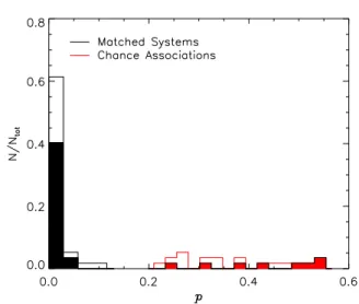
the distribution of richness in chance associations for each SPT-SZ candidate. We then apply the algorithm to match the real RM clus-ter catalog with the SPT-SZ candidate list where ξ > 4.5. The distri-bution of probabilities p of chance associations estimated for each cluster candidate using the randomly generated samples is shown in Figure 1 (filled histogram).
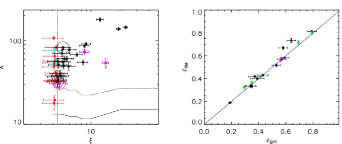
In Figure 2 (left panel) we show the resulting 84% and 95% confidence limits (solid and dotted lines, respectively) in the rich-ness distribution of the chance associations as a function of the SPT-SZ observable ξ. This test allows us to estimate the proba-bility of chance superposition for each SPT-SZ cluster candidate. As detailed below, we use this information to determine whether or not to include particular matches for further analysis. As Fig-ure 2 shows, this filtering of the matched sample then ensFig-ures that chance superpositions are playing no more than a minor role even at 4 < ξ < 4.5.
Within the DES-SVA1 region explored by RM there are 36 such SPT-SZ cluster candidates. Using information on the contam-ination fraction at ξ > 4.5 of the SPT-SZ candidate list and on the redshift distribution of the confirmed cluster candidates (Song et al. 2012, B15), we expect ∼ 9 of these candidates to be noise fluctu-ations and ∼ 80% of the real clusters to lie at z < 0.8. Therefore, assuming the optical catalog is complete, the expected number of real cluster matches is ∼ 22. Similarly, one can estimate an ex-pected number of real cluster matches (23.6) by scaling the total number of confirmed clusters in B15 below z = 0.8 (433) in the 2365 deg2of the SPT-SZ survey by the DES-SVA1 area overlap-ping SPT-SZ that has been processed with the RM cluster finder (129.1 deg2).
The actual number of matches to the SPT-SZ candidates is 33. Eight systems are foreground, low-richness RM clusters that have been erroneously associated with SPT-SZ candidates with either previously measured redshifts (four systems) or lower limits
esti-Figure 1. Distribution of probability p of chance associations for the ξ > 4.5 (filled) and ξ > 4 (empty) samples. Black lines show the sample used in this work, red lines show the sample rejected (Section 2.3).
mated in B15 (the remaining four candidates) that are at z& 0.8; these systems are either noise fluctuations or real clusters that are at redshifts too high for them to be detected by RM. In fact, all of these systems have a probability p of chance associations estimated from the randomly generated sample that is p > 16%. Therefore, we remove these matches from the sample. This leaves 25 SPT-SZ candidates at ξ > 4.5 that have RM counterparts. We expect less than one false associations within this sample of 25 candidates. The associated optical richness as a function of the SPT-SZ sig-nificance is shown in the left panel of Figure 2. This number is somewhat larger but statistically consistent with the expected num-ber of matches presented above. All 22 of the SPT-SZ confirmed clusters presented in B15 that lie at redshifts where they could be detected by RM are in this matched sample. According to our matching metric (which differs from the approach in B15), there are also three unconfirmed SPT-SZ candidates (i.e., candidates without identified optical counterparts in the B15 analysis) that have RM counterparts: CL J0502-6048, CL J0437-5307 and SPT-CL J0500-4551. The newly confirmed clusters are highlighted with large circles in Figure 2.
Of the 25 SPT-SZ candidates with robust RM counterparts, we use 19 of them to calibrate the RM richness-mass relation. Six clusters are excluded from the analysis for the following rea-sons. Clusters with estimated redshift z < 0.25 in the SPT-SZ catalog from B15 are highlighted in cyan in the left panel of Fig-ure 2. Because the ξ-mass relation is robust only above this redshift (Vanderlinde et al. 2010), these systems are not used in the fol-lowing analysis. Two systems (SPT-CL J0440-4744 and SPT-CL J0441-4502) are excluded from this analysis as they are detected in SPT-SZ regions that have been masked due to their proximity to point sources, which can compromise the SZE signal-to-noise mea-surement. In addition, we exclude the three clusters highlighted in magenta: SPT-CL J0417-4748, SPT-CL J0456-5116 and SPT-CL J0502-6048. These systems are strongly masked in the DES-SVA1 data; based on the SZE position, the masks cover 40% of the to-tal cluster region. As a result, the associated optical counterparts are highly mis-centered, and the corresponding richness is severely biased. We note that the average centering failure rate caused by the detection mask is 12% (3 clusters out of 25), in comparison to
the corresponding rate in the SDSS RM catalog, which is ≈1% -2%. The difference reflects the fact that SDSS has a much larger contiguous area, while SVA1 has a more aggressive star mask. We expect this failure rate will decrease as the DES coverage increases, and object masking improves. Furthermore, improvements will be made to the RM algorithm to estimate the masked area not only at the putative centre of the cluster, but at all possible centres. In this way, clusters at high risk of mask-induced mis-centering will be properly removed from the sample.
The B15 catalog contains only SPT-SZ candidates with ξ > 4.5. In this work we also apply the matching algorithm to SPT-SZ candidates at 4 < ξ < 4.5. We identify 26 matches in this signal to noise range. The resulting probabilities of chance associations of the ξ > 4 sample are shown as empty histograms in Figure 1. Sim-ilarly to the ξ > 4.5 case, we exclude 11 of these systems, which have estimated probabilities p of chance associations p > 16%. For the 15 matched systems, the expected number of false associ-ations is also smaller than one. The remaining cleaned sample is shown as red points on the left panel of Figure 2. The resulting to-tal number of SPT-SZ and RM associations at ξ > 4 is 40. This number is in good agreement with the expectation (∼ 36) obtained using the number of SPT-candidates above ξ > 4 in the DES-SVA1 region explored by RM (88) and correcting it by the expected num-ber of noise fluctuations (∼ 45) and the numnum-ber of clusters above z> 0.8 (∼7). We find that two ξ < 4.5 SPT-SZ candidates, SPT-CL J0501-4717 and SPT-CL J0439-5611, have probabilities of random associations larger than 5%, and therefore it is not clear whether these low richness associations are correct (see Figure 2).
The right panel of Figure 2 contains a comparison of the redshifts from the RM catalogs with the redshifts published in B15 (zSPT) for the same clusters (obtained through dedicated
op-tical/NIR followup by the SPT team or taken from the literature). Clusters with spectroscopic redshifts are highlighted in green. We note that the redshift estimates are not biased for the clusters af-fected by masking (magenta points). For SPT-SZ candidates with 4 < ξ < 4.5 the SPT collaboration did not complete followup opti-cal imaging, and therefore we adopt the redshifts of the RM optiopti-cal cluster counterpart.
Table 1 contains all SPT candidates with RM counterparts used in this work. For newly confirmed SPT-SZ clusters , the as-sociated zSPTredshift is not given. We caution that the masses for
low-redshift clusters (z < 0.25) may be underestimated due to fil-tering that is done to remove the noise component associated with the primary CMB.
3 MASS CALIBRATION METHOD
We apply the method described in Bocquet et al. (2015) to char-acterize the λ-mass relation of SPT-selected clusters. We refer the reader to the original paper for a detailed description of the method. A similar approach has been adopted by Liu et al. (2015) for study-ing the SZE properties of an X-ray selected cluster sample from the XMM-BCS survey ( ˇSuhada et al. 2012; Desai et al. 2012). In this analysis, we consider the RM richness as a follow-up observ-able to the SZE-selected cluster sample. This choice is adequate as
2 SPT-CL J0423-5506 was previously identified in Song et al. (2012) and
Reichardt et al. (2012) at a redshift z= 0.21±0.04 with a signal-to-noise ξ = 4.51. The associated redshift estimated with the same analysis presented in B15 is z= 0.25 ± 0.036.
Figure 2. Left panel: Richness as a function of the SZE significance ξ for the matched cluster sample. SPT-SZ candidates with ξ < 4.5 (vertical line) are shown in red. Clusters at z < 0.25 (cyan) and clusters with miscentering due to a high masked fraction (magenta) are not used in the richness analysis. Large circles indicate the newly confirmed SPT-SZ candidates with ξ > 4.5. Solid and dashed lines represent the upper 84 and 95 percentiles in richness of chance associations of SPT-SZ candidates and clusters from the randomly generated RM catalog. Right panel: The estimated redshift for the RM sample as a function of SPT redshifts as presented in B15 from independent optical follow-up data. SPT-SZ candidates with spectroscopic redshift are shown in green. Magenta symbols are the same as in the left panel.
there are no SPT-SZ candidates with ξ > 4.5 missing RM counter-parts in the redshift and spatial regime explored by the RM catalog, so that the cross-sample can indeed be thought of as solely SPT-selected. We note that this is not the case for SPT-SZ candidates with 4 < ξ 6 4.5 that do not have RM counterparts. However, the adopted method is also accurate under the assumption that cross-matching the SPT-SZ candidate list with the RM cluster catalog cleansthe SPT-SZ candidate list, removing the expected noise fluc-tuations. Within this context the resulting cluster sample is there-fore drawn from the halo mass function through the SPT-SZ selec-tion in the redshift range explored by the RM catalog.
In the following subsections we describe the model we use to simultaneously constrain the SZE-mass relation (Section 3.1) and the richness-mass relation (Section 3.2).
3.1 The SZE-mass Relation
Following previous SPT papers (Vanderlinde et al. 2010; Benson et al. 2013; Reichardt et al. 2013; Bocquet et al. 2015, B15), we de-fine the unbiased SZE significance ζ as the average signal-to-noise a cluster would produce over many realizations of SPT data, if the cluster position and core radius were perfectly known. This quan-tity is related to the expectation value of ξ over many realizations of the SPT data by:
ζ = p
hξi2− 3, (3)
where the bias in hξi is due to maximizing the signal-to-noise over three variables (cluster right ascension, declination, and core ra-dius). The scatter of the actual observable ξ with respect to hξi is characterized by a Gaussian of unit width. The SPT observable-mass relation P(ζ|M500, z) is modeled as a log-normal distribution
of mean
hlnζ|M500, zi = lnASZE+ BSZEln
M500 3 × 10¹⁴h−1M ! +CSZEln E(z) E(z= 0.6) ! (4)
and scatter DSZE, and where E(z) ≡ H(z)/H0. At low significance
ζ . 2, there is a non-negligible chance of multiple low-mass clus-ters overlapping within the same resolution element of the SPT beam. We account for this by only considering the brightest of these objects per approximate resolution element and we compute P(ζmax|ζ) following Crawford et al. (2010). The SPT
observable-mass relation is therefore expanded to P(ζmax|ζ)P(ζ|M500, z) and
ζmaxis then converted to the observable ξ as in Eq.3.
To calibrate the ζ–M relation we use the subsample of clusters with ξ > 5 and z > 0.25 from the 2500d SPT-SZ catalog (B15). We determine the parameter values by abundance-matching the cata-log against our fixed reference cosmocata-logy. We predict the expected number of clusters as a function of mass and redshift using the halo mass function (Tinker et al. 2008). We convolve this mass function with the observable-mass relation accounting for its associated un-certainties, and compare the prediction with the data. Our approach here is effectively the opposite of the typical analysis, where cos-mological parameters are deduced from the cluster sample using both priors and calibrating information to constrain the scaling re-lation parameters (e.g. Benson et al. 2013; Bocquet et al. 2015); here, we assume perfect knowledge of cosmology to calibrate the scaling relation. Note that this method does not depend on any as-sumptions about hydrostatic equilibrium.
We assume flat priors on ASZE, BSZE, CSZEand a Gaussian prior
on DSZE= 0.18 ± 0.07; the latter corresponds to the posterior
dis-tribution derived from the cosmological analysis of the full SPT sample (de Haan et al., in preparation). We obtain the following parameters for the ζ-mass relation by maximizing the likelihood of obtaining the observed sample in ξ and redshift under the model
Table 1. SPT-SZ cluster candidates with RM counterpart. We report the SPT-ID (1), right ascension (2) and declination (3), SPT peak detection significance ξ (4), corresponding core radius (5), richness λ (6), associated redshift from the RM catalog (7) and SPT catalog (8), and SPT derived masses (9). Coordinates are J2000.
SPT ID R.A. DEC ξ θc[arcmin] λ zRM zSPT M500[1014h−170M ]
SPT-CL J0438-5419 69.574 −54.319 22.88 0.50 144.76 ± 5.52 0.42 ± 0.01 0.42 10.19 ± 1.33 SPT-CL J0040-4407 10.199 −44.133 19.34 0.50 137.45 ± 7.03 0.37 ± 0.01 0.35 9.71 ± 1.28 SPT-CL J0417-4748 64.344 −47.812 14.24 0.25 54.22 ± 6.75 0.58 ± 0.01 0.58 7.41 ± 1.00 SPT-CL J0516-5430 79.149 −54.510 12.41 1.50 178.93 ± 8.71 0.33 ± 0.02 0.29 7.05 ± 0.97 SPT-CL J0449-4901 72.273 −49.023 8.91 0.50 91.37 ± 4.75 0.80 ± 0.01 0.79 5.24 ± 0.78 SPT-CL J0456-5116 74.115 −51.275 8.58 1.00 73.08 ± 5.39 0.56 ± 0.01 0.56 5.39 ± 0.81 SPT-CL J0441-4855 70.450 −48.917 8.56 0.50 86.96 ± 4.55 0.81 ± 0.01 0.79 ± 0.04 5.10 ± 0.77 SPT-CL J0439-4600 69.807 −46.012 8.28 0.25 55.18 ± 3.52 0.34 ± 0.02 0.34 ± 0.04 5.52 ± 0.84 SPT-CL J0440-4657 70.229 −46.964 7.13 1.25 67.95 ± 3.62 0.33 ± 0.02 0.35 ± 0.04 4.95 ± 0.81 SPT-CL J0447-5055 71.843 −50.921 5.97 0.25 77.84 ± 5.26 0.40 ± 0.01 0.39 ± 0.05 4.24 ± 0.81 SPT-CL J0422-5140 65.591 −51.674 5.86 1.00 49.28 ± 5.32 0.58 ± 0.01 0.59 ± 0.03 3.98 ± 0.78 SPT-CL J0439-5330 69.928 −53.502 5.61 0.75 60.77 ± 3.81 0.43 ± 0.01 0.43 ± 0.04 3.97 ± 0.81 SPT-CL J0433-5630 68.249 −56.502 5.32 1.75 60.75 ± 4.82 0.71 ± 0.02 0.69 3.56 ± 0.78 SPT-CL J0535-5956 83.791 −59.939 5.20 0.25 50.25 ± 4.09 0.67 ± 0.02 0.58 ± 0.03 3.46 ± 0.77 SPT-CL J0440-4744 70.242 −47.736 5.12 1.25 82.55 ± 3.80 0.30 ± 0.02 − 3.75 ± 0.83 SPT-CL J0428-6049 67.026 −60.828 5.11 1.25 55.91 ± 5.95 0.73 ± 0.02 0.64 ± 0.03 3.46 ± 0.79 SPT-CL J0444-4352 71.162 −43.872 5.01 1.50 70.53 ± 5.91 0.57 ± 0.01 0.57 ± 0.03 3.53 ± 0.82 SPT-CL J0458-5741 74.598 −57.695 4.87 2.50 37.90 ± 2.68 0.19 ± 0.01 0.19 ± 0.02 3.69 ± 0.85 SPT-CL J0534-5937 83.606 −59.625 4.74 0.25 40.43 ± 3.42 0.58 ± 0.01 0.58 3.15 ± 0.76 SPT-CL J0502-6048 75.724 −60.810 4.69 0.25 30.73 ± 4.32 0.79 ± 0.02 − 3.03 ± 0.76 SPT-CL J0441-4502 70.345 −45.040 4.62 2.50 51.22 ± 4.11 0.15 ± 0.01 − 3.49 ± 0.85 SPT-CL J0429-5233 67.430 −52.559 4.56 0.75 33.84 ± 3.97 0.52 ± 0.01 0.53 ± 0.03 3.15 ± 0.79 SPT-CL J0452-4806 73.002 −48.108 4.52 0.50 56.54 ± 4.89 0.42 ± 0.01 0.37 ± 0.04 3.26 ± 0.81 SPT-CL J0437-5307 69.259 −53.119 4.51 0.25 36.89 ± 3.56 0.29 ± 0.02 − 3.20 ± 0.80 SPT-CL J0500-4551 75.209 −45.856 4.51 0.75 32.68 ± 4.82 0.26 ± 0.01 − 3.66 ± 0.91 SPT-CL J0453-5027 73.307 −50.451 4.47 0.25 31.99 ± 3.44 0.77 ± 0.02 − 2.89 ± 0.74 SPT-CL J0449-4440 72.473 −44.672 4.37 0.75 54.50 ± 5.43 0.15 ± 0.00 − 3.42 ± 0.86 SPT-CL J0423-55062 65.809 −55.104 4.36 1.25 38.65 ± 3.44 0.27 ± 0.02 − 3.26 ± 0.83 SPT-CL J0451-5057 72.937 −50.965 4.34 0.50 83.11 ± 4.62 0.76 ± 0.01 − 2.81 ± 0.74 SPT-CL J0438-4629 69.564 −46.488 4.31 0.50 41.01 ± 3.37 0.43 ± 0.01 − 3.07 ± 0.79 SPT-CL J0456-4531 74.099 −45.523 4.30 0.25 32.45 ± 3.18 0.29 ± 0.02 − 3.17 ± 0.81 SPT-CL J0431-5353 67.970 −53.896 4.22 0.50 57.23 ± 4.76 0.75 ± 0.02 − 2.74 ± 0.73 SPT-CL J0501-4717 75.274 −47.294 4.20 3.00 19.47 ± 2.50 0.35 ± 0.02 − 3.34 ± 0.88 SPT-CL J0518-5740 79.507 −57.670 4.19 0.25 65.22 ± 4.82 0.82 ± 0.01 − 2.60 ± 0.70 SPT-CL J0438-4907 69.655 −49.117 4.19 1.75 76.20 ± 4.16 0.24 ± 0.01 − 3.13 ± 0.81 SPT-CL J0513-5901 78.273 −59.029 4.17 0.25 33.29 ± 3.58 0.61 ± 0.01 − 2.75 ± 0.73 SPT-CL J0451-4910 72.888 −49.178 4.14 0.25 54.10 ± 4.10 0.73 ± 0.02 − 2.71 ± 0.73 SPT-CL J0439-5611 69.978 −56.192 4.14 0.50 17.82 ± 2.93 0.28 ± 0.02 − 3.10 ± 0.81 SPT-CL J0532-5752 83.237 −57.877 4.11 0.50 48.49 ± 3.81 0.77 ± 0.02 − 2.59 ± 0.71 SPT-CL J0449-5908 72.472 −59.142 4.11 1.25 107.14 ± 5.29 0.77 ± 0.01 − 2.68 ± 0.73
derived from Eq. 3 and Eq. 4. The results are ASZE= 4.02 ± 0.16, BSZE= 1.71 ± 0.09,
CSZE= 0.49 ± 0.16, DSZE= 0.20 ± 0.07. (5)
For every cluster in the sample we also calculate the associated mass distribution, accounting for selection effects:
P(M500|ξ, z, ~p) ∝ P(ξ|M500, z, ~p) P(M500|z, ~p), (6)
where the vector ~pencapsulates cosmological and scaling relation parameters and P(ξ|M500, z, ~p) is obtained from the ξ-mass
scal-ing relation as described by Eq. 3 and 4. The halo mass function P(M500|z, ~p) is the prior on the mass distribution at redshift z.
Masses derived for the matched cluster sample are shown in Table 1. We note that both these masses and the SZE scaling rela-tion parameters quoted here are different from the ones reported in B15. We adopt the same fixed cosmology as in B15, but in this anal-ysis we consider data from the full SPT-SZ cluster-survey as op-posed to just the sample from the initial 720 deg2(Reichardt et al. 2013).
3.2 Richness-mass Relation
As for the SZE-mass relation (Eq. 4), we assume a power law form for the λ-mass relation:
hlnλ|M500, zi = lnAλ+ Bλln M500 3 × 10¹⁴h−1M ! +Cλln E(z) E(z= 0.6) ! (7) where Aλis the normalization, Bλ characterizes the mass depen-dence, and Cλ characterizes the redshift evolution. An additional
parameter Dλdescribes the intrinsic scatter in λ, which is assumed to be log-normal and uncorrelated with the SZE scatter, with vari-ance given by:
Var(lnλ|M500)= exp(−hlnλ|M500i)+ D2λ. (8)
The first term above represents the Poisson noise associated with the number of galaxies in a halo at fixed mass, and therefore we define the intrinsic scatter Dλas log-normal scatter in addition to
Table 2. Best fitting parameters and 68% confidence level of the richness-mass scaling relation parameters described by Equation 7 and 8.
Catalog Aλ Bλ Cλ Dλ
SPT-SZ+RM ξ > 4.5 66.1+6.3−5.9 1.14+0.21−0.18 0.73+0.77−0.75 0.15+0.10−0.07 SPT-SZ+RM ξ > 4 69.8+6.0−4.9 1.17+0.19−0.17 1.71+0.63−0.57 0.20+0.09−0.08
Poisson noise. We assume flat priors on the distributions of Aλ, Bλ,
Cλand a positive flat prior for Dλ.
The probability that a cluster with SPT-SZ signal-to-noise ξ is observed to have a richness λ is
P(λ|ξ, z, ~p)= Z
dM500P(λ|M500, z, ~p)P(M500|ξ, z, ~p). (9)
The term P(λ|M500, z, ~p) contains the lognormal intrinsic scatter
and normal measurement uncertainties in the observable λ. We use the above distribution to evaluate the likelihood of the matched cluster sample defined through our cross-matching procedure. Note that we simultaneously vary both the optical and SZE scaling rela-tion parameters, further including the SZE data set from B15 with ξ > 5, z > 0.25 for constraining the SZE–mass relation.
4 RESULTS
We present here the constraints on the richness-mass relation (Sec-tion 4.1) and then use these best fit parameters to explore whether the cumulative distribution of the matched samples are consistent with the expectations from the model (Section 4.2). Finally, in Sec-tion 4.3 we analysis the optical-SZE posiSec-tional offset distribution.
4.1 redMaPPer Richness-mass Relation
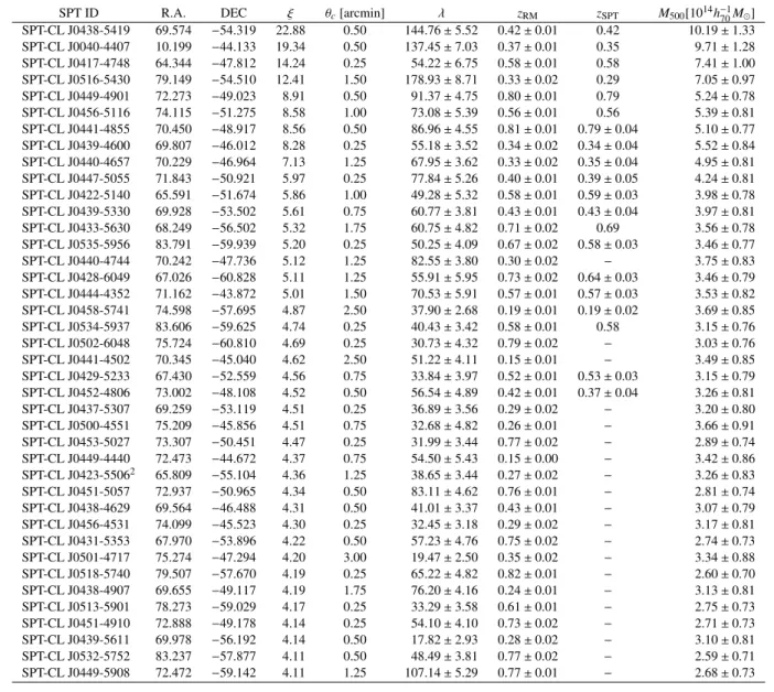
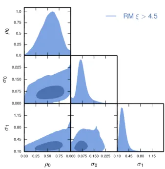
We marginalize over the SZE-mass scaling relation parameters and constrain the posterior distributions for the RM λ-mass scaling rela-tion. Our best fit parameters and 68% confidence level intervals are reported in Table 2 and shown in Figure 3. We note that the slope of the λ-mass relation is consistent with 1 within 1σ (consistent, therefore, with the richness being proportional to the mass), and the model is consistent with no redshift evolution within 1σ (An-dreon & Congdon 2014). Furthermore the resulting λ-mass relation is characterized by a remarkably low asymptotic intrinsic scatter, with σlnλ|M500 → 0.15− +0.10−0.07 as hlnλ|M500i → ∞ (Eq. 8). Following
Evrard et al. (2014), we estimate the characteristic scatter in mass at fixed richness to arrive at σln M = 0.18+0.08−0.05at λ = 70, ∼ 25%
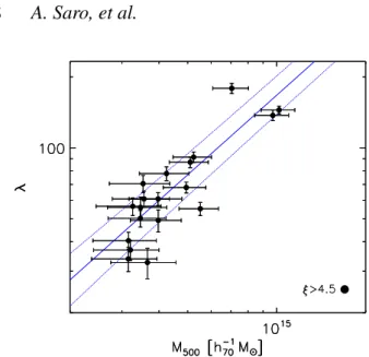
larger than the corresponding characteristic scatter in mass at fixed ξ. We present in Figure 4 the RM richness as a function of the SPT derived masses. Blue lines describe the best fitting model and in-trinsic scatter as derived from this analysis (Table 2) at a pivot point of z= 0.6.
We have verified that our results are not dominated by uncer-tainties in the SZE-mass scaling relation by fixing these parameters to their best fit values. Our results are only marginally improved in this case. Consequently, future analyses with larger samples are expected to considerably reduce the uncertainties of the recovered λ-mass scaling relation parameters.
In Figure 4, one cluster appears to be an obvious outlier: SPT-CL J0516-5435 (ξ = 12.4, λ = 178.9,M500=7.05×10¹⁴h−170M ).
SPT-CL J0516-5345 is a well-known merger that is elongated in a north-south direction in the plane of the sky with an X-ray mass estimate nearly a factor of two larger than the SZE mass estimate. This cluster was in fact the strongest outlier in the sample of 14
0.0 0.5 1.0 1.5 Bλ −2.0 −0.5 1.0 2.5 Cλ 43 55 67 79 Aλ 0.00 0.25 0.50 0.75 Dλ 0.0 0.5 1.0 1.5 Bλ −2.0−0.5 1.0 2.5 Cλ 0.0 0.25 0.5 0.75 1.0 Aλ 0.00 0.25 0.50 0.75 Dλ ξ >4.5 Rykoff et al. 2012
Figure 3. Posterior distribution for the four parameters of the λ-mass scal-ing relation (Equations 7 and 8). Predictions from the scalscal-ing relation of Rykoff et al. (2012) are shown as dashed black lines. Best fitting parame-ters and associated 1σ uncertainties appear in Table 2.
clusters in Andersson et al. (2011). High et al. (2012) made a weak lensing measurement of SPT-CL J0516-5345, and found that there was a significant offset between the brightest central galaxy (BCG) and the weak-lensing centre, consistent with the merger hypothe-sis. Additionally, High et al. (2012) found that the weak-lensing mass was in better agreement with the SZE-mass estimate than the X-ray mass estimate, at a level consistent with elongation observed in the plane of the sky. Therefore, SPT-CL J0516-5345 appears to be an outlier due to true intrinsic scatter in the observable-mass relations, so we leave it in our analysis. We note, however, that whether or not we include SPT-CL J0516-5345 in the fit has a sig-nificant impact on our results. Our best fit parameters shift from Bλ= 1.14+0.21−0.18and Dλ= 0.15+0.10−0.07with this cluster, to Bλ= 1.00+0.17−0.15
and Dλ = 0.05+0.07−0.03 when SPT-CL J0516-5345 is not included in
the fit. Whether SPT-CL J0516-5345 represents a rare event in a non-Gaussian tail in the distribution of richness of galaxy clusters or the recovered log-normal scatter obtained when cluster SPT-CL J0516-5349 is included is more correct will thus need to await fu-ture analyses with larger samples.
We convert the P(M500|λ) scaling relation derived by Rykoff
et al. (2012) using abundance matching and the SDSS maxBCG cluster-catalog (Koester et al. 2007) to a richness–mass relation so that we can compare it to our results (see also Evrard et al. 2014). The predictions from Rykoff et al. (2012) are shown as dashed lines in Figure 3 under the assumption of no redshift evolution in the richness–mass relation. We note that all parameters of our derived RM λ-mass scaling relation for SPT-selected clusters are consistent with the Rykoff et al. (2012) values.
We repeat these analyses extending the sample to include those with 4 < ξ < 4.5 and find similar results (Table 2). The largest difference is in the redshift evolution term which now has a best fit value Cλ= 1.71+0.63−0.57. While formally this difference does not
have large statistical significance (1.3σ), it is coming from a sam-ple that includes a large fraction of the same clusters, so it is likely
Figure 4. Richness as a function of the SPT derived masses for the calibra-tion sample used in this analysis (Seccalibra-tion 2.3). Blue lines show the best fit richness-mass relation and 1σ intrinsic scatter.
statistically significant. A larger redshift evolution term would im-ply that higher redshift RM clusters are less massive at fixed λ. At the same time the derived scatter is also larger.
Two of the clusters in the 4 < ξ < 4.5 range are compatible with false associations. Excluding the two matched clusters with the highest probability of random associations results in a ∼ 1σ shift in Bλ(from Bλ = 1.17 to Bλ = 1.04) and in a ∼ 0.5σ shift
in Cλ(from Cλ = 1.71 to Cλ = 1.42), while the other
parame-ters (Aλand Dλ) are almost unchanged. Interestingly, even though
we have increased the number of clusters in the SPT-SZ+RM sam-ple by 40%, the constraints on the scaling relation parameters are only mildly tighter. There are two reasons for this. First these lower signal-to-noise SPT-SZ clusters have larger fractional mass uncer-tainties in ξ (hξi−1 ∼ 0.23 and hξi−1 ∼ 0.13 respectively for the
4 < ξ < 4.5 and ξ > 4.5 samples). Second, the richnesses are also systematically lower, leading to a larger Poisson variance. Thus, each low ξ cluster has less constraining power than a high ξ cluster, reducing the impact of extending the sample to include the lower mass systems.
4.2 Consistency Test of Model
We also test the consistency of the adopted scaling relation model with the data by examining whether we are finding the expected number of matches with the correct distribution in richness. To do this, we focus on the SPT-E field, which at ∼ 124.6 deg2 is the largest contiguous region covered by the DES-SVA1 data. We carry out two different tests.
In the first test, we examine whether we are finding the ex-pected number of SZE-selected clusters and whether these clus-ters have the expected number of optical matches with the correct λ distribution. We generate 106 Monte Carlo realizations of
clus-ter samples extracted from the halo mass function above M500>
1013.5h−1
70M and assign richnesses λ and SPT-SZ significance ξ
us-ing the parameters we extract from our analysis of the real matched catalog. These Monte Carlo mocks are generated taking into ac-count the survey area as a function of redshift sampled by RM in the SPT-E field. We then apply the SZE selection–either ξ > 4.5 or ξ > 4–and measure the cumulative distribution in λ of the
SZE-selected samples. We then compare this to the same distribution in the real matched catalog.
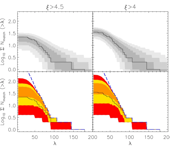
Shaded regions in the upper panels of Figure 5 show 1, 2, and 3σ confidence regions obtained from the mocks after marginalizing over the scaling relation parameters. The solid black line shows the distribution from the real catalog, which is in good agreement with the mocks. The largest observed difference is smaller than 1σ indi-cating that the adopted model provides a consistent description of the observed number and richness distribution of the SZE-selected sample. Similarly, a Kolmogorov-Smirnov (KS) test for the ob-served cumulative distribution of matched systems as a function of λ and the corresponding median distribution from the Monte Carlo simulations, shows that the null hypothesis of data being drawn from same distributions cannot be excluded and returns p−values 0.76 and 0.96 for ξ > 4.5 and ξ > 4, respectively.
The second test is focused on whether the RM cluster cata-log (which is significantly larger than the SPT-SZ catacata-log) has the expected number of SZE matches with the correct λ distribution. Essentially, we take the observed RM catalog as a starting point, and calculate the expected number of systems with SPT-SZ coun-terparts given the model and parameter constraints from our λ-mass likelihood analysis. This test differs from the first in that it takes the observedRM selected cluster sample as a starting point, and such a test should be more sensitive to, for example, contamination in the RM catalog. The formally correct way to evaluate a statistical difference between the RM selected sample and the SPT-SZ+RM matched sample used in this analysis would be to calibrate the λ-mass and SZE-λ-mass relations starting from the RM selected sam-ple. Such a study goes, however, beyond the scope of the current work and will be addressed in a future project. Therefore, the fol-lowing analysis is only intended to be a consistency check.
For this purpose, we proceed by first computing, for each real RM selected cluster in the SPT-E field, the probability Pmof that
cluster also having ξ > 4.5 and therefore being in the matched sample. We define this probability as:
Pm = Z ∞ 4.5 P(ξ|λ, z)dξ = Z ∞ 4.5 dξZ dM500P(ξ|M500)P(M500|λ, z), (10)
where P(M500|λ, z) ∝ P(λ|M500, z)P(M500, z) and P(M500, z) is the
halo mass function (Tinker et al. 2008).
To predict the expected number of RM clusters with SZE counterparts, we then randomly sample the scaling relation param-eters, determining Pm for all the RM clusters in each case. We
then Monte Carlo sample each Pmto produce randomly sampled
matched cluster catalogs. We use the results from the ensemble of random matched catalogs to produce the expected cumulative dis-tributions in λ. Orange, yellow, and red regions in the bottom panels of in Figure 5 show the 1, 2, and 3σ confidence regions, respec-tively, of the expected cumulative distribution in λ for ξ > 4.5 (left) and ξ > 4 (right), given the RM catalog and scaling relation param-eter constraints as input. The dashed blue line shows the cumulative distribution of the entire sample of RM clusters in the area, while the solid black line shows the observed cumulative distribution of the real matched catalog.
We note that the predicted number of SPT-SZ+RM matches in this case tends to be higher than that observed for λ > 35, but the tension is weak. Of some concern is the high λ end of the sample (λ > 70), where only 9 of the 17 RM selected clusters have SPT-SZ counterparts at ξ > 4.5 despite their having large probabilities indi-cating they should be in the SZE-selected sample. However, a KS
Figure 5. Consistency tests of our model (Section 3) and the SPT-SZ+RM catalog from the ∼124 deg2SPT-E field. The solid black lines show the observed
cumulative distribution in richness λ of the ξ > 4.5 (left) and ξ > 4 (right) SZE-selected samples. Upper panels: Gray scale regions show 1, 2, and 3σ regions predicted by drawing 106SZE-selected samples from the mass function and assigning λ according to our scaling relation constraints. There is good agreement
with the data. Lower panels: Dashed blue lines show the cumulative distribution in λ of the full RM sample. Orange, yellow, and red areas define 1, 2, and 3σ regions representing the predicted cumulative distribution of the SPT-SZ+RM catalog using as input the full RM sample and the probability (Eq. 10) that each RM cluster will have an SPT-SZ counterpart, given our scaling relation constraints.
test for the observed cumulative distribution of matched systems as a function of λ and the corresponding median distribution from the mocks shows that the null hypothesis of data being drawn from the same parent distribution cannot be excluded and returns p−values 0.90 and 0.33, respectively, for ξ > 4.5 and ξ > 4.
While the KS test is showing no evidence for the two distribu-tions to differ, it is also known to be not very sensitive to the tails of the distributions (Moscovich-Eiger et al. 2013). With this respect, it is also therefore interesting to directly compare the observed cu-mulative distribution with the cucu-mulative distribution from the pre-dicted number of matches. In this case, as for the classical KS test, we focus on the largest difference between the two distributions. Lower left panel of Figure 5 shows that at most, the observed cu-mulative distribution is in tension with expectations at the ∼ 2σ level, providing some indication of tension between the observed sample and our model. For example, when restricting ourselves to
clusters with λ > 70, we find that our simulation results in a larger number of SPT+RM associations in 94.6% of our Monte Carlo re-alizations. This tendency to observe fewer matches than expected given the size of the RM selected sample could be explained by ei-ther contamination within the RM sample, additional incomplete-ness within the SPT-SZ sample beyond that caused by scatter in the SZE-mass relation, or simply a statistical fluctuation. Future work exploring the SZE properties of the lower mass systems along with an extension of the current analysis to the full overlap between DES and the SPT-SZ survey will sharpen this test.
4.3 Optical-SZE Positional Offset Distribution
It has been shown that optical-miscentering can have a significant impact on the derived SZE signature for an optically-selected sam-ple (Biesiadzinski et al. 2012; Sehgal et al. 2013; Rozo & Rykoff
Figure 6. SPT-CL J0433-5630: DES-SVA1 gri pseudo colour image over-plotted with SPT-SZ signal-to-noise contours (in steps∆ξ=1). The magenta circle shows the projected R500/2 radius at z = 0.69, while the green circle
describes the 1σ SPT positional uncertainty (Eq.11). The cyan label marks the associated λ ∼ 60 RM cluster.
2014; Rozo et al. 2014a,b). We note, however, that in our case the SZE signal has been estimated at the SZE-determined position, so our results are not affected by optical miscentering. In fact, we can now use our data to constrain the distribution of offsets between the SZE-determined and the optically-determined cluster centres.
As an example, we show in Figure 6 the DES-SVA1 gri pseudo colour image of SPT-CL J0433-5630, an SPT-SZ selected cluster with ξ ∼ 5.3 at redshift z = 0.69 (B15). Yellow contours show the SPT-SZ signal-to-noise in steps of∆ξ = 1, while the ma-genta circle describes the projected radius R500/2. The cyan label
refers to the associated RM cluster centre. This RM cluster has rich-ness λ ∼ 60. We note that the most probable central galaxy selected by RM is significantly offset from the SZE defined centre. As a re-sult, the measured SZE signature at the optical position (ξ = 4.1) would be significantly underestimated with respect to the derived unbiased quantity ζ= 5 obtained through Eq. 3. We stress that this effect is not important for the scaling relation results reported in Section 4.1, as the sample analyzed here is SZE-selected.
Figure 7 contains a normalized histogram of the distribution of cluster positional offsets in units of R500for the ξ > 4.5 analyzed
SPT-SZ sample. Under the assumption that the measurement uncer-tainty from the optical side is negligible, we model this distribution as an underlying intrinsic positional offset distribution convolved with the SPT-SZ positional uncertainty.
The 1σ SPT-SZ positional uncertainty for a cluster with a pressure profile given by a spherical β model with β= 1 and core radius θc, detected with SPT-SZ significance ξ is described by:
∆θ = ξ−1qθ2
beam+ θ2c, (11)
where θbeam= 1.2 arcmin is the beam FWHM (see Story et al. 2011
and Song et al. 2012 for more details). As a result, the expected distribution of positional offsets in the case in which the intrinsic one is a δ−function is shown (arbitrarily rescaled) as a green line.
Song et al. (2012) have shown that the intrinsic optical-SZE positional offset distribution for an SPT-SZ selected sample is con-sistent with the optical−ray positional offset distribution of X-ray selected clusters (Lin et al. 2004). The offset distribution can be characterized by a large population of central galaxies with small
Figure 7. Solid histogram shows the measured fraction of SPT-SZ+RM clusters as a function of the optical-SZE positional offset in units of R500.
The green curve shows the SPT-SZ positional uncertainty, and the blue curves shows the best fitting SZE-optical positional offset model.
Table 3. Best fitting parameters and 68% confidence level of the optical-SZE positional offset distribution.
Catalog ρ0 σ0[R500] σ1[R500]
RM-ξ > 4.5 0.63+0.15−0.25 0.07+0.03−0.02 0.25+0.07−0.06
offsets from the SZE centres and a less populated tail of central galaxies with large offsets (e.g. Lin et al. 2004; Rozo & Rykoff 2014; Lauer et al. 2014). We therefore parametrize the distribution of positional offsets between the RM centre and the SZE centre for xas: P(x)= 2πx ρ0 2πσ2 0 e −x2 2σ20 +1 − ρ0 2πσ2 1 e −x2 2σ21 (12) where x= r/R500. While this model for the distribution was
mo-tivated by the expected intrinsic positional offset distribution, the measured distribution will include both the actual physical SZE-central galaxy offset distribution and the systematics due to fail-ures in identifying the correct cluster center with the RM algo-rithm. For every cluster and parameter ρ0 ∈ [0, 1], σ0 ∈ [0, 1],
and σ1 ∈ [σ0, 1], we then compare the predicted offset
distribu-tion obtained by convolving the model with the SPT-SZ posidistribu-tional uncertainty of Eq. 11 to extract the associated likelihood. Best fit parameters and 68% confidence intervals are shown in Table 3 and joint and fully marginalized parameter constraints are shown in Fig-ure 8.
We note that the positional offset distribution for the RM sam-ple is consistent with a concentrated dominant population (ρ0 =
0.63+0.15−0.25) of smaller offsets (σ0 = 0.07+0.03−0.02 R500) and a
sub-dominant population characterized by larger offsets (σ1= 0.25+0.07−0.06
R500). In the limit where the SZ center and BCG are coincident
for every cluster, the RM code(Rykoff et al. 2012, 2014) predicts the SZ-RM offset distribution for this sample to contain a centrally peaked component with normalization hPceni to be 0.79. While this
is formally consistant with the measured SZ - RM offset distri-bution, intrinsic optical-SZE positional offsets, such as those pre-sented by (e.g., Song et al. 2012) likely contribute to large
sepa-0.000 0.075 0.150 0.225 σ0 0.00 0.25 0.50 0.75 ρ0 0.10 0.45 0.80 1.15 σ1 0.000 0.075 0.150 0.225 σ0 0.0 0.25 0.5 0.75 1.0 ρ0 0.10 0.45 0.80 1.15 σ1 RM ξ > 4.5
Figure 8. Posterior distribution for the 1 and 2σ level of the three parame-ter model describing the positional offset distribution of Equation 12. Best fitting parameters are shown in Table 3.
ration component of the observed distribution shown in Figure 7. Larger samples will be necessary to disentangle the impact of sys-tematics due to failures in identifying the correct cluster centre with the RM algorithm from the offset distribution due to cluster mor-phology.
5 CONCLUSIONS
In this paper, we cross-match SZE-selected cluster candidates with ξ > 4.5 from the 2500d SPT-SZ survey (B15) with the optically-selected cluster catalog extracted from the DES science verifica-tion data DES-SVA1. The optically-selected catalog is created us-ing the RM cluster-findus-ing algorithm. We study the robustness of our matching algorithm by applying it to randomly generated RM catalogs.
Using the adopted matching algorithm in the 129.1 deg2 of
overlap between the two data sets, we create a matched catalog of 33 clusters. Eight of these clusters are removed as likely chance su-perpositions that are identified using the randomly generated cata-logs. The resulting 25 cluster sample includes all previously known z< 0.8 and ξ > 4.5 SPT-SZ clusters in this area (Song et al. 2012; Reichardt et al. 2013, B15) in addition to three previously uncon-firmed SPT-SZ clusters.
We then study three characteristics of this cross-matched SPT-SZ+RM cluster sample:
1) The richness mass relation of SPT-SZ selected clusters. We calibrate the λ-mass relation from SZE measurements by applying the method described in Bocquet et al. (2015). In this analysis we assume a fixed fiducial cosmology and marginalize over the simul-taneously calibrated SPT-SZ ξ-mass relation. We adopt flat priors on the richness–mass relation parameters. We find that the RM λ-mass relation for SPT-SZ selected clusters is characterized by a small asymptotic intrinsic scatter Dλ = 0.15+0.10−0.07 and by a slope
Bλ= 1.14+0.21−0.18that is consistent with unity. Our constraints are in
good agreement with those of Rykoff et al. (2012) and show that the scatter in mass at fixed richness λ= 70 for this sample is only 25% larger than the scatter in mass at fixed SPT-SZ observable ξ.
2) Consistency test of model and matched catalog. We carry out two consistency tests to determine whether there is tension be-tween the observed matched sample and the expectations given the scaling relation model we have adopted. Both tests involve creat-ing Monte Carlo generated cluster catalogs with associated richness and SPT-SZ significance derived from the fitted scaling relations. The first test checks whether the correct number of SZE-selected clusters is found and whether those clusters exhibit the correct num-ber of optical matches with the expected λ distribution. As is clear from Figure 5, the observations are perfectly consistent with the expectations from the model. Thus, our analysis shows that the data in our matched SPT-SZ+RM sample are well described by our adopted model. In the second test we take the much larger observed RM catalog as a starting point and use the model to test whether the expected number of SZE matches with the expected λ distribution is found. Unlike the first test, this one would in principle be sensi-tive to contamination within the RM sample. Here the agreement is not as good because there is a tendency for there to be fewer observed matches than expected. However, the tension reaches the ∼ 2σ level at worst, and so there is no convincing evidence that our observed sample is inconsistent with the model.
3) The SZE-optical positional offset distribution. We identify optical positional biases associated with 12% of the sample due to the masking in the DES-SVA1 data. We remove these clusters and study the optical-SZE positional offset distribution for the rest of the matched sample. We model the underlying positional offset distribution as the sum of two Gaussians, while accounting for the SPT-SZ positional uncertainty. We show that the resulting distri-bution is consistent with being described by a dominant (63+15−25%) centrally peaked distribution with (σ0 = 0.07+0.03−0.02R500) and a
sub-dominant (∼ 37%) population characterized by larger separations (σ1 = 0.25+0.07−0.06R500). For the same population, the RM algorithm
assumes that 79% of the clusters will belong to a small-offset pop-ulation, consistent with our observations.
We also match the SPT-SZ cluster candidates with 4 < ξ < 4.5 to the RM optical cluster catalogs from DES-SVA1 to extend the mass range of the SZE-selected clusters. Including the SPT-SZ can-didates between ξ= 4 and ξ = 4.5 increases the sample of matched clusters by ∼ 40% compared to the ξ > 4.5 sample, highlighting the potential synergies of SPT and DES in producing lower-mass ex-tensions of SZE-selected cluster samples. We show that this larger sample produces results that are broadly consistent with the ξ > 4.5 results, but only marginally tighter. This is due to the fact that mass constraints from lower signal-to-noise SPT clusters are somewhat weaker on a per cluster basis compared to the higher ξ sample. Fu-ture work benefiting from the larger region of overlap between the DES and SPT surveys will improve our derived constraints and help to better characterize the optical and SZE properties of cluster sam-ples in terms of positional offsets, purity, and completeness. More-over, the multiwavelength datasets available through DES and SPT enable characterization of the galaxy populations of large SZE-selected cluster samples, calibration of the SZE-SZE-selected cluster masses using weak lensing constraints, and many other promising studies.
ACKNOWLEDGEMENTS
We acknowledge the support by the DFG Cluster of Excellence ”Origin and Structure of the Universe”, the Transregio program TR33 ”The Dark Universe” and the Ludwig-Maximilians Univer-sity. The South Pole Telescope is supported by the National Science Foundation through grant PLR-1248097. Partial support is also provided by the NSF Physics Frontier Center grant PHY-1125897 to the Kavli Institute of Cosmological Physics at the University of Chicago, the Kavli Foundation and the Gordon and Betty Moore Foundation grant GBMF 947. A.A.S. acknowledges a Pell grant from the Smithsonian Institution. T. de Haan is supported by a Miller Research Fellowship. This work was partially completed at Fermilab, operated by Fermi Research Alliance, LLC under Con-tract No. De-AC02-07CH11359 with the United States Department of Energy.
REFERENCES
Abell G. O., 1958, ApJS, 3, 211 Aihara H. et al., 2011, ApJS, 193, 29
Allen S. W., Evrard A. E., Mantz A. B., 2011, ARAA, 49, 409 Andersson K. et al., 2011, ApJ, 738, 48
Andreon S., Congdon P., 2014, A&A, 568, A23 Annis J. et al., 2014, ApJ, 794, 120
Ascaso B., Wittman D., Dawson W., 2014, MNRAS, 439, 1980 Banerji M. et al., 2015, MNRAS, 446, 2523
Bartlett J. G., Silk J., 1994, ApJ, 423, 12 Benson B. A. et al., 2013, ApJ, 763, 147
Biesiadzinski T., McMahon J., Miller C. J., Nord B., Shaw L., 2012, ApJ, 757, 1
Bleem L. E., Stalder B., Brodwin M., Busha M. T., Gladders M. D., High F. W., Rest A., Wechsler R. H., 2015a, ApJS, 216, 20
Bleem L. E. et al., 2015b, ApJS, 216, 27 Bocquet S. et al., 2015, ApJ, 799, 214 B¨ohringer H. et al., 2000, ApJS, 129, 435 Borgani S. et al., 2001, ApJ, 561, 13
Cavaliere A., Fusco-Femiano R., 1976, A&A, 49, 137
Crawford T. M., Switzer E. R., Holzapfel W. L., Reichardt C. L., Marrone D. P., Vieira J. D., 2010, ApJ, 718, 513
de Jong J. T. A., Verdoes Kleijn G. A., Kuijken K. H., Valentijn E. A., 2013, Experimental Astronomy, 35, 25
Desai S. et al., 2012, ApJ, 757, 83
Diehl T. et al., 2012, Physics Procedia, 37, 1332 Eisenhardt P. R. M. et al., 2008, ApJ, 684, 905
Eke V. R., Cole S., Frenk C. S., Patrick Henry J., 1998, MNRAS, 298, 1145
Evrard A. E., Arnault P., Huterer D., Farahi A., 2014, MNRAS, 441, 3562
Flaugher B. et al., 2015, ArXiv e-prints:1504.02900
Flaugher B. L. et al., 2012, in Society of Photo-Optical Instrumen-tation Engineers (SPIE) Conference Series, Vol. 8446, Society of Photo-Optical Instrumentation Engineers (SPIE) Conference Series, p. 11
Gioia I. M., Maccacaro T., Schild R. E., Wolter A., Stocke J. T., Morris S. L., Henry J. P., 1990, ApJS, 72, 567
Gladders M. D., Yee H. K. C., 2000, AJ, 120, 2148 Haehnelt M. G., Tegmark M., 1996, MNRAS, 279, 545+ Hao J. et al., 2010, ApJS, 191, 254
Hasselfield M. et al., 2013, JCAP, 7, 8
High F. W. et al., 2012, ApJ, 758, 68 Koester B. P. et al., 2007, ApJ, 660, 239
Lauer T. R., Postman M., Strauss M. A., Graves G. J., Chisari N. E., 2014, ApJ, 797, 82
Laureijs R. et al., 2011, ArXiv e-prints:1110.3193 Lin Y., Mohr J. J., Stanford S. A., 2004, ApJ, 610, 745 Liu J. et al., 2015, MNRAS, 448, 2085
LSST Dark Energy Science Collaboration, 2012, ArXiv e-prints:1211.0310
Mantz A., Allen S. W., Ebeling H., Rapetti D., Drlica-Wagner A., 2010, MNRAS, 406, 1773
Mei S. et al., 2009, ApJ, 690, 42
Melchior P. et al., 2015, MNRAS, 449, 2219
Melin J.-B., Bartlett J. G., Delabrouille J., 2006, A&A, 459, 341 Menanteau F. et al., 2010, ApJS, 191, 340
Mohr J. J. et al., 2008, in Society of Photo-Optical Instrumen-tation Engineers (SPIE) Conference Series, Vol. 7016, Society of Photo-Optical Instrumentation Engineers (SPIE) Conference Series
Mohr J. J. et al., 2012, in Society of Photo-Optical Instrumen-tation Engineers (SPIE) Conference Series, Vol. 8451, Society of Photo-Optical Instrumentation Engineers (SPIE) Conference Series, p. 0
Moscovich-Eiger A., Nadler B., Spiegelman C., 2013, ArXiv e-prints
Muzzin A. et al., 2012, ApJ, 746, 188
Ngeow C. et al., 2006, in Society of Photo-Optical Instrumenta-tion Engineers (SPIE) Conference Series, Vol. 6270, Society of Photo-Optical Instrumentation Engineers (SPIE) Conference Se-ries
Pacaud F. et al., 2007, MNRAS, 382, 1289 Planck Collaboration et al., 2015, ArXiv e-prints Reichardt C. L. et al., 2013, ApJ, 763, 127
Rozo E., Bartlett J. G., Evrard A. E., Rykoff E. S., 2014a, MN-RAS, 438, 78
Rozo E., Evrard A. E., Rykoff E. S., Bartlett J. G., 2014b, MN-RAS, 438, 62
Rozo E., Rykoff E. S., 2014, ApJ, 783, 80
Rozo E., Rykoff E. S., Bartlett J. G., Melin J. B., 2014c, ArXiv e-prints
Rozo E. et al., 2010, ApJ, 708, 645 Rozo et al., 2015, In Preparation Rykoff E. S. et al., 2012, ApJ, 746, 178 Rykoff E. S. et al., 2014, ApJ, 785, 104 Rykoff et al., 2015, In Preparation
S´anchez C. et al., 2014, MNRAS, 445, 1482 Sehgal N. et al., 2013, ApJ, 767, 38 Soares-Santos M. et al., 2011, ApJ, 727, 45 Song J. et al., 2012, ApJ, 761, 22
Staniszewski Z. et al., 2009, ApJ, 701, 32 Story K. et al., 2011, ApJ, 735, L36+
Sunyaev R. A., Zel’dovich Y. B., 1972, Comments on Astro-physics and Space Physics, 4, 173
The Dark Energy Survey Collaboration, 2005, ArXiv Astro-physics e-prints
Tinker J., Kravtsov A. V., Klypin A., Abazajian K., Warren M., Yepes G., Gottl¨ober S., Holz D. E., 2008, ApJ, 688, 709 ˇSuhada R. et al., 2012, A&A, 537, A39
Vanderlinde K. et al., 2010, ApJ, 722, 1180 Viana P., Liddle A., 1999, MNRAS, 303, 535 Vikhlinin A. et al., 2009, ApJ, 692, 1060
Vikhlinin A., McNamara B., Forman W., Jones C., Quintana H., Hornstrup A., 1998, ApJ, 502, 558
Wen Z. L., Han J. L., Liu F. S., 2012, ApJS, 199, 34
White S. D. M., Efstathiou G., Frenk C. S., 1993, MNRAS, 262, 1023
Wiesner M. P., Lin H., Soares-Santos M., 2015, ArXiv e-prints Zenteno A. et al., 2011, ApJ, 734, 3
Zwicky F., Herzog E., Wild P., 1968, Catalogue of galaxies and of clusters of galaxies. California Institute of Technology, Pasadena
1Department of Physics, Ludwig-Maximilians-Universitaet,
Scheinerstr. 1, 81679 Muenchen, Germany
2Excellence Cluster Universe, Boltzmannstr. 2, 85748 Garching,
Germany
3Department of Physics, University of Arizona, 1118 E 4th St,
Tucson, AZ 85721
4Fermi National Accelerator Laboratory, P. O. Box 500, Batavia,
IL 60510, USA
5Kavli Institute for Cosmological Physics, University of Chicago,
Chicago, IL 60637, USA
6Department of Astronomy and Astrophysics,University of
Chicago, 5640 South Ellis Avenue, Chicago, IL 60637
7Max Planck Institute for Extraterrestrial Physics,
Giessenbach-strasse, 85748 Garching, Germany
8Kavli Institute for Particle Astrophysics& Cosmology, P. O. Box
2450, Stanford University, Stanford, CA 94305, USA
9SLAC National Accelerator Laboratory, Menlo Park, CA 94025,
USA
10Argonne National Laboratory, 9700 South Cass Avenue, Lemont,
IL 60439, USA
11Center for Cosmology and Astro-Particle Physics, The Ohio
State University, Columbus, OH 43210, USA
12Department of Physics, The Ohio State University, Columbus,
OH 43210, USA
13Laborat´orio Interinstitucional de e-Astronomia - LIneA, Rua
Gal. Jos´e Cristino 77, Rio de Janeiro, RJ - 20921-400, Brazil
14CERN, CH-1211 Geneva 23, Switzerland
15Universit¨ats-Sternwarte, Fakult¨at f¨ur Physik,
Ludwig-Maximilians Universit¨at M¨unchen, Scheinerstr. 1, 81679 M¨unchen, Germany
16Cerro Tololo Inter-American Observatory, National Optical
Astronomy Observatory, Casilla 603, La Serena, Chile
17Department of Physics& Astronomy, University College London,
Gower Street, London, WC1E 6BT, UK
18Department of Physics and Astronomy, University of
Pennsylva-nia, Philadelphia, PA 19104, USA
19Institute of Astronomy, University of Cambridge, Madingley
Road, Cambridge CB3 0HA, UK
20Institut de Ci`encies de l’Espai, IEEC-CSIC, Campus UAB,
Fac-ultat de Ci`encies, Torre C5 par-2, 08193 Bellaterra, Barcelona, Spain
21Department of Physics, Harvard University, 17 Oxford Street,
Cambridge, MA 02138
22Harvard-Smithsonian Center for Astrophysics, 60 Garden Street,
Cambridge, MA 02138
23Institut d’Astrophysique de Paris, Univ. Pierre et Marie Curie&
CNRS UMR7095, F-75014 Paris, France
24Department of Physics and Astronomy, University of Missouri,
5110 Rockhill Road, Kansas City, MO 64110
25Department of Physics and Enrico Fermi Institute, University of
Chicago, 5640 South Ellis Avenue, Chicago, IL 60637
26Institute of Cosmology& Gravitation, University of Portsmouth,
Portsmouth, PO1 3FX, UK
27Observat´orio Nacional, Rua Gal. Jos´e Cristino 77, Rio de
Janeiro, RJ - 20921-400, Brazil
28Department of Astronomy, University of Illinois,1002 W. Green
Street, Urbana, IL 61801, USA
29National Center for Supercomputing Applications, 1205 West
Clark St., Urbana, IL 61801, USA
30George P. and Cynthia Woods Mitchell Institute for Fundamental
Physics and Astronomy, and Department of Physics and Astron-omy, Texas A&M University, College Station, TX 77843, USA
31Department of Physics, McGill University, 3600 Rue University,
Montreal, Quebec H3A 2T8, Canada
32Department of Physics, University of California, Berkeley, CA
94720
33Jet Propulsion Laboratory, California Institute of Technology,
4800 Oak Grove Dr., Pasadena, CA 91109, USA
34Department of Astronomy, University of Michigan, Ann Arbor,
MI 48109, USA
35Department of Physics, University of Michigan, Ann Arbor, MI
48109, USA
36Institut de F´ısica d’Altes Energies, Universitat Aut`onoma de
Barcelona, E-08193 Bellaterra, Barcelona, Spain
37Australian Astronomical Observatory, North Ryde, NSW 2113,
Australia
38Department of Astronomy, The Ohio State University, Columbus,
OH 43210, USA
39Kavli Institute for Astrophysics and Space Research,
Mas-sachusetts Institute of Technology, 77 MasMas-sachusetts Avenue, Cambridge, MA 02139
40Brookhaven National Laboratory, Bldg 510, Upton, NY 11973,
USA
41School of Physics, University of Melbourne, Parkville, VIC 3010,
Australia
42Department of Physics and Astronomy, Pevensey Building,
University of Sussex, Brighton, BN1 9QH, UK
43Centro de Investigaciones Energ´eticas, Medioambientales y
Tecnol´ogicas (CIEMAT), Madrid, Spain
44Institute for Astronomy, University of Hawaii at Manoa,
Hon-olulu, HI 96822, USA
45Department of Physics, University of Illinois, 1110 W. Green St.,
Urbana, IL 61801, USA
46Department of Physics, Stanford University, 382 Via Pueblo
Mall, Stanford, CA 94305
47Cerro Tololo Inter-American Observatory, Casilla 603, La
Serena, Chile
APPENDIX A: STUDY OF MASS-RICHNESS SCATTER FOR CLUSTERS FOUND WITH THE VT METHOD The scatter of the mass-richness relation is a primary source of sys-tematic uncertainties in cosmological measurements using galaxy clusters. To ensure that this and other astrophysical systematics are kept under control in future cosmology analyses, the DES collabo-ration has pursued the development of multiple cluster finding al-gorithms. Here we present initial results obtained using the analysis framework described throughout this paper on a DES-SVA1 cluster catalog created using the Voronoi Tessellation (VT) cluster finder (Soares-Santos et al. 2011). The VT method is fundamentally dif-ferent from RM. Specifically, VT uses photometric redshifts to de-tect clusters in 2+1 dimensions, and is designed to produce a cluster catalog up to z ∼ 1 and down to mass M ∼ 1013.5M