A cumulus ensemble model with simple mesoscale structure

A CUMULUS ENSEMBLE MODEL WITH SIMPLE MESOSCALE STRUCTURE

by

GEORGE JOHN HUFFMAN

B.S., The Ohio State University, 1976

SUBMITTED TO THE DEPARTMENT OF METEOROLOGY AND PHYSICAL OCEANOGRAPHY IN PARTIAL FULFILLMENT

OF THE REQUIREMENTS FOR THE DEGREE OF DOCTOR OF PHILOSOPHY

at the

O MASSACHUSETTS INSTITUTE OF TECHNOLOGY

January, 1982

Signature of Author

Certified by

Accepted by

Department of Meteorology and Physical Oceanography 8 January 1982

2/

Frederick Sanders Thesis Supervisor

Peter H. Stone Chairman, Departmental Committee on Graduate Students

LUndgren

. -i",--,0 L _J.98 2

...

'"D

o ,.

A CUMULUS ENSEMBLE MODEL WITH SIMPLE MESOSCALE STRUCTURE by

GEORGE JOHN HUFFMAN

Submitted to the Department of Meteorology and Physical Oceanography on 8 January 1982 in partial fulfillment of the requirements for the degree of Doctor of Philosophy Abstract

In this study we consider the transport and release of heat and mois-ture by a cumulus cloud ensemble, including an examination of the role which mesoscale organization plays in the ensemble's activities. A

numerical model is constructed and the results of the model are compared with observations.

Observations reveal that many properties of cumulus ensembles are lognormally distributed over the ensemble. Mesoscale structure is fre-quently observed, often as clumps of cumuli with or without other organ-ization. The largest, longest-lasting clouds producing the most rain tend to be found in mesoscale clumps. Residual budget calculations from large scale observation show warming and drying at nearly all lev-els, although the details depend on geographic location.

A new cumulus ensemble model is developed. First, a time-dependent, axisymmetric, anelastic cumulus cloud model is formulated after Asai and Kasahara (1967) and Yau (1980), but with a careful analysis of lateral entrainment. This analysis shows no horizontal scale dependence due to entrainment; scale dependence arises instead from the pressure perturba-tion associated with the cumulus cloud. Other tests show that the Kes-sler (1969) microphysical parameterization yields the largest errors at cloud top and below cloud base.

This individual cumulus cloud model is generalized to a time-depen-dent cumulus ensemble model with tophat variable profiles in each model region. The numbers of clouds in different size classes are free parameters, determined by requiring that the model simulate the domain-averaged subcloud moisture budget. The mesoscale feature is assumed to contain all cumulus clouds.

Starting at 00Z on Day 245 of GATE, the cumulus ensemble model pre-dicts minimal cloud activity until the sounding becomes more unstable than the initial sounding. The amount of destabilization required depends only weakly on the cloud size distribution chosen. Members of the ensemble tend to be either shallow/weak or deep/vigorous: There are relatively few middle-sized clouds. The mesoscale version produces more vigorous convection. Mesoscale contributions are shown to be important in the budgets of heat, moisture, and mass. A mesoscale anvil forms only after the outer environment saturates.

Title: Professor of Meteorology Acknowledgements and Dedication

I wish to thank Dr. David Randall and Professor Frederick Sanders for serving as my advisors during the course of this thesis. Early work on

this thesis was carried out under Dr. Randall, who continued to maintain an active interest after moving to the NASA GLAS. The thesis was com-pleted under Professor Sanders. Their diverse insights into the prob-lem at hand and meteorology in general had a significant effect on my studies at MIT. I also wish to thank the members of the MIT Convection Club for helpful suggestions, particularly Frank Colby and Brad Colman, who read early drafts of the thesis.

Several sources of assistance made this project possible. Funding was provided by NSF grants 79-10844 ATM and 80-19301 ATM. The NASA Goddard Laboratory for Atmospheric Sciences provided the computer time required to develop and run the thesis model and to prepare the thesis. Diana L. Spiegel, site manager of the Department of Meteorology and Physical Oceanography's computer facility, provided unstinting assis-tance in dealing with the computer. Prof. Man-Kong Yau of McGill Uni-versity provided an early version of the one-cloud model. The GATE data for model initialization and budget comparison were processed by a group at the University of Washington under Prof. Richard Reed. The thesis was printed at NASA GSFC assistance of James Abeles. Figures were expertly prepared by Isabelle Kole (line drawings) and Frank Colby (pho-tographs).

A special acknowledgement is due Randy Dole, with whom I shared an office during this thesis. He was a ready source of encouragement and consultation throughout our striving towards our respective graduations. I am also grateful to the congregation of Old West Church for encourage-ment and a sense of perspective. Finally, I wish to dedicate this the-sis to my parents, for their concern and understanding over the years.

Table of Contents

Page Title . . . . . . . . . . . . . . .

Abstract . . . . . . . . . . . . . . Acknowledgements and Dedication . .

Table of Contents . . . . . . . . . Figure Legends . . . . . . . . . . . Table Legends . . . . . . . . . . . Chapter 1: Introduction ... Chapter 2: Observations . . . . . . 2.1 Introduction . . . . 2.2 Cumulus ensembles 2.3 Mesoscale structure 2.4 Residual calculations 2.5 Summary . . . . . . Chapter 3: Cumulus Ensemble Models

3.1 Introduction . . . . 3.2 Models with explicit

Chapter 4:

Chapter 5:

3.3 Models with parameter

3.4 Cloud-environment int

3.5 Summary

The Model: One Cloud .

4.1 General design . . . 4.2 Preliminary remarks horizontal str ized horizonta eractions . ._{. . . . . .} . . . . . . . . . . . . . . . . . . . . . . . . . . . . . . . . . . . . horizontal str ized horizonta eractions . . . . . . . . . . . . . . 4.3 Entrainment and the conservation laws 4.4 Application to a two-cylinder model 4.5 The complete cloud model .. ... 4.6 Cloud model behavior and sensitivity 4.7 Summary . . . . . . . . . . . . . . The Model: Ensemble . . . . . . . . . .

5.1 Introduction . . . . . . . . . . . .

5.2 Many clouds in a common environment 5.3 Including mesoscale organization . .

5.4 Additional details . . . . . . . . . 5.5Summary ... . . . . . . . . . . . . . . . . . . . . . . . . . . . . . . . . . uct l . . . . . . . . . . . . . . . . . . . . . . . . . . . . . . . . . . . . . . . . . . . . ure .. tructure . . . . . . . . . . . . . . . . . . . . . . . . . . . . . . . . . . . . . . . . . . . . . . . . . . . . . . . . . . . . . . . . 1 2 3 4

6

56

63

66

96

98

98

98

101

105

111

Chapter 6: Model Results . . . . . . . . . . . . . . . . . .

6.1 Introduction ...

6.2 Observations of Day 245 . . . . . . . . . . . .

6.3

6.4 A case with mesoscale structure . . . . . . . .

6.5 Test of varying mesoscale region cloud coverage

. &... 180

6.6 Test of varying cloud distribution . 6.7 Test of increasing the allowed range

radii . . . . . . . . . . . . . . 6.8 Test of starting 3 hr earlier . . . 6.9 Summary . . . . . . . . . . . . . . Summary and Concluding Remarks . . . . . Symbols . . . . . . . . . . . . . . . . A Stochastic Model of Cumulus Clumping B.1 Introduction . . . . . . . . . . . B.2 Model formulation . . . . . . . . . B.3 Results . . . . . . . . . . . . . . B.4 The stabilization profile . . . . . B.5 Discussion and conclusions .

A Two-Cylinder Cloud Model . . . . . . C.1 Introduction . . . . . . . . . . . C.2 Model equations . . . . . . . . . . C.3 Microphysical parameterizations . . C.4 Perturbation pressure treatment . .

C.5 Computational considerations . . . . . . 187 of cloud 197 202 209 ... 211 . . . 217 . . . 220 220 221 223 230 232 234 234 234 236 237 243 GATE Data Analysis . . . . . . . .

D.1 Introduction . . . . . . . . .

D.2 Soundings and budgets . . . . .

D.3 Radiative transfer . . . . . . D.4 Precipitation . . . . . . . . . Budget Derivation . . . . . . . . . References . . . . . . . . . . . . . . . . . . . Biographical Note . . . . . . . . . . . . . . . . . . . . . 245

245

245

246

249

118

Figure Legends

Figure Page

2.1 Variation with altitude of 50 percentile (o) and 10 percentile (A) up- and downdraft cores, with respect to core diameter, mean vertical velocity of cores, maximum 1 s vertical velocity

within core, and core mass flux. (LeMone and Zipser, 1980,

Fig. 5) .. .. .... . . . . .. . .. * ... . 19 2.2 Mean vertical velocity in up- and downdraft cores as a

func-tion of height. GATE data for 50 percentile (o) and

10 percentile (A) cores from LeMone and Zipser (1980), Fig. 5;

Thunderstorm Project data adopted from Byers and Braham

(1949), Tables 7 and 10; for the 4.5 km level only, hurricane

data from Gray (1965), Fig. 13 (.,A). (Zipser and LeMone,

1980, Fig. 1) .. .. ... ... . . . ... . . 19

2.3 Mean "cloud"-average updraft and maximum up- and downdraft speeds as a function of height from GATE (dashed) and eastern Australia (solid). GATE values approximated from LeMone and Zipser (1980), Figs. 4b-c for cores; Australia values from

Warner (1970). . . . . ... 21

2.4 Cumulative frequency distribution of (a) maximum area,

(b) lifetime, (c) total rainfall, in log-probability coordi-nates for the cells of composite echoes (groups) and for sin-gle-cell echoes (individual) in GATE. (L6pez, 1978, Figs. 6,

7, 8) ...* . * .* o ... * . 26

2.5 (a) Duration, (b) average rainfall, (c) total rain as a

func-tion of average area for the cells of composite echoes

(groups) and for single-cell echoes (individual) in GATE.

(L6pez, 1978, Figs. 9, 10, 11) . . .... ... . 27

2.6 Vertical profiles of the apparent sensible heat source (Q,)

and apparent latent heat sink (Q.) for the B-scale area in GATE (E. ATL) and the Marshall Islands (W. PACIFIC). (after

Thompson et al., 1979, Fig. 8) . ... . . ... . 31

3.1 Temperature (T) and dewpoint (Td) soundings taken from the

ship Researcher at 00Z 12 August 1974. Dotted line is a

moist adiabat. (after Soong and Tao, 1980, Fig. 5) . ... . . 37 3.2 Computed w at 3 h intervals within the ITCZ rainband during

00-24Z 12 August 1974. (Soong and Tao, 1980, Fig. 3) . . . . 38

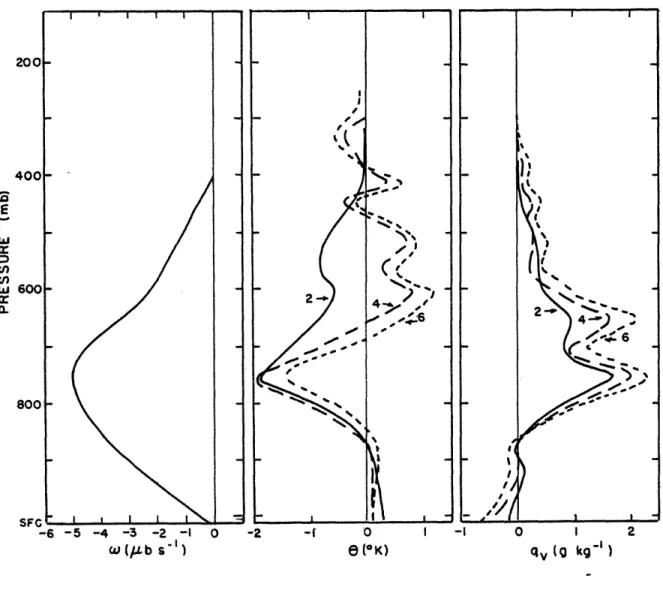
3.3 Domain-averaged cloud heating and moistening effects

(sub-scripted c) for each 6 h during 00-24Z 12 August 1974 simu-lated by Soong and Tao (1980, "ST"), with the corresponding

observed Q,-Qi and -(cp/L)Q 2. (ST, Fig. 19) ... . 38

Figure Page 2 h interval using the w profile as simulated by Soong and Tao (1980, "ST"). (ST, Fig. 20) . ... 40

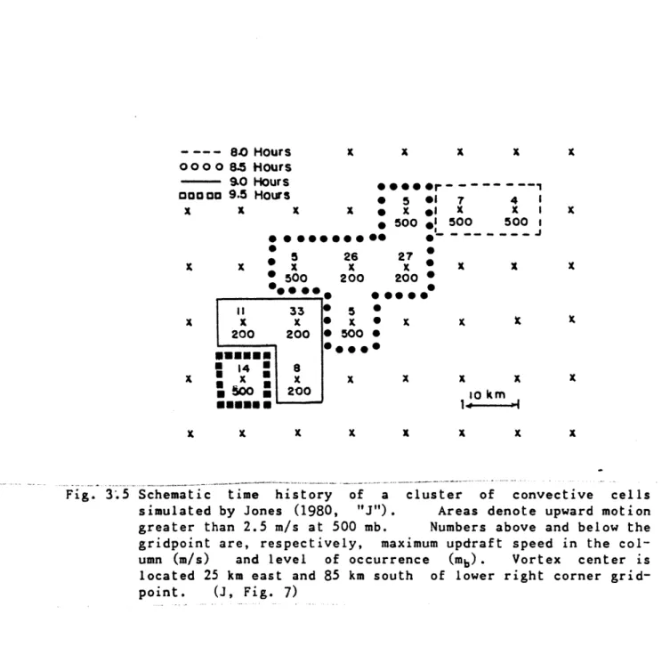
3.5 Schematic time history of a cluster of convective cells simu-lated by Jones (1980, "J"). Areas denote upward motion greater than 2.5 m/s at 500 mb. Numbers above and below the gridpoint are, respectively, maximum updraft speed in the col-umn (m/s) and level of occurrence (mb). Vortex center is located 25 km east and 85 km south of lower right corner grid-point. (J, Fig. 7) . ... . . .. ... 42 3.6 "Peak" and "dip" stabilization profiles tested by Randall and

Huffman (1980, "RH"). The two curves have the same area-av-eraged values (over the disk). The constant stabilization case is shown for reference only. (RH, Fig. 1) ... 44 3.7 Environmental mass flux (), mean mass flux (-), and net

con-vective-mesoscale mass flux (HM+Md,), for category 4 of the Reed et al. (1977) wave for Johnson's (1980, "J") spectral diagnostic models with convective updrafts alone, convective up- and downdrafts, and convective up- and downdrafts plus mesoscale downdrafts. (J, Fig. 18) . ... 47 4.1 Schematic diagram depicting the "pie-slice" of cloud over

which integration is performed to obtain (4.2). . ... 59 4.2 Initial temperature (T) and dewpoint (Td) soundings used in

Chapter 4. . ... . . . . . 72 4.3 Detailed time-height plots of area-averaged inner cylinder

variables for Version P: Wa, vertical velocity (m/s, val-ues < -1 m/s shaded); SO', , deviation from initial potential

temperature profile (OC); qea, cloud water mixing ratio (g/kg); qr, rain water mixing ratio (g/kg). Heavy dashed line at 35 min is the 20% cutoff point (see Section 4.6). . . 73

4.4 Microphysical parameterization comparison. Version P,

(a) moistening, and (b) heating; Version K, (c) moistening, and (d) heating. The net change (--) is the sum of net ver-tical transports, both cloud-scale (-+-) and turbulent (-X-), condensational heating/drying (- -), and evaporative cooling/ moistening, both cloud (-o-) and rain (-*-) evaporation. (e)

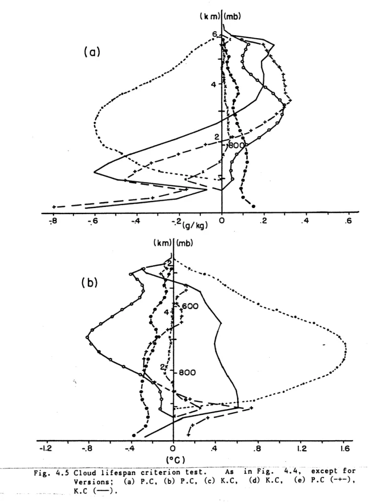
Inner cylinder up- and downdraft mass fluxes for P (-+-) and K (-- ). . . . . . . . . . . . . . . . . . . . . . . . . . . . . 79 4.5 Cloud lifespan criterion test. As in Fig. 4.4, except for

Versions; (a) P.C, (b) P.C, (c) K.C, (d) K.C, (e) P.C (-+-), K.C (-- ) . . . . . . . . . . * . . .. . . 85

4.6 Horizontal rain advection test. As in Fig 4.4, except for Versions; (a) P.R, (b) P.R, (c) K.R, (d) K.R, (e) P.R (-+-),

Figure Page K.R (-)... . . ... . . .. . * * * ... 88

4.7 Vertical resolution test. As in Fig. 4.4, except for Ver-sions; (a) K.G, (b) K.G; and (c) as in Fig. 4.4e, except K.G

(-- ). . . . . . 92

4.8 Large-scale lifting test. As in Fig. 4.4, except for Ver-sions; (a) K.W, (b) K.W, and (c) as in Fig. 4.4e, except K.W (-). Large-scale moistening, heating, and mass flux are shown as dotted lines. . ... ... 94 5.1 Schematic representation of a cumulus cloud ensemble.

(a) Clouds in a homogeneous large-scale environment (bounded

by E). (b) A system containing clouds, a mesoscale feature (bounded by M), and an outer environment (bounded by E). A cross section (C-C') is shown in Fig. 5.2. ... 100

5.2 Schematic vertical cross section through Fig. 5.1b, showing some atmospheric levels and the maximum sizes clouds attain over their lifecycles. Level 4 is depicted as carrying a mesoscale anvil (not shown in Fig. 5.1b). E and M are the boundaries in Fig. 5.1b. . ... .... . 103 6.1 (a) 700 mb and (b) surface maps, including streamlines at 12Z

Day 245 over the GATE region. . ... ... . . 116

6.2 Infrared satellite picture (4x4 km) at (a) 00Z Day 245 and (b) 00Z Day 246 over the GATE region. . ... . 116 6.3 Estimates of precipitation on Day 245; (-.-) radar-derived

over the "Master Array", a circle circumscribing the B Array (Hudlow and Patterson, 1978); (-) heat budget-derived over the A/B Array (after Frank, 1979). . .. . . .. ... . 117

6.4 (a) Large scale vertical mass flux averaged over 3 hr inter-vals, (b) temperature and water vapor changes from initial state at 3 hr intervals due to all prescribed forcings, and (c) observed temperature and moisture changes from initial state at the end of each period. All data from Thompson et al. (1979). . ... . . . . ... .. 119 6.5 Temperature (T) and dewpoint (Td) soundings averaged over the

GATE B Array at 00Z Day 245. . ... . 123 6.6 Cumulative frequency distribution for Cases in Chapter 6;

(-.-) LN1, (-X-) LN2, (-+-) LN3, (-o-) AIC. ... 124 6.7 Maximum upward vertical velocity in the cloud column, and

sur-face rainfall rate at 2 min intervals over (a) 0-3 hr, (b)

3-6 hr, (c) 6-9 hr; Case LN1.NOM. ( o ) 0.50 km, ( + ) 0.78 km, (.--) 1.23 km, (---) 1.92 km, (-) 3.00 km radius

Figure Page clouds. . . . .. . . . . . . . . . . . . . . . . 125 6.8 Heat and moisture budgets over (a) 0-3 hr, (b) 3-6 hr, (c)

6-9 hr; Case LN1.NOM. Observed and simulated budgets are solid and dashed lines, respectively . ... ... . 129 6.9 Domain-averaged temperature and moisture changes.from initial

state at 3 hr intervals; Case LN1.NOM. . ... . . . 133 6.10 Individual subensemble and region contributions to (a) heat,

and (b) moisture budgets; Case LN1.NOM. ... 137

6.11 Vertical mass fluxes in cloud updrafts (MH), cloud downdrafts (M), clouds (Mc), and the environment (A) over (a) 0-3 hr, (b) 3-6 hr, (c) 6-9 hr; Case LN1.NOM. ... . . 140 6.12 Time-height plot of vertical velocity in the mesoscale region

over 6-9 hr; Case LN1.M20 ... . . ... 146 6.13 As in 6.8 for Case LN1.M20. . ... . ... 148 6.14 As in 6.9 for Case LN1.M20. . ... ... 151 6.15 As in 6.9 for Case LN1.M20, except for (a) outer

environment-averaged, and (b) mesoscale region-averaged. . ... . 153

6.16 As in 6.11 for Case LN1.M20, with vertical mass flux in the mesoscale region (M,). . ... . .. ... 155 6.17 Schematic diagram illustrating LeMone and Zipser (1980) flight

paths. ECS is Effective Cross Section of a cloud (measured perpendicular to a flight path). Path A shows a flight sam-pling a large cloud, missing a smaller cloud. Path B shows a flight with an in-cloud path length > 0.5 km. Path C shows a flight with in-cloud path length < 0.5 km (even though cloud diameter > 0.5 km) . ... . . . . 159 6.18 Up- and downdraft average vertical velocity 50 percentile (o)

and 10 percentile (A) speeds as a function of height. Solid symbols are LeMone and Zipser's (1980) GATE air-craft samples of "cores". All other data are for Case LNl.M20 over 6-9 hr, processed as in Section 6.4. Lines are level-by-level values, isolated symbols are layer averages, plotted at event-weighted heights. . ... . 161

6.19 Subensemble and region contributions to vertical mass flux; Case LN1.M20. . ... . . . . . . 164 6.20 Accelerations in the mesoscale region vertical velocity

equa-tion, averaged over 6-9 hr for Case LN1.M20, (a) with and (b) without vertical perturbation pressure gradient in the

Figure Page

mesoscale region. ... ... . . . . . . . . . . . . 165

6.21 Vertical mass flux in the mesoscale region, averaged over 6-9 hr for Case LN1.M20, with and without vertical perturba-tion pressure gradient in the mesoscale region. . ... . 169

6.22 As in Fig. 6.10 for Case LN1.M20 . ... . . . . . 171

6.23 Subensemble and region contributions to the heat and moisture budgets over 6-9 hr for Case LN1.M20 for various processes; (a) net condensation, (b) vertical eddy heat flux convergence, (c) vertical eddy vapor flux convergence, (d) vertical turbu-lent heat flux convergence, (e) vertical turbuturbu-lent vapor flux convergence (see Appendix E for formulae). . ... . 173

6.24 As in Fig. 6.8 for Case LN1.M10. . ... . . . . 181

6.25 AS in Fig. 6.8 for Case LN1.M30. . ... . . . . . 184

6.26 As in Fig. 6.9 for Case LN2.M20. . ... ... . 188

6.27 As in Fig. 6.8 for Case AIC.M20. . ... ... . 192

6.28 As in Fig. 6.10 for Case AIC.M20. . ... ... . 195

6.29 As in Fig. 6.8 for Case LN3.M20. . ... ... . 198

6.30 As in Fig. 6.9 for Case LN3.M20, after 9 hr for outer environ-ment-averaged (-+-) and mesoscale region-averaged (-). . . . 201

6.31 As in Fig. 6.10 for Case LN3.M20. . ... ... . 203

6.32 As in Fig. 6.8 for Case LN1.M20 startifg at 21Z Day 244, except (a) (-3)-0 hr, (b) 0-3 hr, (c) 3-6 hr, (d) 6-9 hr. . . 205

B.1 The predicted I field over steps 110-124: (a) peak, (b) dip. The contour interval is 8, with the zero line omitted; partic-ularly intense regions are stippled. (RH, Fig. 2) ... 225

B.2 The predicted J field: (a) peak, step 125; (b) dip, step 125. The contour interval is 15, with negative values shaded. (RH, Figs. 3b, 3f) . . . . . . . . . . . . . . . 225

B.3 Lagged spatial autocorrelations of J, percent: (a) peak, step 125; (b) dip, step 125. Negative areas are shaded. (RH, Figs. 4b, 4d) ... .. .. . . ... 226

B.4 Time autocorrelation of J, lagged from step 125: lower curve is peak, upper curve is dip. (RH, Fig. 5) . ... 228

Figure Page both peak and dip, dotted lines are maximum and minimum values for peak, dashed lines are maximum and minimum values for dip.

(RH, Fig. 6) . ... ... . ... . . . . . 229 B.6 Schematic diagram illustrating a cloud's modification of its

environment through induced subsidence, detrainment, and radi-ative cooling. (RH, Fig. 7) ... . ... . 231 C.1 Schematic representation of Model P microphysical

interac-tions: cloud water condensation (CC), cloud water evaporation (EC), rain water evaporation (ER), autoconversion of cloud droplets into rain drops (AU), accretion of cloud droplets by rain drops (AC), rain drop collection by larger rain drops (CO), spontaneous (BS) and induced (BI) rain drop breakup, and "spectral" shifting of mass from one rain drop class to another (SH). Model K parameterizes all interactions within

the dashed box. ... .. .. . . .. . . ... .. 238 D.1 Example of interpolating Cox and Griffith (1978) radiation

data (shaded) to 500 m layers (dashed). Results of the last interpolation in p-space are shown as a heavy solid line. The particular case is 2 September 1974, long-wave, B Array. . 248

Table Legends

Table Page

3.1 Domain size, grid spacing, and lateral boundary conditions for models reviewed in Section 3.2. The gridcell (abbreviated g.c.) is an arbitrary unit, roughly scaled to 1 cloud radius. 35 4.1 Versions, processes included (denoted by X), and results for

scale dependence studies. All processes not listed are as in Version K. Version K.NoF.NoP presents identical values for all the three radii. . ... .... 75 4.2 Versions and associated assumptions for sensitivity tests. . . 82 5.1 Model sensitivity as a functioh of radius to initiating

per-turbation parameters; (a) ultimate cloud height (km), together with the value of H. for H. = a+0.5 (km); (b) peak maxi-mum vertical velocity (m/s). . ... . 108 6.1 Cumulus ensemble model configurations for Cases discussed in

Chapter 6. See Fig. 6.6 for cloud distributions. . ... . 113 6.2 Cloud populations (per 1x1 lat.) and rainfall (3 hr

accumu-lation) for the Cases in Chapter 6 (a) over 0-3, 3-6, and 6-9 hr, and (b) over (-3)-0 hr. Radar-derived rainfall is Hudlow and Patterson's (1979) estimate for the B Array. . . . 134 C.1 Size categories for liquid water. . ... . 239 C.2 Variable values for evaluating anelastic pressure. . . . . . . 242

1. Introduction

Cumulus clouds appear in many sizes and in many different patterns of organization; cloud "streets", squall lines, and scattered cumulus hum-ilis to name a few. Residual budget calculations show that this seem-ingly endless variety of clouds has important net effects on the large scale environment (e.g., Yanai et al., 1973). The first goal of this thesis is to examine the contributions by cumulus clouds (collectively forming an "ensemble") of various sizes to the heat, moisture, and mass budgets of the large scale environment (although we have not yet given a definition of "size").

In recent years it has become increasingly clear that cumulus clouds routinely exhibit organization on space and time scales falling between those of individual clouds and those of synoptic systems.' The presence of such "mesoscale" organization is easy to see in strong cases, such as squall lines, but L6pez (1978) demonstrated that mesoscale organization was also present for seemingly random rain showers during the Global Atmospheric Research Project (GARP) Atlantic Tropical Experiment (GATE).

Even with these observations, however, we do not know whether such organization is a passive rearrangement of the clouds which would have occurred anyway, or whether the nature of the clouds depends on the organization. The second goal of this thesis is to examine the large scale effects of mesoscale organization within the cumulus ensemble.

We pursue these two goals with the aid of a new numerical model of a

1 Loosely, scales of order 30 km and 3 hr. See Fujita (1981) for a summary of the various definitions of "mesoscale" and Emanuel (1979) for a specific dynamical scaling. The exact size of mesoscale events is not crucial to this study.

cumulus ensemble. As discussed in Chapter 3, a number of researchers have addressed similar goals using models which have been either rela-tively complete and costly, or highly parameterized and economical. The results of the more parameterized models are hard to compare with observations. The third goal of this thesis is to create an economical model in which many of the questionable assumptions of the highly param-eterized models are relaxed, and which generates results which can be compared directly with observational results. The model design is pre-sented in Chapter 4.

We begin the study by undertaking a review of the current literature on cumulus ensembles. Reviews exist on related topics, such as cumulus clouds (Ludlam, 1980) and cumulus parameterizations (Arakawa, 1974), but no summary has been published for the cumulus ensemble. The first part of our review, contained in Chapter 2, concerns observations. Photo-graphic and radar data provide the basis for specifying the numbers of clouds in different size categories as a function of time, as well as an estimate of some microphysical parameters (rainwater mass, hydrometeor phase). Aircraft flights provide detailed data on the atmosphere at a few points in time and space. Successive sets of upper air soundings provide a means for estimating the net heating and drying due to the cumulus cloud ensemble. These techniques are limited by observational accuracy and data coverage, but when available they provide a solid basis of facts.

The second part of our review concerns numerical models. Models allow a researcher the freedom to isolate and follow specific mechanisms and variables with results available over the entire domain, but they suffer limitations from simplifying physical assumptions, numerical

approximations, and initialization errors. Chapter 3 provides a review of cumulus ensemble models, with emphasis on the effects of mesoscale organization.

Following these reviews, we proceed to develop the cumulus ensemble model. The method adopted in the present study combines observational and modelling approaches; the observed cumulus budgets discussed in Chapter 2 represent the integrated effect of all clouds, so that it is possible, in principle, to find the subensemble populations if an ensem-ble model is formulated with subensemensem-ble populations as free parameters. This approach is similar to the "spectral diagnostic budget study" dis-cussed in Section 3.3 (see Ogura and Cho, 1973). In Chapter 4 we develop a simple model of an isolated cloud based on the Asai and Kas-ahara (1967) "two-cylinder" cloud model. Tests are performed to exam-ine various approximations, including the microphysical parameteriza-tion. Scale dependence is examined. Chapter 5 describes the generalization from the one-cloud model to the cumulus ensemble model, including a simple model of mesoscale structure. This model incorpo-rates the numbers of clouds of different radii and the area of the mesoscale structure as adjustable parameters.

Chapter 6 presents the results obtained by applying this cumulus ensemble model in several configurations to a particular case from Phase III of GATE (2 September 1974, Julian Day 245). The role of mesoscale structure and cloud population are examined by considering heat, mois-ture, and mass budgets, including contributions to those budgets by individual subensembles and regions.

2. Observations

2.1 Introduction

We start our study by reviewing some observations of cumulus cloud ensembles. As stated in Chapter 1, observations constitute our basic

source of information about the atmosphere, yet the space and time scales of cumulus ensembles typically limit the information which we may collect. In particular, it is not possible to observe the heating and drying by clouds of various sizes or to observe the effect of mesoscale organization on those processes. Instead, we will point out various data which provide guidance on the design and behavior of the model td be developed in later chapters.

In the next section we consider various properties of the ensemble, such as cloud size distribution and mass fluxes, which the model should simulate. Then we review observations dealing with mesoscale structure in ensembles to investigate the typical form of such structures. Finally, we consider the residual heat and moisture budgets calculated from large-scale observations. Except for observational error, these residuals tell us the total rates of heating and drying by the whole ensemble.

2.2 Cumulus ensembles

A variety of observational techniques has been applied to study the cumulus cloud ensemble. The most direct is to fly one or more instru-mented aircraft through the region of interest at various levels, giving successive "snapshots" of the conditions along the flight path. Although these individual passes sample very small fractions of the cloud field, it is typically assumed that making a large number of

passes gives a representative sample of the directly measured quanti-ties, such as vertical velocity. The method has potential for yielding heat and moisture fluxes, but the aircraft data are generally too sparse to permit such calculations, since these fluxes depend on area-average correlations.

The Thunderstorm Project, which was described by Byers and Braham (1949), studied thunderstorms in Florida (1946) and Ohio (1947). It represented a large, integrated effort at understanding cumulus convec-tion and yielded many results which still stand. The basic observa-tional system included a surface network, PPI and RHI radar, rawin-sondes, and aircraft flying at 5 levels. Observations were concentrated on cumulonimbi, both isolated and in lines. Gray (1965) reported on a second aircraft data set, recorded during hurricane pene-tration flights in 1957-1958 at flight level (4.6 km). Warner (1970) reported observations of "active" and "mature" members of a field of shallow (average depth less than 2 km) cumuli on the east coast of Aus-tralia in 1964, 1966, and 1967. The results include peak vertical velocities and r.m.s. values averaged over the flight paths inside the visible cloud. Finally, GATE provided satellite, radar, rawinsonde, aircraft, and other observations in the eastern tropical Atlantic in 1974. During GATE, the aircraft were equipped with inertial naviga-tional systems, allowing greater accuracy in computing vertical velocity than was previously possible. LeMone and Zipser (1980) and Zipser and LeMone (1980) (LZ, ZL respectively) studied flight data from six convec-tively active days at various levels from the surface to 8 km. They defined updrafts and downdrafts strictly on vertical velocity structure without reference to other variables: An updraft or downdraft "core"

was defined as having magnitude of at least 1 m/s for a flight track length of at least 0.5 km.

LZ and ZL's analyses are the most extensive available. As such, several of their results will be used to provide a measure of the suc-cesses and shortcomings of our model. The most important aspects of their analyses are as follows:

1. Diameter, average vertical velocity, maximum vertical velocity, and mass flux are approximately' lognormally distributed' within each altitude group (refer to Fig. 2.1 for illustrations of this and suc-ceeding points).

2. Downdraft cores are narrower than updraft cores. The size distribu-tions are nearly constant with height. Downdraft cores are about two-thirds as frequent as updraft cores. In the mid-troposphere up-and downdraft cores cover some 4.7% and 2.8% of the flight track lengths.

3. The magnitude of downdraft core vertical velocities and mass fluxes are smaller than the comparable numbers for updraft cores, except

1 Apparently judged by visually comparing the data to a straight line on lognormal paper, e.g., graph paper having the argument of the cumulative normal distribution as one axis and the logarithm of the variable as the other axis (cf. Fig. 2.4).

2 The basic "lognormal" distribution is defined as the logarithm of the variate displaying a normal distribution. Compared to an exponential distribution, the lognormal has "too few" occurances in the midrange of values. Compared to a normal distribution, the lognormal peaks at smaller values. Since the prototypical generating function of the normal distribution is the addition of random numbers, and since the sum of the logarithms of several numbers equals the logarithm of the product of those numbers, it can be shown that the prototypical gen-erating function of the lognormal distribution is the multiplication of random numbers (Aitchison and Brown, 1963). Nonetheless, one must be very careful in identifying this generating function with

19 DOWN !I A I I I ! t

a

o

2

1

0

1

2

3

ag

Z

t

2.1 Variation with altitude of 50 (A) up- and downdraft cores,

Core percentile (o) with respect

Wmax

(m

s

)

I 0 I I I I o I I

10% 50% .

A to 0a 4A

50%'

a / 50 0 . .- _{Thunderstorm project data}

S

/.

Gate

10 8 6 4 2 0 2 4 6 8 10 12 14

Downdroft Gores W(m s-4) Updraoft Gores

Fig. 2.2 Mean vertical velocity in up- and downdraft cores as a function of height. GATE data for 50 percentile (o) and 10 percentile (4) cores from LeMone and Zipser (1980), Fig. 5; Thunderstorm Project data adopted from Byers and Braham (1949), Tables 7 and

10; for the 4.5 km level only, hurricane data from Gray (1965),

Fig. 13 (e,A). (Zipser and LeMone, 1980, Fig. 1)

51--6

near cloud base, where they are similar.

4. In the mid-troposphere, only the upper decile' of GATE updraft cores exceed a 2 km diameter and reach a 5 m/s mean vertical velocity. No core in the data sample has a mean vertical velocity as great as 8 m/s.

ZL reanalyzed the Thunderstorm Project and hurricane penetration studies for comparison with their own work, presenting a convenient sum-mary:

1. Diameter and vertical velocity are approximately lognormally

distrib-uted in the three data sets.

2. Measurement techniques differed, but ZL state that "the true diameter population in all three data sets is very nearly identical."

3. The general shapes of the vertical velocity profiles in GATE and the Thunderstorm Project are similar (Fig. 2.2), however, the magnitudes differ by a factor of 3. Additionally, the hurricane statistics (shown as shaded symbols in Fig. 2.2) are much closer to the GATE magnitudes than to those in the Thunderstorm Project. This result is consistent with the greater conditional instability displayed in the upper-air soundings collected in the Thunderstorm Project.

4. The Thunderstorm Project downdraft statistics fluctuate more with height than the GATE statistics.

Warner's study of shallow cumuli is not reported in the same format as the other studies, but it is possible to make a few comparisons if we estimate the means of various quantites from Fig. 4 of LZ. Fig. 2.3

3 "Percentiles" tell what fraction of the samples have a value smaller than the stated value. Here, only 10% of cores exceed 2 km and 5 m/s.

21 C~3

E

3

2

.4,

-3

-2

-1

Q

1

2

[W] (m s4)

Fig. 2.3 Mean "cloud"-average updraft and maximum up- and downdraft speeds as a function of height from GATE (dashed) and eastern Australia (solid). GATE values approximated from LeMone and

Zipser (1980), Figs. 4b-c for cores; Australia values from War-ner (1970).

presents Warner's ensemble-average r.m.s. vertical velocity and peak up- and downdraft velocity profiles, together with estimates of the ensemble-mean average vertical velocity and peak up- and downdraft velocity profiles for LZ's cores. Note that the estimated means for LZ are very close to their medians shown in Fig. 2.1. The major differ-ences between the two data sets are that

1. Warner uses r.m.s. while LZ use linear averages,

2. Warner defines the averaging area by the visible cloud while LZ spec-ify vertical velocity threshholds, and

3. Warner considers active and mature clouds while LZ include all phases of growth.

We see-that, even though shallow, the cumuli in Warner's sample still manage to generate updrafts which are about as powerful as those in

GATE. In fact, the-maximum velocities that Warner recorded appear to be significantly larger than the maxima seen in GATE. The peak

veloci-ties seen in the Thunderstorm Project (not plotted) are larger than in either of the others. We conclude that the depth of the convection in different synoptic situations need not be closely related to the vigor of the drafts within the clouds.

It is important to remember (as pointed out in the studies described) that NONE of these statistics describe individual drafts, but rather present random samples of drafts at the various levels, which need not have continuity with the samples included ar other levels.

In contrast to penetration flights, the incoherent radar provides an instantaneous picture of the atmosphere over many km3 for one parameter, radar reflectivity, allowing researchers to estimate the size of many clouds at once. L6pez (1977) provides a summary of many of the recent

studies in the literature. All studies examined, from many different areas of the world, yield ensemble populations which are not signifi-cantly different from a lognormal distribution with respect to height, area, and duration (as measured by the chi-squared statistical test at the 5% level).

Houze and Cheng (1977) tagged each echo recorded by the Oceanographer at 1200 GMT each day of GATE, and traced their life- histories. Although Houze and Cheng chose to work with constant-reflectivity threshholds, they also found lognormality in echo area, echo duration, and maximum echo height. Since the data set covers all three phases of GATE, Houze and Cheng are able to show that the quantitative details change with time, but that the basic behavior described above does not

change.

Another radar technique uses Doppler shifts in the reflected signal to infer velocities. The direct Doppler measurement of vertical veloc-ities requires that the antenna axis be vertically oriented, resulting in successive 1-dimensional velocity profiles (Battan and Theis, 1970). Alternatively, 3-dimensional scans from 2 or more Doppler radars may be combined with assumptions about mass conservation to derive the 3 veloc-ity components (Heymsfield, 1978, among others). The chief limitation of these methods is that reliable results are only available in regions filled with sufficiently reflective material. No large inventory of Doppler statistics on cloud ensembles has yet been reported. Nonethe-less, on a cloud-by-cloud basis the large gradients in vertical velocity within the cumulus cloud are easy to see in Doppler data (e.g., Fig. 2 in Battan and Theis, 1970).

high-altitude aircraft or satellites. Such efforts typically yield data on the visible cloud dimensions and geometry in the ensemble over many tens of km2 at the same time, although it is easy for one cloud to hide another. Plank (1965) gives a complete account of manually reduc-ing photographic data from aircraft, as well as general descriptions of various cases of ensemble evolution over Florida in August-September 1957. He found it possible to identify and tabulate cumuli with diame-ters as small as 50 feet, a size which would certainly escape radar detection. Based on that study, Plank (1969) compiled detailed statis-tics for 19 observations in 4 cases. He fitted exponential curves to the number density distributions (as functions of diameter) and consid-ered them to be sufficiently accurate. However, L6pez (1978) reana-lyzed the distribution for 0905 EST (on 10 August 1957) and showed that it was lognormal at the 95% confidence level in a chi-squared test. Inspection of the distributions for the other observation times reveals that Plank systematically found "too many" of the smallest and largest clouds for an exponential distribution, which would be anticipated if

the distribution was actually lognormal.

2.3 Mesoscale structure

Various strong forms of mesoscale structure, such as squall lines, have long been known, but recent observations show that less spectacular forms are quite common. In examining the life histories of representa-tive echoes recorded by the Oceanographer on 9-14 August and 1-6 Septem-ber 1974 (in GATE, Phases II and III, respectively) L6pez (1978) found the same lognormal relations as in previous studies, but he made an important additional discovery. When an echo contained several maxima

in reflectivity, referred to as "cells", he would designate that echo as "composite" and record the statistics of each cell separately. Follow-ing Randall and Huffman (1980) we define a "clump" as a group of cumulus clouds whose members are much more closely spaced than the average spac-ing over the population, and which maintains its identity over many cloud lifetimes. This is somewhat similar, but not identical, to Cho's (1978) concept of the independent cloud group. By this definition the L6pez composite echo is also a clump. L6pez found that cells which were members of composite echoes generally attain larger size, last longer, and produce more rain than cells which are isolated (Fig. 2.4). Even when average cell area is taken into account, duration, average rainfall rate, and total rain production are all larger for members of composite echoes (Fig. 2.5). It is not surprising that during the period L6pez studied the largest 10% of the GATE echoes (which he showed to be com-posite echoes) produced 90% of the rainfall.

Along the same lines, the Houze and Cheng (1977) study noted above showed the tendency for large echoes to contain multiple maxima in reflectivity over their whole data set.

Among the many researchers who have examined the convection associ-ated with mid-latitude cyclones, several have noted long-lived mesoscale areas of heavy precipitation, for example, Browning and Harrold (1969), Kreitzburg and Brown (1970), Austin and Houze (1972), and Hill and Browning (1979). Besides radar, these studies considered other data sources such as raingage and rawinsonde networks. Browning and Harrold

4 Independently, Crane (1979) has successfully automated this cell-tracking process, a significant improvement over the manual procedure in L6pez (1978) and the threshhold-dependent procedures of others.

0) E o_G) i 413 Cumulative Frequency (%) .oon. 500 10 0)-5 10 30 50 70 9095 998999 Cumulative Frequency (%)

Fig. 2.4 Cumulative frequency distribut

(b) lifetime, (c) total rainfall,

ion of (a) maximum area,

in log-probability

coordi-nates for the cells of composite echoes (groups) and for sin-gle-cell echoes (individual) in GATE. (Lopez, 1978, Figs. 6, 7, 8) 200 201 b) u, E .J L) cells from --groups Individual cells -L ll I I L iL i 200rt. . , Scells from groups ..- individual cells I I I I I I I I I I I 5 10 20 40 60 80 95 99 998 Cumulative Frequency (%)

27 b)

i

I

g

c)

Average _{cell area (km} 2 _,)

cells from groups

2 se

* t*

•*

0

20 40 60 80 100 120 140: 160 180

Average cell area (km 2 )

800oo

Too- _{cells from}

600o groups 500 400 c 300 200" Individu 20 40 60 0 100 120 140 10 180 Averoge cell oarea (km2 ₁

Fig. 2.5 (a) Duration, (b) average rainfall, (c) total rain as a func-tion of average area for the cells of composite echoes (groups) and for single-cell echoes (individual) in GATE. (Lopez, 1978, Figs. 9, 10, 11)

(I ndividual cells

i I I I I I I Ii I I I

describe a "rain area", and Austin and Houze describe a "small mesoscale area" (SMSA), both of which fi.t our description of clumps (persistent groups of convective cells). Austin and Houze catalogued the time-av-erage cross-sectional area for 25 SMSA's (their Fig. 8), and these data nearly follow a straight line when plotted on lognormal graph paper. This result is similar to the finding for the L6pez (1978) composite echoes. Although the rain areas and SMSA's were typically embedded in larger precipitation areas, the occurance and persistance of such mesos-cale features were not strongly dependent on the overall organization.

Returning to Plank (1969), we find a discussion of the existance of groups of cumuli which were either connected at the base or very closely spaced compared to the average spacing, i.e., the existance of clumps. He found clumps to have sizes up to 2-3 times the size of the largest single cloud and he commented that the largest individual clouds tended to be associated with clumps. Finally, Plank found that the size dis-tributions and the group structures were not affected by the degree of

large-scale "patternform" organization (streets or bands).

2.4 Residual calculations

The final form of observation to be discussed is based on calculating the net heat and moisture effects of the cumulus ensemble. Following Yanai et al. (1973), we rewrite the conservation equations for sensible and latent heat in Reynolds-average form, partitioning variables into horizontal-average and -deviation components and then averaging the equations horizontally. Terms are grouped according to whether or not they are (in principle) directly calculable. from a widely-spaced collec-tion of rawinsonde observacollec-tions, yielding the apparent source of

sensi-ble heat and the apparent sink of latent heat: Q = - +

V

u)

N

p

where the variables have their conventional meaning (see Appendix A for a complete listing). The more specialized symbols include

large-scale horizontal average

(), ()-()

s dry static energy (strictly conserved only for dry adiabatic processes and dp/dt = V.vp ); s = CpT + gz

c horizontally averaged rate of condensation per unit mass of air

e horizontally averaged rate of water drop evaporation per unit mass of air

QR horizontally averaged radiational heating (local effects are neglected because of the complexity in their calculation).

Note that radiation and phase change are placed with the residual terms because they are not calculated from the rawinsonde data. Also, hori-zontal turbulent flux divergences are neglected. Except for errors in approximating the large-scale terms, Q .and Q2 represent the net effects

of the cumulus ensemble, including the mesoscale features.

These budget terms describe the basic cloud effects on the atmos-phere, so many investigators have calculated Q, and Q2. Thompson et al,

(1979) present average values of each from the Marshall Islands (W. Pacific) and GATE (E. Atlantic), reproduced in Figure 2.6. We know that eddies driven by moist convection should have upward vertical motion deviations correlated with warm, moist deviations (and, conversely, downward-cool-dry correlations) over the depth of the cloud, but not above or below it. That is, the vertical eddy flux divergence of both heat and moisture is generally positive just above cloud base and nega-tive around cloud top. Comparing the cloud ensemble expressions in

(2.1) and (2.2), we see that, except for a small radiative term, Q, and

Q2 only differ by the sign of the vertical eddy flux divergence terms. Additionally, we know that saturation mixing ratio decreases quasi-expo-nentially with height. Thus, we should expect Q2 to peak at a lower

altitude than Q1, as it does in Fig. 2.6. Comparing the two regions, we see that the GATE data display maxima which are larger and which occur at lower altitudes than in the Marshall Island data. If we recall that horizontal gradients and changes with time are small over the trop-ical oceans for s and q, (Betts, 1974), then we would expect the large scale expressions in (2.1) and (2.2) to depend on the vertical flux div-ergence terms. As Thompson et al. point out, the vertical profiles of temperature and moisture are similar in the two regions, so it is the respective average vertical velocities which account for most of the differences between the profiles for the two regions. Nonetheless, the general action of the cloud ensemble is the same in both regions, adding heat and removing moisture.

I- 400 0002 WE PACIFIC .60 o Nl 1., -700 E.ATLI 900 0 SF -I 0 I 2 3 4 5(10-2 w kg-I )

Fig. 2.6 Vertical profiles of the apparent sensible heat source (Q,) and apparent latent heat sink (Q2) for the B-scale area in GATE

(E. ATL) and the Marshall Islands (W. PACIFIC). (after Thomp-son et al., 1979, Fig. 8)

In the next chapter we will see how it is possible to estimate individual cloud contributions to these net budgets by applying a cloud model in the "spectral diagnostic budget study".

2.5 Summary

Observations provide a basic description of cumulus ensembles upon which we will build in succeeding chapters:

1. Many properties of cells seem to be lognormally distributed,

includ-ing diameter, duration, total rainfall, average vertical velocity, and maximum vertical velocity.

2. Up- and downdraft "core" diameter distributions are nearly constant with height in GATE. (This statement implies nothing about the size of individual cores as a function of height.)

3. Up- and downdraft mass fluxes are comparable at cloud base, with updraft mass fluxes dominating above cloud base.

4. Mesoscale structure is frequently observed, often as clumps of cumuli appearing with or without other kinds of organization.

5. The largest, longest-lived clouds producing the most rain tend to be found within cumulus clumps. Normalization by cloud cross-sectional area does not change these results.

6. The net effect of the ensemble is to warm and dry the bulk of the troposphere for areas which are of synoptic scale or larger. Pro-files from the western Pacific and eastern Atlantic show warming and drying at nearly all levels, although details depend on the region. 7. Over the tropical oceans the convective motions are much weaker than

those in midlatitudes, yet large amounts of heat and moisture are transported.

3. Cumulus Ensemble Models

3.1 Introduction

A second approach to understanding cumulus ensembles and the role of mesoscale structure is afforded by numerical models. The advantage, of course, is that a model may be formulated so as to yield quantities which are not easily observed, such as heat and moisture budget terms. At the same time it is very important that at least some of the key model output variables be observable, so that the results can be veri-fied against observations. Limitations of the modelling approach arise from physical approximations, numerical approximations, and inexact input data. The review in this chapter has two objectives; first, to assess previous approaches to modelling ensembles, as a preliminary to describing the model used in this study, and second, to summarize results obtained by other studies of the roles of the cumulus ensemble and mesoscale structure in causing the large-scale heat and moisture effects we see.

A straightforward approach to modelling the cumulus cloud ensemble is to approximate the exact equations on a high resolution, three-dimen-sional grid and integrate forward in time. The fact that this method is too expensive, in general, has prompted a variety of approximations to the ideal model. The fundamental issue in describing these approxima-tions is the treatment of horizontal structure. When a model possesses explicit horizontal structure, the equations must completely describe the spatial and temporal distribution of clouds (on the scale of the grid spacing). Thus, we say that models with explicit horizontal struc-ture are "intrinsically closed".

There are many other cases in which resource limitations block the use of explicit horizontal structure in representing the cumulus ensem-ble, for example in global circulation models. Under these conditions it is still possible to formulate a complete set of model equations by "extrinsic closure", substituting a "closure assumption" (Arakawa and Schubert, 1974) for the detailed structure which depended on the hori-zontal grid. That is, the horizontal structure is "parameterized" by relating the cloud distribution to the variables which are known.

In the next two Sections we consider models with and without explicit horizontal structure, respectively. Then a short discussion of cloud-environment interactions is presented.

3.2 Models with explicit horizontal structure

The more complete and expensive of the two approaches is to explic-itly simulate the horizontal structure of the cloud field. The ideal stated above, of a high-resolution three-dimensional model, is just now becoming practical. The closest approaches include the high resolution model of the trade wind boundary layer which admits tiny, non-precipi-tating clouds, reported by Sommeria (1976) and Sommeria and LeMone (1978), and the description in Klemp et al. (1980) of two interacting cumulonimbi. Table 3.1 summarizes some of the details of the papers reviewed in this Section.

Up to now, most cumulus ensemble models have employed slab-symmetric

geometry, an economical approximation which partially preserves the hor-izontal structure. Hill (1974) used a model having a slab-symmetric, shallow domain to show instantaneous maps of cloud, rain, and velocity at various times, demonstrating the evolution of the ensemble. He found

Table 3.1 Domain size, grid spacing, and lateral boundary condi-tions for models reviewed in Section 3.2. The grid-cell (abbreviated g.c.) is an arbitrary unit, roughly scaled to 1 cloud radius.

Model Domain (km) Grid (m) Lateral BC hor. vert. hor. vert.

Sommeria (1976), 2, 2 2. 50 50 periodic S. + LeMone (1978)

Klemp et al. (1980) 94, 70 17.5 2000 700 open

Hill (1-974) 16 5. 250 250 periodic

Hill (1977) 32 9. 250 250 periodic

Soong + Ogura (1980) 6.4 3.2 100 100 periodic Soong + Tao (1980) 64 15.6 1000 300 periodic Gordon (1978) 150, 12 15. 400# 250* open#

Yamasaki (1977) 1350 20. 400* 600* closed Jones (1980) 300@ 1000mb& 10000@ 35mb* nested@ Randall + Huffman 50g.c. None 1g.c. None periodic

(1980)

* Minimum grid spacing.

# Minimum grid spacing and B.C. in 150 km direction. In 12 km direction they are 3 km and reflective, respectively.

@ Innermost grid only; middle, outer grids are 3 times nested size; outer B.C. is open.

that new cloud initiation depends on the current configuration of clouds, and small circulations "too close" to the large clouds are sup-pressed or ingested by them. Hill (1977) extended the domain and ini-tialized the model from data. The time behavior of maximum cloud top heights is shown to agree with observations until (as in his previous paper) the deep clouds fill the depth of the domain and are stopped at the model top.

Soong and Ogura (1980) constructed a slab-symmetric, anelastic model to study a suppressed trade wind boundary layer. They specified the initial sounding, radiative heating, and horizontal average vertical velocity from a particular case in BOMEX (the Barbados Oceanographic and Meteorological EXperiment), then followed the evolution of the system in

time, finding fair agreement with the observed evolution. The model ensemble acted to maintain the tradewind inversion, warming and moisten-ing the atmosphere, except for evaporative cooling at the base of the inversion and vertical eddy flux drying at the top of the inversion. Soong and Tao (1980) enlarged the mesh length to study a case of deep convection in GATE. Because the domain is relatively small and slab-symmetric, they oriented the domain perpendicular to the main band in which the convection occurred and considered the entire region t.o be representative of the mesoscale system.

Since the present study also deals with a cumulus ensemble and GATE data, it is of interest to carefully consider Soong and Tao's results. Given the initial sounding shown in Fig. 3.1 and the kinematically cal-culated vertical velocities shown in Fig. 3.2, they proceeded to calcu-late heat and moisture effects simulated by the model for comparison with the observed budgets of QI and Q2 (Fig. 3.3). The simulated

budg-37

OO GMT

150

200

_o

_io

E 300

abat.

(after Soong and Tao, 1980, Fig. 5)00

_a.

_o

500-800

SFC

Fig. 3.1 Temperature (T) and dewpoint (Td) soundings taken from the ship Researcher at OOZ 12 August 1974. Dotted line is a moist adi-abat. (after Soong and Tao, 1980, Fig. 5)