HAL Id: hal-02951461
https://hal.archives-ouvertes.fr/hal-02951461v2
Preprint submitted on 1 May 2021
HAL is a multi-disciplinary open access
archive for the deposit and dissemination of sci-entific research documents, whether they are pub-lished or not. The documents may come from teaching and research institutions in France or abroad, or from public or private research centers.
L’archive ouverte pluridisciplinaire HAL, est destinée au dépôt et à la diffusion de documents scientifiques de niveau recherche, publiés ou non, émanant des établissements d’enseignement et de recherche français ou étrangers, des laboratoires publics ou privés.
Mapping the Third Republic. A Geographic Information
System of France (1870–1940)
Victor Gay
To cite this version:
Victor Gay. Mapping the Third Republic. A Geographic Information System of France (1870–1940). 2021. �hal-02951461v2�
Mapping the Third Republic
A Geographic Information System of France (1870–1940)
Victor Gay
∗May 2021
Abstract
This article describes a comprehensive geographic information system of Third Re-public France: the TRF-GIS. It provides annual nomenclatures and shapefiles of ad-ministrative constituencies of metropolitan France from 1870 to 1940, encompassing general administrative constituencies (départements, arrondissements, cantons) as well as the most significant special administrative constituencies: military, judicial and penitentiary, electoral, academic, labor inspection, and ecclesiastical constituencies. It further proposes annual nomenclatures at the contemporaneous commune level that map each municipality into its corresponding administrative framework along with its population count. The 901 nomenclatures, 830 shapefiles, and complete repro-duction material of the TRF-GIS are available athttps://dataverse.harvard.edu/ dataverse/TRF-GIS.
Keywords Historical GIS, Administrative boundaries, Nomenclatures, Toponyms, France, Third Republic
JEL codes N01, N43, N44, N93, N94, Y91
∗Toulouse School of Economics (TSE) and Institute for Advanced Study in Toulouse (IAST), University
1. Introduction
For the seven decades between the collapse of the Second Empire in 1870 and the estab-lishment of the Vichy Regime in 1940, France remained under a single political regime: the Third Republic. Despite the unprecedented stability of its institutions, France underwent dramatic socio-economic changes during this period. These were the result of several critical junctures, among which the Second Industrial Revolution and the modernization of France (1870–1914), the establishment of free, mandatory, and secular education (1881–1882), the Separation of the Churches and the State (1905), the First World War (1914–1918), the economic and political turmoils of the 1930s, and the defeat by Nazi Germany (1939–1940). Research programs aimed at understanding how these experiences shaped the French soci-ety increasingly rely on empirical evidence, in part due to the conjunction of two phenom-ena: the unprecedented production of administrative statistics under the Third Republic (Desrosières, 1998 [1993]) and the recent revival of quantitative history (Ruggles, 2021). Ongoing advances in optical character recognition (OCR) techniques applied to digitized archival documents (e.g., Ostafin et al., 2020) suggest that this trend will likely intensify in the future.
But a fundamental element empirical researchers typically need in order to process, map, and analyze spatially localized historical data is an underlying geographic frame of refer-ence—a geographic information system (GIS). And contrary to the United States (nhgis. org; Fitch and Ruggles, 2003; Manson et al., 2020) and Great Britain (visionofbritain. org.uk; Southall, 2011; 2012; 2014), a historical GIS of administrative constituencies of France has not been produced thus far.1 This lack is especially problematic for quantitative research in the context of Third Republic France, as statistics then were oftentimes produced by administrations operating at heterogeneous and incompatible levels of aggregation. As a result, it currently falls onto individual researchers to complete this time-consuming, chal-lenging, and yet, crucial task. Although département-level historical shapefiles are routinely produced for the needs of single studies, these are generally insufficiently documented and unavailable to the community. Furthermore, nomenclatures and shapefiles for more fine-grained administrative constituencies remain rare, and, when they exist, are hardly curated: they are generally neither findable due to lacking metadata, nor accessible under appropri-ate licensing, nor interoperable with other GISs, nor reusable in machine-readable format (Ruggles, 2018).2 Overall, research endeavors in the context of Third Republic France are
1Historical GISs on other aspects have been produced for France, for instance on the development of
infras-tructure networks (Thévenin, Schwartz and Sapet, 2013; Perret, Gribaudi and Barthelemy, 2015; Mimeur et al., 2018).
bound to be hindered by the lack of a shared frame of reference that would not only ease researchers efforts by generating economies of scale, but also improve reproducibility and in-teroperability across scientific studies (Wilkinson et al., 2016; Christensen and Miguel, 2018). To alleviate these issues and empower research programs in this context, this article proposes a comprehensive geographic information system of Third Republic France: the TRF-GIS. This historical GIS provides annual nomenclatures along with shapefiles of ad-ministrative constituencies of metropolitan France (mainland France and Corsica) from 1870 to 1940—901 nomenclatures and 830 shapefiles in total. It encompasses general administra-tive constituencies (départements, arrondissements, cantons) as well as the most significant special administrative constituencies: military constituencies (military regions and subdi-visions), judicial constituencies (courts of appeal and of first instance), penitentiary con-stituencies, electoral constituencies (circonscriptions), academic constituencies (academies), labor inspection constituencies, and ecclesiastical constituencies (dioceses). The TRF-GIS further proposes annual nomenclatures at the contemporaneous commune level that map each municipality into its corresponding administrative framework along with its population count.
The construction of TRF-GIS shapefiles uses a methodology that differs from the manual vectorization of georeferenced historical maps (as in, e.g., LARHRA, 2011; Perret, Grib-audi and Barthelemy, 2015; Ostafin et al., 2020): it first reconstructs the administrative framework contemporaneous communes were embedded in, then aggregates these units into relevant constituencies using current communes shapefiles. Despite some limitations, this method offers substantial advantages: it provides more precise results than existing out-puts, helps circumvent the scarcity of annual historical maps, and alleviates the substantial time and resource investments associated with manual vectorization methods. By providing a comprehensively-curated common frame of reference that encompasses all aspects of the French society, the TRF-GIS will help create the conditions for a better understanding of the dramatic socio-economic changes that France underwent during the seven decades that lasted the Third Republic.
The remainder of this article is organized as follows: Section 2 describes the construction methodology of the TRF-GIS, Section 3 details the data records available in the database, Section 4 provides elements of technical validation, and Section 5 contains supportive ele-ments for end users, including a walk-through for map production.
2. Methods
This section describes the general construction methodology of the TRF-GIS (Section 2.1), its limitations (Section 2.2), and provides historical institutional details for each con-stituency described by the TRF-GIS (Section 2.3).
2.1. General methodology
The underlying structure of the TRF-GIS builds on three datasets that are available under open licensing: INSEE’s Code Officiel Géographique (COG), the Histoire Administrative des
Communes (HAC) database, and IGN’s GEOFLA 2011 shapefile.3
INSEE’s Code Officiel Géographique (COG) INSEE’s annual COGs provide the
official nomenclature of communes in a given year (Lang, 2016). They uniquely identify existing communes through a five-digit coding scheme. The first two digits of this coding scheme correspond to a commune’s département while its last three digits correspond to a commune’s identifier within the département, generally assigned in ascending alphabetical order. For instance, the commune of Allonne in the département of Oise (60) holds INSEE code 60009. This nomenclature was first established in 1943 and has remained stable ever since, barring changes in communes’ territorial structures. To reflect these changes, the COG is updated annually. The construction of the TRF-GIS uses the COGs 2005 and 2011.4
TheHistoire Administrative des Communes (HAC) database The HAC database
provides, for each of the 41,410 communes that ever existed between 1801 and 2005, a unique record that contains the commune’s dates of creation and subsequent modifications, the general administrative constituencies it ever belonged to, its INSEE codification, the evolution of its toponymy, and its population counts across censuses. These records are distributed through cassini.ehess.fr (Motte and Vouloir, 2007). Constructed by the LaDéHiS and INED (Motte, Séguy and Théré, 2003), information in the HAC database relies on official administrative acts published in the Bulletin des Lois from 1801 to 1931 and in the Journal Officiel hereafter.5 Except for a few cases documented in the TRF-GIS
3Appendix Figure A.1 provides an overview of the construction logic of the TRF-GIS. INSEE is France’s
national statistics bureau and stands for Institut National de la Statistique et des Études Économiques. IGN is France’s national bureau of geographical information and stands for Institut Géographique National.
4The COG 2005 is available at https://www.insee.fr/fr/information/2560656, and the COG 2011, at
https://www.insee.fr/fr/information/2560625.
5The LaDéHiS is a research lab at EHESS and stands for Laboratoire de Démographie et d’Histoire Sociale
(formerly Laboratoire de Démographie Historique). INED is the French Institute for Demographic Studies and stands for Institut National d’Études Démographiques.
source code, communes in the HAC database are effectively characterized in 2005 geography. Communes that no longer existed by 2005 are assigned the INSEE code of their absorbing commune. For instance, absorbed by Beauvais in 1943, the commune of Voisinlieu holds Beauvais’ INSEE code 60057. Former and current communes can nevertheless be uniquely identified through the url query parameter of their individual record oncassini.ehess.fr, which I denominate their “Cassini code.” It is assigned in ascending alphabetical order from 0 to 41,475 (with a few gaps). For instance, while Beauvais holds Cassini code 3332, Voisinlieu holds Cassini code 40965.6
IGN’s GEOFLA®Communes Édition 2011 France Métropolitaine (GEOFLA) shapefile IGN’s GEOFLA 2011 shapefile provides the official representation of the 36,568 communes of metropolitan France in 2011 geography in polygon and vector forms.7 It is expressed through an RGF93 Lambert-93 projection system and derived from the geometry of IGN’s BD CARTO® with a precision of 1:1,000,000.8
2.1.1. TRF-GIS shapefiles
Annual TRF-GIS shapefiles use the GEOFLA 2011 as their underlying frame, to the exclusion of the territories that did not belong to France during certain years (Appendix Figure A.2): Alsace-Lorraine (1871–1918) and the communes of La Brigue and Tende (1870–1940). As a result, shapefiles that constitute the base frame of TRF-GIS shapefiles for 1870 and 1919–1940 represent 36,566 of the 36,568 existing communes of 2011, and 34,932 for 1871–1918. Each of these communes is then matched to the general administrative con-stituencies they belonged to in the relevant year using information from the HAC database, which initial 2005 geography is converted into 2011 geography using the COGs 2005 and 2011—between these two dates, nine communes disappeared and seven were created.
While nearly all communes of 2011 existed in 1801, some were not created until after 1870. For these 737 communes, I assign the constituencies their parent commune belonged to prior to their existence. For instance, the commune of Voisinlieu was created from Allonne in 1930, a parent commune that belonged to the département of Oise between 1870 and 1929. Hence, Voisinlieu is assigned to the département of Oise in the base frames for the TRF-GIS shapefiles 1870–1929.
6Voisinlieu’s record is available at http://cassini.ehess.fr/cassini/fr/html/fiche.php?select_
resultat=40965(accessed May 2021).
7The GEOFLA 2011 shapefile is available at https://geoservices.ign.fr/documentation/diffusion/
telechargement-donnees-libres.html(accessed May 2021).
Commune-level polygons are then dissolved to create general administrative constituency-level polygons. The construction of special administrative constituency shapefiles relies on this initial characterization, as these constituencies were generally based on the general administrative framework constituted by départements, arrondissements, and cantons.
2.1.2. TRF-GIS nomenclatures
Annual TRF-GIS constituency-level nomenclatures use contemporaneous toponyms and codifications as provided by the HAC database for general administrative constituencies. For special administrative constituency nomenclatures, I rely directly on historical sources. Annual commune-level nomenclatures are composed only of those communes that existed in the relevant year. For instance, the commune of Voisinlieu only appears in the commune-level nomenclatures 1930–1940. Appendix Figure A.3 displays the evolution of the number of communes that compose annual commune-level nomenclatures. It ranges from 35,974 communes in 1871 to 38,038 in 1939–1940.
2.1.3. Municipal arrondissements of Paris, Lyon, and Marseille
The three building blocs of the TRF-GIS have different treatments of the 45 municipal arrondissements of Paris, Lyon, and Marseille: while the GEOFLA treats them as inde-pendent elements, explaining why it contains 36,610 distinct entities representing 36,568 communes, COGs and the HAC database do not. Because they have been stable since 1859, the TRF-GIS treats the 20 municipal arrondissements of Paris as distinct entities. However, it treats the communes of Lyon and Marseille as single entities because their municipal ar-rondissements were modified several times since 1870, making it challenging to match these to the GEOFLA.
2.1.4. Timeline
The TRF-GIS encompasses the period of the Third Republic. This political regime was proclaimed following the fall of the Second Empire on September 4, 1870, and later dissolved on July 10, 1940, after the capitulation against Nazi Germany and the advent of the Vichy Regime. Although the Third Republic began in 1870, the general administrative constituen-cies that prevailed during this regime were only effective by May 1871 and the signature of the Frankfurt treaty, which settled the aftermath of the Franco-Prussian War and the an-nexation of Alsace-Lorraine by the newly unified German Empire. For interoperability with research programs covering the Second Empire, the TRF-GIS begins in 1870 and therefore encompasses constituencies prevailing by the end of that regime.
2.2. Limitations
The TRF-GIS exhibits two limitations. First, its shapefiles rely on delineations of com-munes in 2011 geography through the GEOFLA 2011. I use this dataset for quality and reproducibility purposes, as it is the earliest geography for which an IGN-produced commune-level shapefile is accessible under open licensing. Moreover, annual shapefiles of commune boundaries for 1870–1940 have not been produced thus far.9 This needs not invalidate the TRF-GIS, for two reasons. First, commune boundaries did not change much since the be-ginning of the Third Republic: out of the 36,568 communes represented in the GEOFLA 2011, less than seven percent ever underwent territorial modifications (creation, suppres-sion, territorial transfer) between 1870 and 2011 (Figure 1). Second, TRF-GIS shapefiles represent constituencies that are for the most part defined at higher levels of aggregation than communes, thereby limiting potential inaccuracies at their boundaries. Still, this might represent an issue for the larger urban centers as some increased in size over time, absorbing peripheral parcels and hamlets. For instance, the area of the Bois de Vincenne was not absorbed by Paris until 1929. TRF-GIS shapefiles are therefore better suited for regional and national extents.10
The second limitation of TRF-GIS shapefiles is due to some constituencies being at times defined across commune boundaries, generally in the vicinity of urban centers. For instance, the area around the city of Montluçon was divided between two cantons, Montluçon-Ouest and Montluçon-Est, with the commune of Montluçon being subdivided between these two cantons along the Cher river (Figure 2, Panel a). While this poses no issue for the con-struction of constituency-level nomenclatures, shapefiles and commune-level nomenclatures have communes as their base unit. I circumvent this problem by implementing INSEE’s and IGN’s common methodology when building their COGs and GEOFLAs and use the concept of pseudo-constituency: whenever part of a constituency is defined across commune bound-aries, a pseudo-constituency is created for that specific part, which level of aggregation is the commune itself and which encompasses all constituencies defined within that commune. In the case of Montluçon’s cantons, TRF-GIS shapefiles and commune-level nomenclatures assign communes that fall entirely into cantons to either cantons of Montluçon-Ouest (seven communes) and Montluçon-Est (eight communes), while the commune of Montluçon itself, being subdivided between these two cantons, is assigned to the pseudo-canton of Montluçon (Figure 2, Panel b).
9This is among the endeavors of the ongoing project COMMUNE HIS-DBD (https://anrcommunes.
hypotheses.org/), which is scheduled to be completed by the end of 2022.
10For local extents, specific tools such as ALPAGE for Paris (
https://alpage.huma-num.fr/) might be more relevant (Noizet, Bove and Costa, 2013).
2.3. Institutional details
2.3.1. General administrative constituencies
General administrative constituencies (départements, arrondissements, cantons) formed the basic territorial divisions through which the State deployed its administration. During the Third Republic, these constituencies were strictly nested: cantons belonged to a single arrondissement, and arrondissements, to a single département. In each département, a pre-fect represented the State and supervised its administration within the département from the prefecture. Similarly, a subprefect held office in each arrondissement at the subprefecture. While départements and arrondissements were both administrative units and territorial con-stituencies, cantons were territorial divisions with no administrative prerogative—except for local justices of the peace—that formed the basis of military and electoral constituencies. This organization had been in place since the National Constituent Assembly in 1789–1791 (Ozouf-Marignier, 1989) and was later consolidated by the law of August 10, 1871, which stabilized this framework and made départements the central constituency for France’s ter-ritorial administration (Gros, 2014, 307–35).11 It was only essentially altered by two events: the annexation of Alsace-Lorraine in 1871 and its recovery in 1919, and the arrondissements reform of 1926 (Masson, 1984, 359–99).
The annexation of Alsace-Lorraine in 1871 and its recovery in 1919 Following the Franco-Prussian War, the Frankfurt treaty of May 10, 1871 (complemented by the convention of October 12, 1871) stipulated the transfer of Alsace-Lorraine to the German Empire. Annexed territories consisted of the département of Bas-Rhin, most of the département of Haut-Rhin, parts of the départements of Moselle and Meurthe, and a few communes of the département of Vosges—1,694 communes in total.12 But boundaries of these territories did not overlap with pre-war limits of general administrative constituencies. As a result, it was necessary to reconfigure these constituencies within the territories of annexed départements that had remained in France: the remaining territories of the département of Haut-Rhin were grouped into the Territoire-de-Belfort and the département of Meurthe was renamed Meurthe-et-Moselle, absorbing the remaining territories of the département of Moselle.13 Upon the official recovery of Alsace-Lorraine per the Versailles treaty of June 28, 1919, territories of this region kept their administrative structures defined in the aftermath of the
11More precisely, the National Constituent Assembly initially divided France into départements, districts, and
cantons. Districts were suppressed in 1795 and substituted with arrondissements in 1800.
12The composition of annexed territories is documented in Appendix Table A.1.
13The reconfiguration of these territories’ arrondissements and cantons between 1871 and 1873 is documented
Franco-Prussian War: the Territoire-de-Belfort and the département of Meurthe-et-Moselle remained unchanged and the territories formerly in the départements of Bas-Rhin, Haut-Rhin, and Moselle recovered their pre-war structures, barring changes that occurred under German rule between 1871 and 1918.14
The arrondissements reform of 1926 Due to the deterioration of France’s budgetary situation after World War I and the relative uselessness of the arrondissement as administra-tive constituency, the Poincaré government suppressed 106 arrondissements per the decree-law of September 10, 1926, bringing their number to 279 (Verdier, 2009). Although four were re-established by 1940, the configuration of arrondissements defined in 1926 remained unchanged until the end of the Third Republic.15
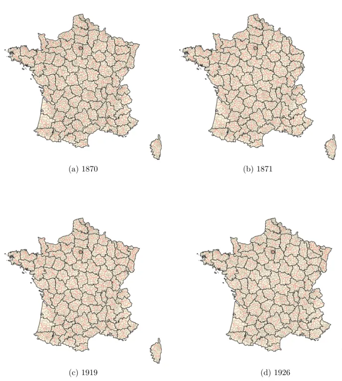
Overall, except for these two events and the creation of five dozen cantons, general ad-ministrative constituencies remained relatively stable throughout the Third Republic (Ozouf-Marignier and Verdier, 2009; 2013).16 Appendix Figure A.4 displays the evolution of their number between 1870 and 1940: from 87 to 90 départements, from 279 to 385 arrondisse-ments, and from 2,861 to 3,028 cantons. Figure 3 shows the geographic configuration of these administrative constituencies at four key dates: 1870, 1871, 1919, and 1926.
2.3.2. Special administrative constituencies
Military constituencies The territorial organization of the military prevalent during most of the Third Republic was based on a series of reforms passed in 1873–1874 (Boulanger, 2001, 15–37; Chanet, 2006). At its core, the law of “general organization of the army” of July 24, 1873, ensured consistency between military recruitment and military command. It divided the territory into 18 military regions, each further divided into eight subdivisions per the decree of August 6, 1874. Moreover, per the decree of September 28, 1873, one army corps per military region was created. Each army corps was composed of two infantry divisions of two brigades with two regiments—one infantry regiment per subdivision of military region. In each subdivision of military region was located a recruitment bureau, which managed recruitment and mobilization under the authority of the military region command. Although they overlapped geographically, military regions were the relevant administrative structures for recruitment, while army corps were relevant for military command.
Except for the regions of Paris and Lyon, which had specific military governments, delin-eations of military regions and subdivisions followed canton and arrondissement boundaries 14Changes that occurred under German rule between 1871 and 1918 are documented in Appendix Table A.3. 15Territorial changes induced by this reform are documented in Appendix Table A.4.
so as to maintain balance in terms of population, transportation networks, topography, and cultural homogeneity. This organization was not fundamentally altered until 1940, though it underwent a series of modifications. Until the early-1920s, the military adapted its territorial organization mostly along the north-eastern border in order to ensure efficient mobilization in case of military conflict with Germany.17 After its recovery in 1919, the military organi-zation in Alsace-Lorraine followed the same logic. Modifications from the late 1920s onward were instead dominated by the willingness of the military command of nesting subdivisions of military regions into département boundaries, which was nearly achieved by the mid-1930s. At odds with this system, the military organization that prevailed before the reforms of 1873–1874 did not exhibit such consistency between military recruitment and military command. It simply divided troops into six army corps across 22 divisions along départe-ment boundaries.18 Appendix Figure A.5 displays the evolution of the number of military constituencies between 1874 and 1940: from 18 to 20 military regions, and from 100 to 156 subdivisions of military regions.
The construction of annual constituency-level shapefiles for military corps and divisions (1870–1873) and military regions and subdivisions (1874–1940) is based on their characteri-zation in terms of general administrative constituencies. While they overlapped département boundaries between 1870 and 1873, military constituencies generally followed cantons and arrondissement boundaries between 1874 and 1940. For this period, I first match each can-ton from the TRF-GIS cancan-ton-level nomenclature 1874 to its military region and subdivision following the decree of August 6, 1874. Then, for each year onward, I update this initial configuration with territorial modifications to both cantons and military constituencies.19
Annual constituency-level shapefiles for military regions and subdivisions (1874–1940) exhibit the same limitations as canton-level shapefiles, as some subdivisions of military re-gions were defined across canton and commune boundaries.20 Following the same logic as for canton-level shapefiles, I create pseudo-military constituencies whenever relevant, mostly in the vicinity of the larger urban centers of Paris, Lyon, and Marseille. Appendix Figure A.6 displays the geographic configuration of military constituencies at four key dates: 1870, 1874, 1919, and 1940.
17Among the main modifications, a 20th military region (Nancy) was created in 1898 through the splitting of
the 6th military region (Châlons-sur-Marne) as well as a 21st military region (Épinal) by the end of 1913 through the splitting of the 7th military region (Besançon).
18The territorial configuration of military divisions in 1870 is documented in Appendix Table A.6. 19The 35 territorial modifications to military constituencies are documented in Appendix Table A.7.
20For instance, from 1874 onward, all but one subdivision of the 2nd military region (Amiens) were composed
of fractions of the cantons of Saint-Denis and Pantin (Seine), as well as fractions of the 10th, 19th, and 20th municipal arrondissements of Paris.
Judicial and penitentiary constituencies France’s judicial organization remained broadly stable from the early nineteenth century to the end of the Third Republic (Farcy, 1992, 29–47). Ordinary judicial institutions consisted of five nested jurisdictional levels. At the first level, justices of the peace (justices de paix) and simple police courts (tribunaux de
sim-ple police) had cantons as constituency and were headed by the same cantonal judge. Their
attributions were limited to minor civil cases that could be resolved by conciliation and to minor criminal offenses. The second level was constituted by courts of first instance
(tri-bunaux de première instance), the ordinary first-degree jurisdiction for civil cases, which also
ruled on appeals to justices of the peace. In criminal matters, its criminal courts (tribunaux
correctionnel) ruled on all offenses for which sentences were shorter than five years but
ex-ceeded those imposed by simple police courts. Until the decree of September 3, 1926, courts of first instance had arrondissements as constituency—except for the département of Seine, which had only one, and the arrondissement of Puget-Théniers, which had none. These courts were located at the subprefecture, barring a dozen exceptions. In the spirit of the arrondissements reform of 1926, the judicial reform of the same year suppressed 228 courts of first instance. However, this reform soon failed and all but six courts were reinstated in 1930 per the law of August 22, 1929—three courts were later suppressed in 1931–1932. At the third level, assize courts (cours d’assises) were autonomous départemental jurisdictions that ruled on crimes. They were only in session for one trimester each year except for the assize court of Paris, which was permanent. The fourth jurisdictional level was constituted by courts of appeal (cours d’appel), which ruled on appeals to courts of first instance, both in civil and criminal matters. There were 26–28 courts of appeal, each composed of one (Bastia) to seven (Paris) départements. Their delineations remained stable throughout the Third Republic barring modifications induced by the annexation and recovery of Alsace-Lorraine.21 Finally, the higher jurisdiction was the Court of Cassation (Cour de Cassation), which reviewed other courts’ rulings in last resort, both in civil and criminal matters. Panels a and b of Appendix Figure A.7 display the evolution of the number of judicial constituencies between 1870 and 1940: from 26 to 28 courts of appeal, and from 138 to 370 courts of first instance.
The construction of annual constituency-level shapefiles for courts of appeal is straight-forward as these followed département boundaries. For courts of first instance, I rely on their delineations along canton boundaries—although courts of first instance were based on ar-rondissements until 1929, their delineations from 1930 to 1940 were based on the geography of arrondissements prior to the reform of 1926, which left cantons untouched. I first match each canton from the TRF-GIS canton-level nomenclature 1870 to its court of first instance. 21The courts of appeal of Metz and Colmar were suppressed in 1871, the later being reinstated in 1919.
Then, for each year onward, I update this initial configuration with territorial modifications to both cantons and courts of first instance.22 Because justices of the peace, police courts, and assize courts had cantons and départements as constituencies, their geographies and nomenclatures follow that of these general administrative constituencies. Appendix Figure A.8 displays the geographic configuration of judicial constituencies at four key dates: 1870, 1871, 1926, and 1940.
Besides ordinary judicial institutions, special jurisdictions ruled over litigation specific to some professional groups, such as commercial courts (tribunaux de commerce) and labor courts (conseils de prud’hommes). Because these only existed in some cities and had het-erogeneous constituencies, I do not provide nomenclatures and shapefiles for these special jurisdictions. Annual commune nomenclatures do, however, detail their locations.
Finally, linked to the judicial system, the penitentiary system was administered through regional constituencies that comprised several départements from 1871 onward—in 1870, penitentiary constituencies and départements were confounded. Their number decreased over time, from 45 in 1871–1887 to 16 in 1926–1940 (Appendix Figure A.7, Panel c).23 Appendix Figure A.9 displays the geographic configuration of penitentiary constituencies at four key dates: 1871, 1888, 1909, and 1940.
Electoral constituencies The Third Republic was a Parliamentarian regime in which the National Assembly, France’s Lower House, elected the head of the executive branch (to-gether with the Senate from 1875 onward). Members of the National Assembly, the députés, were elected by male citizens aged 21 and older through a single-member system, with one député per electoral constituency, denominated circonscription—though the general elections of 1871, 1885, 1919, and 1924 used a block-list system. While block-list elections generally had département-level electoral constituencies, arrondissements formed the basis of electoral constituencies throughout the Third Republic (Gaudillère, 1995; Marty, 2013). Its electoral geography was based on the redistricting of 1875, which followed three principles that barely changed during the next seven decades: each arrondissement had at least one député, and therefore constituted at least one circonscription; each additional hundred thousand inhabi-tants entitled an arrondissement to an additional député; and a circonscription was modified only if its number of députés had to change due to population growth. There was only one major redistricting after 1875: that of 1927 after the return of the single-member system, which was broadly based on the geography of arrondissements prior to the reform of 1926.
22Modifications that affected courts of appeal and courts of first instance, along with other details, are
docu-mented in Appendix Table A.8.
The redistricting of 1889, also after the return to the single-member system, was essentially identical to that of 1875. Still, the population rule for redistricting entailed marginal changes after each census, adjusting constituencies in 10–20 arrondissement every five years.24 Panel a of Appendix Figure A.10 displays the evolution of the number of circonscriptions dur-ing the Third Republic: from 87 to 100 for block-list elections, and from 526 to 598 for single-member elections.
The construction of annual circonscription-level nomenclatures and shapefiles relies on two elements: TRF-GIS annual canton-level nomenclatures and Gaudillère’s (1995) Atlas
Historique des Circonscriptions Électorales Françaises, which provides maps of
circonscrip-tions from 1815 to 1986 for each département, with cantons as underlying frame. Using Gaudillère’s (1995) 800-page atlas, I manually match each contemporaneous canton to its electoral constituency for each redistricting year. I then expand these configurations to the following years until the next redistricting, taking into account territorial changes to cantons through TRF-GIS annual canton-level nomenclatures. I use the same methodology but at the level of communes (and of municipal arrondissements of Paris) for the départements of Seine and Seine-et-Oise as circonscriptions were generally defined at such levels in these two départements.
Annual circonscription-level shapefiles exhibit the same limitations as canton-level shape-files, as some circonscriptions were defined across canton and commune boundaries due to the population rule for redistricting. For instance, the city of Montluçon was divided along canton boundaries into the circonscriptions of Montluçon-1 (canton of Montluçon-Est) and Montluçon-2 (canton of Montluçon-Ouest) during single-member elections. Following the same logic as with canton-level shapefiles, I create pseudo-circonscriptions whenever rele-vant. Appendix Figure A.11 displays the geographic configuration of electoral constituencies at four key general elections dates: 1876, 1914, 1919, and 1928.
Academic constituencies The administration of public education during the Third Re-public was operated through a system of regional academies that was defined in 1854 and that overlapped département boundaries. Since then, each academy was administered by a rector who supervised primary, secondary, and higher education within the academy. He was assisted by several academic inspectors—one per département, two or more in the populous départements of Nord and Seine. The territorial configuration of the 17 academies that ex-isted by 1870 was seldom modified during the Third Republic.25 Panel b of Appendix Figure
24Appendix Table A.9 documents all 13 redistricting laws enacted during the Third Republic.
25In 1871, the Territoire-de-Belfort was transferred to the academy of Besançon; in 1888, the chef-lieu of the
academy of Douai was transferred to Lille; in 1919, the recovered département of Moselle was transferred to the academy of Strasbourg; and in 1920, the academy of Chambéry was suppressed and its départements
A.10 displays the evolution of the number of academies during the Third Republic, which remained at 16–17.
The construction of annual academy-level shapefiles is straightforward as academies were supra-départemental constituencies that underwent little modifications. I first match each département from the TRF-GIS département-level nomenclature 1870 to its academy per the decrees of August 22nd, 1854, and June 13th, 1860. Then, for each year onward, I update this initial configuration with territorial modifications to both départements and academies.26 Panel a of Appendix Figure A.12 displays the geographic configuration of academic constituencies in 1919.
Labor inspection constituencies The service of labor inspection of the Ministry of La-bor was created by the law of May 19th, 1874, which objective was to regulate child laLa-bor. However, it was not until the law of December 13th, 1892 that a service of labor inspectors structured the territory in order to control the application of labor regulations (Chetcuti and Le Noël, 1998). It was initially organized into 11 supra-départemental constituencies, each headed by one divisional inspector. Divisional inspectors were assisted by several départe-mental inspectors operating in territorial sections—92 in total. Labor inspection constituen-cies underwent little modifications after 1892.27 Panel c of Appendix Figure A.10 displays the evolution of the number of labor inspection constituencies during the Third Republic, which remained at 11–12.
To construct annual labor inspection-level shapefiles, I first match each canton from the TRF-GIS canton-level nomenclature 1892 to its labor inspection constituency per the law of December 13th, 1892—although these constituencies were supra-départemental, cantons of the département of Isère were initially split between the 10th and 11th constituency. Then, for each year onward, I update this initial configuration with territorial modifications to both cantons and labor inspection constituencies. Panel b of Appendix Figure A.12 displays the geographic configuration of labor inspection constituencies in 1919.
Ecclesiastical constituencies Despite the Separation of the Churches and the State in 1905, catholic ecclesiastical constituencies (dioceses) continued to play an important role
(Savoie and Haute-Savoie) transferred to the academy of Grenoble (Marichal, 1962, 751–9).
26The few territorial modifications to academies are documented in Appendix Table A.10.
27The sieges of the 2nd and 4th constituencies were respectively transferred from Châteauroux to Tours
and from Bar-le-Duc to Nancy in 1893; the département of Isère, initially split between the 10th and 11th constituency, was reunited into the 11th constituency in 1902; and the département of Somme was transferred from the 5th to the 6th constituency in 1911, then back to the 5th constituency in 1919. After World War I, a 12th constituency was created with Strasbourg as chef-lieu in order to structure labor inspections in the départements of Moselle, Bas-Rhin, and Haut-Rhin.
in the French society and to produce statistics (Sorrel, 2013). Inherited from the geog-raphy of Roman provinces, most dioceses were created between the second and the fifth centuries. Their delineations were substantially altered twice after the Revolution: by the Concordat of 1801, which broadly nested the diocesan geography into that of the newly created départements, and by the Papal bull Paternae charitatis of 1822, which restored some prerevolutionary dioceses (Duquesnoy, 2020). By 1870, the metropolitan territory was divided into 86 dioceses, among which 17 archbishoprics (archevêchés) and 69 bishoprics (évêchés). Ruled by an archbishop, archbishoprics were metropolitan sees and headed the territories of several subordinate bishoprics. Some episcopal sees were immediately subject to the Holy See—the dioceses of Metz and Strasbourg after 1919. Throughout the Third Republic, the territories of most dioceses followed département boundaries. Still, some fol-lowed arrondissements.28 The diocese of Carcassonne (Aude) even had an enclave in the département of Ariège through the canton of Quérigut. The diocesan geography of the dé-partements of Savoie and Haute-Savoie was more complex, as it divided their territories along commune boundaries (Deloche, 2017).29 Dioceses boundaries underwent little changes during the Third Republic.30 Panel d of Appendix Figure A.10 displays the evolution of the number of dioceses between 1870 and 1940, which remained at 84–87.
To construct annual diocese-level shapefiles, I first match each canton from the TRF-GIS canton-level nomenclature 1870 to its diocese per the Papal bull of 1822, taking into account the creation of the diocese of Laval in 1855. Then, for each year onward, I update this initial configuration with territorial modifications to both cantons and dioceses. I use the same methodology but at the level of communes for the départements of Savoie and Haute-Savoie. Panel c of Appendix Figure A.12 displays the geographic configuration of dioceses in 1919, together with the extent of metropolitan bishoprics.
3. Data Records
The TRF-GIS database is composed of two types of data files: annual constituency-level nomenclatures and annual constituency-constituency-level shapefiles.31 Annual constituency- and
28The diocese of Marseille, which corresponded to the arrondissement of Marseille; the diocese of Reims, which
corresponded to the département of Ardennes and the arrondissement of Reims (Marne); the diocese of Fréjus, which corresponded to the département of Var and the arrondissement of Grasse (Alpes-Maritimes) until 1886; the dioceses of Lille and Cambrai, which split the département of Nord after 1913.
29This configuration is documented in Appendix Table A.11.
30Beyond those described above, the Territoire-de-Belfort was transferred from the diocese of Strasbourg to
that of Besançon after the Franco-Prussian War, and the territories of the département of Meurthe-and-Moselle were attributed to the diocese of Nancy. Appendix Table A.12 documents these changes.
31A description of each these data files’ names, content, formats, sizes, and locations is available in Appendix
commune-level nomenclatures are available in Stata data format (.dta) as well as in text delimited format (.txt), with the main file-specific metadata replicated as notes within .dta files and along with separate codebooks for .txt files. Each annual constituency-level shapefile is composed of a (zipped) set of five files: a shape format file (.sph), a shape index format file (.shx), an attribute format file (.dbf), a projection description file (.prj), and a character encoding file (.cpg). These shapefiles use an RGF93 Lambert-93 projection, IGN’s reference projection system. I further follow IGN’s methodology and provide shapefiles both in polygon and vector forms. Shapefiles metadata are also provided for each constituency in QGIS metadata format (.qmd). Furthermore, separate datasets of chefs-lieux coordinates are provided in .csv format—these coordinates correspond to the current locations of their city halls.
The TRF-GIS follows FAIR data management practices (Wilkinson et al., 2016). Data files are available in the TRF-GIS Dataverse, hosted by the Harvard Dataverse, under the CC-BY 4.0 license at https://dataverse.harvard.edu/dataverse/TRF-GIS. Therein, each constituency constitutes a separate dataset—15 datasets in total. Each dataset is attributed a unique and persistent Digital Object Identifier (DOI) for better findability and citabil-ity. Data files are curated through DataCite Metadata Schema 4.3 and use the Library of Congress Subject Heading (LCSH) controlled vocabulary for topic classification.
3.1. General administrative constituencies
Départements Annual département-level nomenclatures are composed of 10 variables (Appendix Table A.24). They include départements’ codes, names, and whether they were composed of enclaved territories and islands (e.g., the Enclave des Papes of the département of Vaucluse, enclaved in the territory of the département of Drôme). They also include information on départements’ chefs-lieux (prefectures): their INSEE codes, names, whether they are current or former communes (e.g., the prefecture of the département of Ardennes was located in the former commune of Mézières), and their geographic coordinates. For départements codification, I give number 99 to the département of Meurthe in 1870. Cod-ifications and toponyms are otherwise standard. Note that although the TRF-GIS treats the Territoire-de-Belfort as a département, it did not achieve this status officially until 1922. Annual département-level shapefiles contain the same variables as département-level nomen-clatures.
Appendix Table A.22 for judicial and penitentiary constituencies, and in Appendix Table A.23 for electoral, academic, labor inspection, and ecclesiastical constituencies. Appendix Table A.23 also describes data files of commune-level nomenclatures.
Arrondissements Annual arrondissement-level nomenclatures are composed of 15 vari-ables (Appendix Table A.24). They include arrondissements’ département code and name as well as arrondissements’ codes and names. They also include information on arrondisse-ments’ chefs-lieux (subprefectures): their INSEE codes, names, whether they are current or former communes, whether they were common to other arrondissements (e.g., Strasbourg was the subprefecture of the arrondissements of Strasbourg-Campagne and of Strasbourg-Ville), whether they were located outside of their arrondissement (e.g., Strasbourg was located outside of the arrondissement of Strasbourg-Campagne), and their geographic coordinates. Arrondissements one-digit codification uniquely identifies arrondissements within départe-ments and follows the COG 2011. For arrondissedéparte-ments that no longer existed by then, I assign a higher number in ascending alphabetical order within each département and keep this codification constant so that arrondissements can be uniquely identified across time. Moreover, I keep the contemporaneous toponymy of arrondissements, which names gener-ally were that of their subprefectures.32 Note that although the TRF-GIS treats municipal arrondissements of Paris and the Territoire-de-Belfort as arrondissements, these territories did not have this status officially. Annual arrondissement-level shapefiles contain the same variables as arrondissement-level nomenclatures.
Cantons Annual canton-level nomenclatures are composed of 18 variables (Appendix Ta-ble A.24). They include cantons’ département and arrondissement codes and names as well as cantons’ codes, names, and communal composition. The later variable, which follows INSEE’s COGs codification convention, indicates whether a canton was composed of entire communes and/or of fractions of communes (e.g., the canton of Montluçon-Est was com-posed of eight entire communes and a fraction of the commune of Montluçon). They also include information on cantons’ chefs-lieux (bureaux centralisateurs): their INSEE codes, names, whether they are current or former communes, whether they were common to other cantons (e.g., Montluçon was the bureau centralisateur of both cantons of Montluçon-Est and Montluçon-Ouest), and their geographic coordinates. Cantons two-digit codification uniquely identifies cantons within départements and follows the COG 2011. For cantons that no longer existed by then, I use the codification in the COG 1954. For those that no longer existed by 1954, I assign a higher number in ascending alphabetical order within each département and keep this codification constant so that cantons can be uniquely identified across time. Moreover, I keep the contemporaneous toponymy of cantons, which names
gen-32Appendix Table A.13 documents the ten toponymic modifications to arrondissements that occurred during
erally included that of their bureau centralisateur.33 Note that although the TRF-GIS treats municipal arrondissements of Paris as cantons, these territories did not have this status of-ficially. Moreover, the communes of partially annexed cantons that had remained in France after the Franco-Prussian War were not re-assigned to functioning cantons until 1873. As a result, their chefs-lieux were (virtually) outside of France in 1871 and 1872.34
Because the commune-level GEOFLA 2011 shapefile forms the base frame for annual canton-level shapefiles, and cantons were sometimes defined across commune boundaries, TRF-GIS shapefiles do not entirely match canton-level nomenclatures. Instead, they use the concept of canton. Following INSEE’s and IGN’s codification conventions, pseudo-cantons are assigned codes greater than 80 in ascending alphabetical order within départe-ments. Moreover, their toponymy corresponds to the common city infra-communal cantons are aggregated into. For instance, in the case of the Montluçon area displayed in Figure 2, canton-level shapefiles contain the pseudo-canton of Montluçon, which extent corresponds to the commune of Montluçon and which is given pseudo-canton code 80. During the Third Re-public, 10–12 percent of cantons were composed of fractions of communes, which translated into 110–120 pseudo-cantons (Figure A.4, Panel c).35 Annual canton-level shapefiles contain the same variables as canton-level nomenclatures, except that their base units are pseudo-cantons rather than pseudo-cantons. To reflect this difference, variables prefix in these shapefiles is pct rather than ct.
3.2. Special administrative constituencies
Military constituencies (1870–1873) Annual military corps-level nomenclatures are composed of 10 variables (Appendix Table A.25). They include military corps’ codes, names, and composition (entire départements). They also include information on military corps’ chefs-lieux: their INSEE codes, names, whether they are current or former communes, and their geographic coordinates. Codifications and toponyms are contemporaneous, with to-ponyms corresponding to military corps chefs-lieux. Annual military corps-level contain the same variables as military corps-level nomenclatures.
Annual military division-level nomenclatures are composed of 14 variables (Appendix Table A.25). They include military divisions’ corps code and name as well as military divi-sions’ codes, names, and composition (entire départements). They also include information 33Appendix Table A.14 documents the 206 toponymic modifications to cantons that occurred during the Third
Republic.
34This was the case for 36 communes of the annexed cantons of Gorze (Moselle), Vic-sur-Seille and Lorquin
(Meurthe), and Saales and Schirmeck (Vosges).
35Appendix Table A.15 documents the mapping between cantons and pseudo-cantons—this mapping is also
on military divisions’ chefs-lieux: their INSEE codes, names, whether they are current or for-mer communes, and their geographic coordinates. Codifications and toponyms are contem-poraneous, with toponyms corresponding to military divisions chefs-lieux. Annual military divisions-level shapefiles contain the same variables as military divisions-level nomenclatures.
Military constituencies (1874–1940) Annual military region-level nomenclatures are composed of 10 variables (Appendix Table A.25). They include military regions’ codes, names, and composition. For instance, throughout the Third Republic, the 2nd military re-gion (Amiens) was composed of fractions of arrondissements and of entire cantons. They also include information on military regions’ chefs-lieux: their INSEE codes, names, whether they are current or former communes, and their geographic coordinates. Codifications and to-ponyms are contemporaneous, with toto-ponyms corresponding to military regions chefs-lieux. Because the commune-level GEOFLA 2011 shapefile forms the base frame for military region-level shapefiles, and military regions were sometimes defined across cantons and commune boundaries, these shapefiles do not entirely correspond to military region-level nomencla-tures. Instead, these shapefiles use the concept of pseudo-military region. Pseudo-military regions are assigned military region codes greater than 90 in ascending alphabetical order, and their names correspond to their territorial composition. For instance, the city of Lyon was divided between the military regions of Grenoble and Besançon from 1874 to 1921. This pseudo-military region is assigned pseudo-region code 90 and name “Grenoble - Be-sançon.” Pseudo-military regions are not assigned a chef-lieu, so all variables with prefix cl are empty for actual pseudo-military regions.36 Annual military region-level shapefiles con-tain the same variables as military region-level nomenclatures, except that their base units are pseudo-military regions rather than military regions. To reflect this difference, variables prefix in these shapefiles is pmreg rather than mreg. In addition, the variable pmreg_type indicates whether military regions were effectively pseudo-military regions.
Annual military subdivision-level nomenclatures are composed of 15 variables (Appendix Table A.25). They include military subdivisions’ region code and name as well as military subdivisions’ codes, names, and composition. They also include information on military subdivisions’ chefs-lieux: their INSEE codes, names, whether they are current or former communes, whether they were common to other subdivisions (e.g., Rouen was the chef-lieu of both military subdivisions of Rouen-Nord and Rouen-Sud), and their geographic coordinates. Codifications and toponyms are contemporaneous, with toponyms corresponding to military subdivisions chefs-lieux. Because the commune-level GEOFLA 2011 shapefile forms the base 36Appendix Table A.16 documents the mapping between pseudo-cantons and pseudo-military regions. This
frame for military subdivision-level shapefiles, and military subdivisions were sometimes defined across cantons and commune boundaries, these shapefiles do not entirely correspond to military subdivision-level nomenclatures. Instead, these shapefiles use the concept of pseudo-military subdivision. Pseudo-military subdivisions are assigned military subdivision codes greater than 10 in ascending alphabetical order, and their names correspond to their territorial composition. For instance, the city of Rouen was divided between the military subdivisions of Rouen-Nord and Rouen-Sud from 1874 to 1929. This pseudo-military region is assigned code 11 and name “Rouen (Nord - Sud).” Pseudo-military subdivisions are not assigned a chef-lieu, so all variables with prefix cl are empty for actual pseudo-military subdivisions.37 Annual military subdivision-level shapefiles contain the same variables as military subdivision-level nomenclatures, except that their base units are pseudo-military subdivisions rather than military subdivisions. To reflect this difference, variables prefix in these shapefiles is pmsub rather than msub. In addition, the variable pmsub_type indicates whether military subdivisions were effectively pseudo-military subdivisions.38
Judicial and penitentiary constituencies Annual court of appeal-level nomenclatures are composed of 9 variables (Appendix Table A.26). They include courts of appeal’s codes and names, as well as information on their chefs-lieux: their INSEE codes, names, and geographic coordinates. Toponyms are contemporaneous and correspond to courts of appeal chefs-lieux. Courts of appeal two-digit codification uniquely identifies these constituencies over time and is assigned in ascending alphabetical order. Annual court of appeal-level shapefiles contain the same variables as court of appeal-level nomenclatures.
Annual court of first instance-level nomenclatures are composed of 14 variables (Appendix Table A.26). They include their court of appeal’s code and name, as well as courts of first instances’ codes and names. They also include information on courts of first instances’ chefs-lieux: their INSEE codes, names, whether they were also a subprefecture, and their geographic coordinates. Toponyms are contemporaneous and correspond to courts of first instance chefs-lieux. Courts of first instance two-digit codification uniquely identifies these constituencies over time within their court of appeal and is assigned in ascending alphabetical order. Annual court of first instance-level shapefiles contain the same variables as court of first instance-level nomenclatures.
Annual penitentiary constituency-level nomenclatures are composed of 9 variables (Ap-pendix Table A.26). They include penitentiary constituencies’ codes and names, as well as 37Appendix Table A.17 documents the mapping between pseudo-cantons and pseudo-military subdivisions.
This mapping is also available as a dataset alongside annual military subdivision-level nomenclatures.
38Appendix Table A.18 documents the composition of pseudo-military subdivisions in terms of military
information on their chefs-lieux: their INSEE codes, names, and geographic coordinates. Toponyms are contemporaneous and correspond to penitentiary constituencies’ chefs-lieux. Penitentiary constituencies two-digit codification uniquely identifies these constituencies over time and is based on the contemporaneous codification defined in the official act of 1871 re-organizing penitentiary constituencies—for 1870, these correspond to département codes; penitentiary constituencies created after 1871 are assigned codes that are ascending in the temporal order of their creation. Annual penitentiary constituency-level shapefiles contain the same variables as penitentiary constituency-level nomenclatures.
Electoral constituencies Annual circonscription-level nomenclatures are composed of 6 variables (Appendix Table A.27). They include circonscriptions’ département code as well as circonscriptions’ codes, names, and composition. The later variable indicates whether a cir-conscription was composed of entire départements, arrondissements, cantons, or communes. Some codes specifically refer to the circonscriptions of Paris. Contrary to other constituen-cies, electoral constituencies are uniquely identified by their name, which corresponds to their arrondissement name, with the addition of a number for the larger urban centers, or, between 1928 and 1940, to the most important city of the constituency—sometimes two ad-joined names, such as “Nantua - Gex.” For convenience, I provide a codification in ascending alphabetical order within each département, but it is not necessarily consistent over time due to the changing nature of circonscriptions’ boundaries. Likewise, urban circonscriptions which contemporaneous names were composed of the arrondissement name and a number, such as “Saint-Denis-3” in Seine-et-Oise, might not be consistent over time—this is gener-ally the case in the more urban areas in which redistricting was frequent. Moreover, no chefs-lieux are indicated as electoral circonscriptions were not administrative units, but only territorial constituencies—electoral operations were instead coordinated at cantons’ bureaux centralisateurs. Each annual circonscription-level nomenclature further indicates three el-ements among its metadata: the election system (block-list or single-member), whether it was a general election year, and the relevant redistricting year. Annual circonscription-level shapefiles contain the same variables as circonscription-level nomenclatures, except that their base units are pseudo-circonscriptions rather than circonscriptions. To reflect this difference, variables prefix in these shapefiles is pcirco rather than circo. In addition, the variable pcirco_type indicates whether circonscriptions were effectively pseudo-circonscriptions.39
39Because shapefiles are stored in associated .dbf files, attributes names cannot be longer than 10
charac-ters. Consequently, two field names are abbreviated: pcirco_name into pcirco_nam and pcirco_type into pcirco_typ.
Academic constituencies Annual academy-level nomenclatures are composed of 8 vari-ables (Appendix Table A.27). They include academies’ codes and names, as well as infor-mation on their chefs-lieux: their INSEE codes, names, and geographic coordinates. To-ponyms are contemporaneous and correspond to academies chefs-lieux. Academies two-digit codification uniquely identifies these constituencies over time and is assigned in ascending alphabetical order—except for the academy of Chambéry, created in 1860 and suppressed in 1919, which holds academy code 17. Annual academy-level shapefiles contain the same variables as academy-level nomenclatures.
Labor inspection constituencies (1892–1940) Annual labor inspection-level nomen-clatures are composed of 6 variables (Appendix Table A.27). They include labor inspections codes, as well as information on their chefs-lieux: their INSEE codes, names, and geographic coordinates. Labor inspection constituencies did not have a specific toponymy beyond their 2-digit codification, which was fixed over time. Annual labor inspection-level shapefiles con-tain the same variables as labor inspection-level nomenclatures.
Ecclesiastical constituencies Annual diocese-level nomenclatures are composed of 14 variables (Appendix Table A.27). They include the archbishopric’s code and name each diocese was attached to, its type (metropolitan see or exempt), as well as dioceses codes, names, and types (archbishoprics or bishoprics). They further include information on their chefs-lieux: their INSEE codes, names, and geographic coordinates. The diocesan toponymy is contemporaneous and corresponds to customary dioceses names, which consisted in the locations of their chefs-lieux (episcopal sees)—except for the diocese of Aire, which episcopal see was transferred to Dax in 1933, and for the diocese of Tarentaise, which name referred the Tarentaise Valley. Different from their customary names, dioceses’ formal names were com-posed of all prerevolutionary dioceses their bishops were entitled. For instance, by 1854, the bishop of Bayeux was entitled the former diocese of Lisieux. As a result, the formal name of the diocese of Bayeux became “Bayeux-Lisieux.” These names were sometimes cumbersome: for instance, by 1877, the formal name of the diocese of Avignon was “Avignon-Apt-Cavaillon-Carpentras-Orange-Vaison.” Annual diocese-level nomenclatures therefore use dioceses cus-tomary names.40 Dioceses two-digit codification uniquely identifies these constituencies over time and are assigned in ascending alphabetical order—except for the archbishopric of the dioceses of Metz and Strasbourg after 1919, exempt and subject to the Holy See, which is assigned code 99. Annual diocese-level shapefiles contain the same variables as diocese-level nomenclatures.
3.3. Annual commune-level nomenclatures
Annual commune-level nomenclatures are composed of 69 variables (Appendix Table A.28). Each commune can be identified through its unique Cassini code from the HAC database as well as through its INSEE code in 2005 geography.41 Communes toponyms are contemporaneous. These nomenclatures include the names and codes of all the above general and special administrative constituencies each commune belonged to in a given year—pseudo-constituencies in the cases of cantons, military regions and subdivisions, and electoral cir-conscriptions. They also include indicator variables for whether a commune was the chef-lieu of a constituency or the siege of a special jurisdiction: a commercial or a labor court (Farcy, 1992, 875–86). Appendix Table A.28 describes the 21 additional variables included in annual commune-level nomenclatures that are not present in other constituency-level nomenclatures.
To enable users to combine statistics produced by administrations at different and po-tentially ex-ante incompatible levels of aggregation, commune-level nomenclatures further provide population counts from the HAC database, which reports this information based on population censuses.42 The During the Third Republic, population censuses were carried out every five years—except in 1871, when it was postponed to 1872 due to the Franco-Prussian War, and in 1916, when it was canceled due to the First World War. Three variables relate to population counts: pop, the census population count, ipop, the interpolated population count, and pop_flag, a population count flag. The pop variable is missing outside of census years (extended missing value .a) and for a few communes during census years: when a com-mune was created during the same year as a census but after it was carried out (.b), when the census archive was lost (.c) or unreadable (.d), and when the commune was not enumer-ated (.e). Except in 1872, when 233 communes were not enumerenumer-ated (nearly exclusively in the département of Hautes-Pyrénées) and the archives for another 482 communes were lost (exclusively in the département of Vosges), missing population counts during census years remain negligible: they always account for less than 15 communes—less than 3 communes in 9 out of all 13 censuses that were carried out during the Third Republic. Based on these raw population counts, the variable ipop provides interpolated population counts for all years and all communes present in annual commune-level nomenclatures. The variable pop_flag
41Communes that disappeared between 1943 and 2005 hold the INSEE code assigned by the first official
nomenclature, the COG of 1943. Those that disappeared before 1943 hold the INSEE code of their absorbing commune. The variable com_act differentiates between these cases.
42These population counts correspond to the total population (population totale), which includes the municipal
population (population municipale) and the population in collective dwellings (population comptée à part). Population counts for municipal arrondissements of Paris are from the Dénombrements de la Population volumes, which are available onepsilon.insee.fr(accessed May 2021).
documents which imputation method is used: none for census years (1), linear interpolation for inter-census years (2), linear interpolation for census years when the census archive was lost (3) or unreadable (4), linear interpolation for census years when a commune was not surveyed (5), and imputation from the previous (6) or next (7) census for communes that were created or suppressed during an inter-census year. Imputations remain limited to about 30 communes across all years after 1872, and to about a hundred in 1870–1871.
Finally, annual commune-level nomenclatures have a specific treatment of Paris: they pro-vide both municipal arrondissement and commune-level information. Municipal arrondisse-ments of Paris hold INSEE codes 75101–75120, and the commune of Paris, INSEE code 75056. Whenever Paris is the chef-lieu of a constituency, this prerogative falls onto the first municipal arrondissement as well as onto the commune. Whenever it is subdivided into con-stituencies, the commune of Paris holds the status of pseudo-constituency with corresponding codifications: it holds pseudo-canton code 7580, pseudo-military region and subdivision code 99, and pseudo-circonscription code 99.
4. Technical Validation
4.1. TRF-GIS nomenclatures
Information supporting TRF-GIS nomenclatures documented in secondary sources were thoroughly verified against primary sources.43 Appendix Table A.29 details the content of each of the 175 primary sources used for this verification procedure: the constituency they are relevant to, their codification (date of official issue and type), their title, their persistent identifier (PID) assigned by Gallica and the National Library of France (BNF) in archival resource key (ARK) form, and their origin. Primary sources’ types take the following forms: law (L), decree (D), order (A, for arrêté), ordinance (O), and papal bull (B). Their origins is generally the Journal Officiel, though sometimes it is the Bulletin des Lois, the Code
Pénitentaire or Code des Prisons, the Bulletin Administratif de l’Instruction Publique, and
the Acta Apostolicae Sedis. All these primary sources are available in PDF format in the TRF-GIS dataverse. This rigorous verification procedure combined with data integrity tests in the TRF-GIS source code enabled to identify 231 inaccuracies or errors in the HAC database and to rectify them.44
43These secondary sources include the HAC database (Motte, Séguy and Théré, 2003; Motte and Vouloir, 2007)
as well as Marichal (1962), Masson (1984), Farcy (1992), Gaudillère (1995), Chetcuti and Le Noël (1998), Boulanger (2001), Chanet (2006), Marignier and Verdier (2009), Verdier (2009), Marty (2013), Ozouf-Marignier and Verdier (2013), Deloche (2017), and Duquesnoy (2020).
Nomenclatures were also verified against periodical statistical publications of relevant ad-ministrations, among which censuses for general administrative constituencies, the Compte
Rendu sur le Recrutement de l’Armée for military constituencies, the Compte Général de l’Administration de la Justice Civile et Commerciale and the Compte Général de l’Administration de la Justice Criminelle for judicial constituencies, the Statistique Pénitentiaire for
peniten-tiary constituencies, and the Tableau des Élections à la Chambre des Députés for electoral constituencies.45
4.2. TRF-GIS shapefiles
IGN’s GEOFLA 2011 shapefile constitutes the underlying frame of TRF-GIS shapefiles. As discussed above, I use this dataset for quality and reproducibility purposes: it constitutes the official representation of France’s communes in 2011 geography and is available under open licensing. Although IGN’s BD CARTO® shapefiles are far more precise than the GE-OFLA (1:25,000 against 1:1,000,000), these files are not all freely accessible. Their use would therefore substantially alter the possibilities of reproduction and dissemination of TRF-GIS shapefiles. Moreover, their manipulation is more cumbersome: while GEOFLA is available as an ensemble, BD CARTO files are only available separately for each département, and their overall size approaches 2.5 GB against 150 MB for the GEOFLA. In the end, the lower precision of the GEOFLA need not be very problematic because TRF-GIS shapefiles aim at regional and national extents (see Section 2.2).
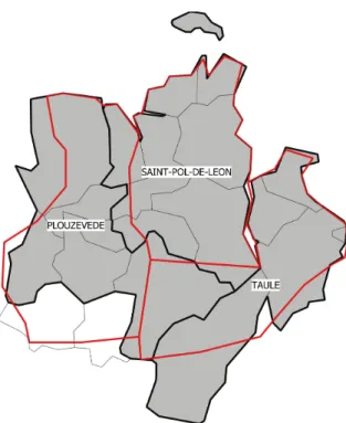
The general methodology used to construct TRF-GIS shapefiles offers several advantages over the manual vectorization of georeferenced historical maps (as in, e.g., LARHRA, 2011; Perret, Gribaudi and Barthelemy, 2015; Ostafin et al., 2020). First, it yields more precise results than existing outputs, such as LARHRA’s (2011) cantons shapefiles for 1884 and 1925: historical maps with national extents oftentimes lacked precision and had unspecified projection systems, making the resulting georeferencing potentially approximate, and ur-ban centers, Corsica, and islands challenging to vectorize.46 Typical inaccuracies that result from these methods are displayed in Figure 4, which plots three randomly selected cantons from TRF-GIS and LARHRA cantons shapefiles 1884. Five out of twenty communes (which territories did not change historically) are classified in the wrong canton by LARHRA’s (2011) shapefile.47 Second, and more importantly, historical maps are generally not
avail-45Useful to interested users, an up-to-date listing of the availability of these periodical statistical publications
is available athttps://progedo.hypotheses.org/514(accessed May 2021).
46For instance, historical cantons maps of 1884 and 1925 have a precision of 1:1,250,000 and 1:1,600,000,
respectively.
47More precisely, misclassified communes are Plougar (Plouvézédé instead of Plouescat), Plougourvest