Cutting the Electric Bill for Internet-Scale Systems

Cutting the Electric Bill for Internet-Scale Systems

The MIT Faculty has made this article openly available.

Please share

how this access benefits you. Your story matters.

Citation

Qureshi, Asfandyar et al. “Cutting the electric bill for internet-scale

systems.” Proceedings of the ACM SIGCOMM 2009 conference on

Data communication. Barcelona, Spain: ACM, 2009. 123-134. Print.

As Published

http://doi.acm.org/10.1145/1592568.1592584

Publisher

Association for Computing Machinery

Version

Author's final manuscript

Citable link

http://hdl.handle.net/1721.1/50995

Terms of Use

Attribution-Noncommercial-Share Alike 3.0 Unported

Cutting the Electric Bill for Internet-Scale Systems

Asfandyar Qureshi

Rick Weber

Hari Balakrishnan

John Guttag

Bruce Maggs

Carnegie Mellon University bmm@cs.cmu.edu

ABSTRACT

Energy expenses are becoming an increasingly important fraction of data center operating costs. At the same time, the energy expense per unit of computation can vary sig-nificantly between two different locations. In this paper, we characterize the variation due to fluctuating electricity prices and argue that existing distributed systems should be able to exploit this variation for significant economic gains. Electricity prices exhibit both temporal and geographic vari-ation, due to regional demand differences, transmission inef-ficiencies, and generation diversity. Starting with historical electricity prices, for twenty nine locations in the US, and network traffic data collected on Akamai’s CDN, we use sim-ulation to quantify the possible economic gains for a realistic workload. Our results imply that existing systems may be able to save millions of dollars a year in electricity costs, by being cognizant of locational computation cost differences.

Categories and Subject Descriptors

C.2.4 [Computer-Communication Networks]: Distributed Systems

General Terms

Economics, Management, Performance

1.

INTRODUCTION

With the rise of “Internet-scale” systems and “cloud com-puting” services, there is an increasing trend toward massive, geographically distributed systems. The largest of these are made up of hundreds of thousands of servers and several data centers. A large data center may require many megawatts of electricity [1], enough to power thousands of homes.

Millions of dollars must be spent annually on the electric-ity needed to power one such system. Furthermore, these already large systems are increasing in size at a rapid clip, outpacing data center energy efficiency gains [2], and elec-tricity prices are expected to rise.

Permission to make digital or hard copies of all or part of this work for personal or classroom use is granted without fee provided that copies are not made or distributed for profit or commercial advantage and that copies bear this notice and the full citation on the first page. To copy otherwise, to republish, to post on servers or to redistribute to lists, requires prior specific permission and/or a fee.

SIGCOMM’09,August 17–21, 2009, Barcelona, Spain. Copyright 2009 ACM 978-1-60558-594-9/09/08 ...$10.00.

Company Servers Electricity Cost

eBay 16K ∼0.6×105_{MWh ∼$3.7M} Akamai 40K ∼1.7×105_{MWh ∼$10M} Rackspace 50K ∼2×105_{MWh ∼$12M} Microsoft >200K >6×105_{MWh >$36M} Google >500K >6.3×105MWh >$38M USA (2006) 10.9M 610×105_{MWh $4.5B} MIT campus 2.7×105_{MWh $62M}

Figure 1: Estimated annual electricity costs for large companies (servers and infrastructure) @ $60/MWh. These are conservative estimates, meant to be lower bounds. See §2.1 for derivation details. For scale, we have included the actual 2007 consumption and utility bill for the MIT campus, including dormitories and labs. Organizations such as Google, Microsoft, Amazon, Ya-hoo!, and many other operators of large networked systems cannot ignore their energy costs. A back-of-the-envelope cal-culation for Google suggests it consumes more than $38M worth of electricity annually (figure 1). A modest 3% reduc-tion would therefore exceed a million dollars every year. We project that even a smaller system like Akamai’s1 _consumes

an estimated $10M worth of electricity annually2.

The conventional approach to reducing energy costs has been to reduce the amount of energy consumed [3, 4]. New cooling technologies, architectural redesigns, DC power, multi-core servers, virtualization, and energy-aware load balanc-ing algorithms have all been proposed as ways to reduce the power demands of data centers. That work is complemen-tary to ours.

This paper develops and analyzes a new method to reduce the energy costs of running large Internet-scale systems. It relies on two key observations:

1. Electricity prices vary. In those parts of the U.S. with wholesale electricity markets, prices vary on an hourly basis and are often not well correlated at different lo-cations. Moreover, these variations are substantial, as much as a factor of 10 from one hour to the next. If, when computational demand is below peak, we can dy-namically move demand (i.e., route service requests) to places with lower prices, we can reduce energy costs. 2. Large distributed systems already incorporate request

routing and replication. We observe that most Internet-scale systems today are geographically distributed, with

1

This paper covers work done outside Akamai and does not rep-resent the official views of the company.

2

Though Akamai seldom pays directly for electricity, it pays for it indirectly as part of co-location expenses.

machines at tens or even hundreds of sites around the world. To provide clients good performance and to tolerate faults, these systems implement some form of dynamic request routing to map clients to servers, and often have mechanisms to replicate the data necessary to process requests at multiple sites.

We hypothesize that by exploiting these observations, large systems can save a significant amount of money, using mech-anisms for request routing and replication that they already implement. To explore this hypothesis, we develop a simple cost-aware request routing policy that preferentially maps requests to locations where energy is cheaper.

Our main contribution is to identify the relevance of elec-tricity price differentials to large distributed systems and to estimate the cost savings that could result in practice if the scheme were deployed.

Problem Specification. Given a large system composed of server clusters spread out geographically, we wish to map client requests to clusters such that the total electricity cost (in dollars, not Joules) of the system is minimized. For sim-plicity, we assume that the system is fully replicated. Addi-tionally, we optimize for cost every hour, with no knowledge of the future. This rate of change is slow enough to be com-patible with existing routing mechanisms, but fast enough to respond to electricity market fluctuations. Finally, we in-corporate bandwidth and performance goals as constraints. Existing frameworks already exist to optimize for bandwidth and performance; modeling them as constraints makes it possible to add our process to the end of the existing opti-mization pipeline.

Note that our analysis is concerned with reducing cost, not energy. Our approach may route client requests to distant locations to take advantage of cheap energy. These longer paths may cause overall energy consumption to rise slightly. Energy Elasticity. The maximum reduction in cost our approach can achieve hinges on the energy elasticity of the clusters. This is the degree to which the energy consumed by a cluster depends on the load placed on it. Ideally, clusters would draw no power in the absence of load. In the worst case, there would be no difference between the peak power and the idle power of a cluster. Present state-of-the-art sys-tems [5, 6] fall somewhere in the middle, with idle power being around 60% of peak. A system with inelastic clusters is forced to always consume energy everywhere, even in re-gions with high energy prices. Without adequate elasticity, we cannot effectively route the system’s power demand away from high priced areas.

Zero-idle power could be achieved by aggressively consol-idating, turning off under-utilized components, and always activating only the minimum number of machines needed to handle the offered load. At present, achieving this without impacting performance is still an open challenge. However, there is an increasing interest in energy-proportional servers [6] and dynamic server provisioning techniques are being ex-plored by both academics and industry [7, 8, 9, 10, 11].

Results. To conduct our analysis, we use trace-driven simulation with real-world hourly (and daily) energy prices obtained from a number of data sources. We look at 39 months of hourly electricity prices from 29 US locations. Our request traces come from the Akamai content distribu-tion network (CDN): we obtained 24-days worth of request

traffic data (five-minute load) for each server cluster located at a commercial data center in the U.S. We used these data sets to estimate the performance of our simple cost-aware routing scheme under different constraints.

We show that:

• Existing systems can reduce energy costs by at least 2%, without any increase in bandwidth costs or sig-nificant reduction in client performance (assuming a Google-like energy elasticity, an Akamai-like server dis-tribution and 95/5 bandwidth constraints). For large companies this can exceed a million dollars a year. • Savings rapidly increase with energy elasticity: in a

fully elastic system, with relaxed bandwidth constraints, we can reduce energy cost by over 30% (around 13% if we impose strict bandwidth constraints), without a significant increase in client-server distances.

• Allowing client-server distances to increase leads to in-creased savings. If we remove the distance constraint, a dynamic solution has the potential to beat a static solution (i.e., place all servers in cheapest market) by a substantial margin (45% maximum savings versus 35% maximum savings).

Presently, energy cost-aware routing is relevant only to very large companies. However, as we move forward and the energy elasticity of systems increases, not only will this routing technique become more relevant to the largest sys-tems, but much smaller systems will also be able to achieve meaningful savings.

Paper Organization. In the next section, we provide some background on server electricity expenditure and sketch the structure of US energy markets. In section 3 we present data about the variation in regional electric prices. Section 4 describes the Akamai data set used in this paper. Section 5 outlines the energy consumption model used in the simu-lations covered in section 6. Section 7 considers alternative mechanisms for market participation. Section 8 presents some ideas for future work, before we conclude.

2.

BACKGROUND

This section first presents evidence that electricity is be-coming an increasingly important economic consideration, and then describes the salient features of the wholesale elec-tricity markets in the U.S.

2.1

The Scale of Electricity Expenditures

In absolute terms, servers consume a substantial amount of electricity. In 2006, servers and data centers accounted for an estimated 61 million MWh, 1.5% of US electricity con-sumption, costing about 4.5 billion dollars [3]. At worst, by 2011, data center energy use could double. At best, by re-placing everything with state-of-the-art equipment, we may be able to reduce usage in 2011 to half the current level [3]. Most companies operating Internet-scale systems are se-cretive about their server deployments and power consump-tion. Figure 1 shows our estimates for several such com-panies, based on back-of-the-envelope calculations3_{. The}

3_{Energy in Wh ≈ n·(P}

idle+(Ppeak−Pidle)·U +(P U E−1)·Ppeak)·

365 · 24, where: n is server count, Ppeakis server peak power in

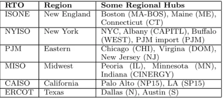
RTO Region Some Regional Hubs

ISONE New England Boston (MA-BOS), Maine (ME),

Connecticut (CT)

NYISO New York NYC, Albany (CAPITL), Buffalo

(WEST), PJM import (PJM)

PJM Eastern Chicago (CHI), Virgina (DOM),

New Jersey (NJ)

MISO Midwest Peoria (IL), Minnesota (MN),

Indiana (CINERGY)

CAISO California Palo Alto (NP15), LA (SP15)

ERCOT Texas Dallas (N), Austin (S)

Figure 2: The different regions studied in this paper. The listed hubs provide a sense of RTO coverage and a reference to map electricity market location identifiers (hub NP15) to real locations (Palo Alto).

server numbers are from public disclosures for eBay [12] and Rackspace (Q1 2009 earnings report). To calculate energy, we have made the following assumptions: average data cen-ter power usage effectiveness (PUE)4 _{is 2.0 [3] and is}

cal-culated based on peak power; average server utilization is around 30% [6, 7]; average peak server power usage is 250 Watts (based on measurements of actual servers at Akamai); and idle servers draw 60-75% of their peak power [5, 8]. Our numbers for Microsoft are based on company statements [13] and energy figures mentioned in a promotional video [14].

To estimate Google’s power consumption, we assumed 500K servers (based on an old, widely circulated number [13]), operating at 140 Watts each [5], a PUE of 1.3 [4] and average utilization around 30% [6]. Such a system would consume more than 6.3 × 105MWh, and would incur an an-nual electricity bill of nearly $38 million (at $60 per MWh wholesale rate). These numbers are consistent with an in-dependent calculation we can make. comScore estimated that Google performed about 1.2B searches/day in August 2007 [15], and Google officially stated recently that each search takes 1 kJ of energy on average (presumably amor-tized to include indexing and other costs). Thus, search alone works out to 1 × 105 _{MWh in 2007. Google’s servers}

handle GMail, YouTube, and many other applications, so our earlier estimates seem reasonable. Google may well have more than a million servers [1], so an annual electric bill ex-ceeding $80M wouldn’t be surprising.

Akamai’s electricity costs represent indirect costs not seen by the company itself. Like others who rely on co-location facilities, Akamai seldom pays directly for electricity. Power is mostly built into the billing model, with charges based on provisioned capacity rather than consumption. In section 7 we discuss why our ideas are relevant even to those not directly charged per-unit of electricity they use.

2.2

Wholesale Electricity Markets

Although market details differ regionally, this section pro-vides a high-level view of deregulated electricity markets, providing a context for the rest of the paper. The discus-sion is based on markets in the United States.

Generation. Electricity is produced by government util-ities and independent power producers from a variety of sources. In the United States, coal dominates (nearly 50%), followed by natural gas (∼20%), nuclear power (∼20%), and hydroelectric generation (6%) [16].

4_{A measure of data center energy efficiency.}

Different regions may have very different power genera-tion profiles. For example, in 2007, hydroelectric sources accounted for 74% of the power generated in Washington state, while in Texas, 86% of the energy was generated us-ing natural gas and coal.

Transmission. Producers and consumers are connected to an electric grid, a complex network of transmission and distribution lines. Electricity cannot be stored easily, so supply and demand must continuously be balanced.

In addition to connecting nearby nodes, the grid can be used to transfer electricity between distant locations. The United States is divided into eight reliability regions, with varying degrees of inter-connectivity. Congestion on the grid, transmission line losses (est. 6% [17] in 2006), and boundaries between regions introduce distribution inefficien-cies and limit how electricity can flow.

Market Structure. In each region, a pseudo-government-al body, a Regionpseudo-government-al Transmission Organization (RTO), man-ages the grid (figure 2). An RTO provides a central author-ity that sets up and directs the flow of electricauthor-ity between generators and consumers over the grid. RTOs also provide mechanisms to ensure the short-term reliability of the grid. Additionally, RTOs administer wholesale electricty mar-kets. While bilateral contracts account for the majority of the electricity that flows over the grid, wholesale electric-ity trading has been growing rapidly, and presently covers about 40% of total electricity.

Wholesale market participants can trade forward contracts for the delivery of electricity at some specified hour. In or-der to determine prices for these contracts, RTOs such as PJM use an auctioning mechanism: power producers present supply offers (possibly price sensitive), consumers present demand bids (possibly price sensitive); and a coordinating body determines how electricity should flow and sets prices. The market clearing process sets hourly prices for the dif-ferent locations in the market. The outcomes depend not only on bids and offers, but also account for a number of constraints (grid-connectivity, reliability, etc.).

Each RTO operates multiple parallel wholesale markets. There are two common market types:

Day-ahead markets (futures) provide hourly prices for delivery during the following day. The outcome is based on expected load5_.

Real-time markets (spot) are balancing markets where prices are calculated every five minutes or so, based on actual conditions, rather than expectations. Typically, this market accounts for a small fraction of total energy transactions (less than 10% of total in NYISO). Generally speaking, the most expensive active generation resource determines the market clearing price for each hour. The RTO attempts to meet expected demand by activating the set of resources with the lowest operating costs. When demand is low, the base-load power plants, such as coal and nuclear can fulfill it. When demand rises, additional re-sources, such as natural gas turbines, need to be activated. Security constraints, line losses and congestion costs also impact price. When transmission system restrictions, such as line capacities, prevent the least expensive energy sup-plier from serving demand, congestion is said to exist. More

$/MWh Portland, OR (MID-C) 50 100 150 $/MWh Richmond, VA (Dominion) 50 100 150 $/MWh Houston, TX (ERCOT-H) 50 100 150 $/MWh Palo Alto, CA (NP15) 0 50 100 150

Jan 06 May 06 Sep 06 Jan 07 May 07 Sep 07 Jan 08 May 08 Sep 08 Jan 09 May

Figure 3: Daily averages of day-ahead peak prices at different hubs [18]. The elevation in 2008 correlates with record

high natural gas prices, and does not affect the hydroelectric dominated Northwest. The Northwest consistently

experiences dips near April (this seems to be correlated with seasonal rainfall). Correlated with the global economic downturn, recent prices in all four locations exhibit a downward trend.

0 25 50 75 100 125 2009-02-10 2009-02-14 2009-02-18 Price $/MWh

Mon Tue Wed Thu Fri Sat Sun Mon Tue Wed Real-time 5-min Real-time hourly Day-ahead hourly

0 25 50 75 100 125 2009-03-03 2009-03-07 2009-03-11 Price $/MWh Time (EST/EDT)

Mon Tue Wed Thu Fri Sat Sun Mon Tue Wed

Figure 4: Comparing price variation in different whole-sale markets, for the New York City hub. The top graph shows a period when prices were similar across all mar-kets; the bottom graph shows a period when there was significantly more volatility in the real-time market. expensive generation units will then need to be activated, driving up prices. Some markets include an explicit conges-tion cost component in their prices.

Surprisingly, negative prices can show up for brief periods, representing conditions where if energy were to be consumed at a specific location at a specific time the overall efficiency of the system would increase.

Market boundaries introduce economic transaction ineffi-ciencies. As we shall see later, even geographically close lo-cations in different markets tend to see uncorrelated prices. Part of the problem is that different markets have evolved using different rules, pricing models, etc.

Clearly, the market for electricity is complex. In addition to the factors mentioned here, many local idiosyncrasies ex-ist. In this paper, we use a relatively simple market model that assumes the following:

1. Real-time prices are known and vary hourly.

2. The electric bill paid by the service operator is propor-tional to consumption and indexed to wholesale prices. 3. The request routing behavior induced by our method does not significantly alter prices and market behavior. The validity of the second assumption depends upon the extent to which companies hedge their energy costs by con-tractually locking in fixed pricing (see section 7). A large

Window 5 min 1 hr 3 hr 12 hr 24 hr

Real-time σ 28.5 24.8 21.9 18.1 15.6

Day-ahead σ N/A 20.0 19.4 17.1 16.0

Figure 5: The real-time market is more variable at short time-scales than the day-ahead market. Standard devi-ations for Q1 2009 prices at the NYC hub are shown, averaged using different window sizes.

body of economic literature deals with the structure and evo-lution of energy markets [19, 20, 21], market failures, and arbitrage opportunities for securities traders (e.g. [22, 23]).

3.

EMPIRICAL MARKET ANALYSIS

We posit that imperfectly correlated variations in local electricity prices can be exploited by operators of large geo-graphically distributed systems to save money. Rather than presenting a theoretical discussion, we take an empirical ap-proach, grounding our analysis in historical market data ag-gregated from government sources [19, 16], trade publication archives [18], and public data archives maintained by the dif-ferent RTOs. We use price data for 30 locations, covering January 2006 through March 2009.

3.1

Price Variation

Geographic price differentials are what really matter to us, but it is useful to first get a feel for the behaviour of individual prices.

Daily Variation. Figure 3 shows daily average prices for four locations6, from January 2006 through April 2009. Although prices are relatively stable at long time scales, they exhibit a significant amount of day-to-day volatility, short-term spikes, seasonal trends, and dependencies on fuel prices and consumer demand. Some locations in the figure are visibly correlated, but hourly prices are not correlated (§3.2). Different Market Types. Spot and futures markets have different price dynamics. Figures 4 and 5 illustrate the difference for NYC. Compared to the day-ahead market, the hourly real-time (RT) market is more volatile, with more high-frequency variation, and a lower average price. The underlying five minute RT prices are even more volatile.

6_{The Northwest is an important region, but lacks an hourly}

wholesale market, forcing us to omit the region from the remain-der of our analysis.

Location RTO Mean∗ _StDev∗ _Kurt.∗

Chicago, IL PJM 40.6 26.9 4.6

Indianapolis, IN MISO 44.0 28.3 5.8

Palo Alto, CA CAISO 54.0 34.2 11.9

Richmond, VA PJM 57.8 39.2 6.6

Boston, MA ISONE 66.5 25.8 5.7

New York, NY NYISO 77.9 40.26 7.9

Figure 6: Real-time market statistics, covering

hourly prices from January 2006 through March 2009

(∗_{statistics are from the 1% trimmed data).}

0 0.05 0.10 0.15 0.20 0.25 -40 -20 0 20 40 Hourly price change $/MWh

78% samples 89% µ=0.0 σ=37.2 κ=17.8 -40 -20 0 20 40 Hourly price change $/MWh

82% 96%

µ=0.0 σ=22.5 κ=33.3

(a) Palo Alto (NP15) (b) Chicago (PJM)

Figure 7: Histograms of hour-to-hour change in real-time hourly prices for two locations, over the 39-month period. Both distributions are zero-mean, Gaussian-like, with very long tails.

For the remainder of this paper, we focus exclusively on the RT market. Our goal is to exploit geographically uncor-related volatility, something that is more common in the RT market. We restrict ourselves to hourly prices, but speculate that the additional volatility in five minute prices provides further opportunities.

Figure 6 provides additional statistics for hourly RT prices. Hour-to-Hour Volatility. As seen in figure 4, the hour-to-hour variation in NYC’s RT prices can be dramatic. Fig-ure 7 shows the distribution of the hourly change for Palo Alto and Chicago. At each location, the price per MWh changed hourly by $20 or more roughly 20% of the time. A $20 step represents 50% of the mean price for Chicago. Fur-thermore, the minimum and maximum price during a single day can easily differ by a factor of 2.

The existence of rapid price fluctuations reflects the fact that short term demand for electricity is far more elastic than supply. Electricity cannot always be efficiently moved from low demand areas to high demand areas, and producers cannot always ramp up or down easily.

3.2

Geographic Correlation

Our approach would fail if hourly prices are well correlated at different locations. However, we find that locations in different regional markets are never highly correlated, even when nearby, and that locations in the same region are not always well correlated.

Figure 8 shows a scatter-plot of pairwise correlation and geographic distance7_{. No pairs were negatively correlated.}

Note how correlation decreases with distance. Further, note the impact of RTO market boundaries: most pairs drawn from the same RTO lie above the 0.6 correlation line, while all pairs from different regions lie below it8. We also see

7_{We have verified our results using subsets of the data (e.g. last}

12 months), mutual information (Ix,y), shifted signals, etc.

8_I

x,ymuch more clearly divides the data between same-RTO and

different-RTO pairs, suggesting that the small overlap in figure 8 is due to the existence of non-linear relationships within NYISO

0 0.2 0.4 0.6 0.8 1 1 10 100 1000 Correlation coefficient

Est. distance between two hubs (km) Different RTOs NYISO ISONE PJM MISO ERCOT CAISO

Figure 8: The relationship between price correlation, distance, and parent RTO. Each point represents a pair of hubs (29 hubs, 406 pairs), and the correlation coef-ficient of their 2006-2009 hourly prices (> 28k samples each). Red points represent paired hubs from different RTOs; blue points are labelled with the RTO of both.

-100 -50 0 50 100

Difference $/MWh Sat Sun Mon Tue Wed Thu Fri Sat Sun Mon Tue Wed Thu Fri Sat PaloAlto minus Richmond Austin minus Richmond

-100 -50 0 50 100 2008-08-11 2008-08-18 Difference $/MWh Time (EDT)

Sat Sun Mon Tue Wed Thu Fri Sat Sun Mon Tue Wed Thu Fri Sat

Figure 9: Variation of price differentials with time. a surprising lack of diversity within some regions: LA and Palo Alto have a coefficient of 0.94.

Hourly prices are not correlated at short time-scales, but we should not expect prices to be independent. Natural gas prices, for example, will introduce some coupling (see figure 3) between distant locations.

3.3

Price Differentials

Figure 9 shows hourly price differentials for two pairs of locations over an eight day period (both pairs have mean differentials close to zero). The three locations are far from each other and in different RTOs. We see price spikes (some extend far off the scale, the largest is $1900) and extended periods of price asymmetry. Sometimes the asymmetry favours one, sometimes the other. This suggests that a pre-determined assignment of clients to servers is not optimal.

Differential Distributions. Consider two locations. In order for our dynamic approach to yield substantial savings over a static solution, the price differential between those locations must vary in time, and the distribution of this dif-ferential should ideally have a zero mean and a reasonably high variance. Such a distribution would imply that neither site is strictly better than the other, but also that a dynamic solution, always buying from whichever site is least expen-sive that hour, could yield meaningful savings. Additionally, the dynamic approach could win when presented with two locations having uncorrelated periods of price elevation. and ERCOT, not detected by the correlation coefficient.

0 0.1 -100 -50 0 50 100 price difference $/MWh µ=0.0 σ=55.7 κ=10 0 0.1 -100 -50 0 50 100 price difference $/MWh µ=0.9 σ=87.7 κ=466 0 0.1 -100 -50 0 50 100 price difference $/MWh µ=-12.3 σ=52.5 κ=146 0 0.1 0.2 0.3 0.4 -100 -50 0 50 100 price difference $/MWh µ=-17.2 σ=31.3 κ=20 0 0.1 -100 -50 0 50 100 price difference $/MWh µ=-4.2 σ=32.0 κ=32

(a) PaloAlto - Virginia (b) Austin - Virginia (c) Boston - NYC (d) Chicago - Virginia (e) Chicago - Peoria

Figure 10: Price differential histograms for five location pairs and 39 months of hourly prices.

-50 0 50

Jan 06 May 06 Sep 06 Jan 07 May 07 Sep 07 Jan 08 May 08 Sep 08 Jan 09

(PaloAlto - Richmond) $/MWh

Figure 11: PaloAlto-Virginia price differential distribu-tions for each month. The monthly median prices and inter-quartile range are shown.

Figure 10 shows the pairwise differential distributions for some locations, for the 2006-2009 data. The California-Virginia (figure 10a) and Texas-California-Virginia (figure 10b) dis-tributions are zero-mean with a high variance. There are many other such pairs9_.

Boston-NYC (figure 10c) is skewed, since Boston tends to be cheaper than NYC, but NYC is less expensive 36% of the time (the savings are greater than $10/MWh 18% of the time). Thus, even with such a skewed distribution, there exists an opportunity to dynamically exploit differentials for meaningful savings.

Unsurprisingly, a number of pairs exist where one location is strictly better than the other, and dynamic adaptation is unnecessary. Chicago-Virginia (figure 10d) is an example: Virginia is less expensive 8% of the time, but the savings almost never exceed $10/MWh.

The dispersion introduced by a market boundary can be seen in the dynamically exploitable Chicago-Peoria distribu-tion (figure 10e).

Evolution in Time. The price differential distributions do not remain static in time. Figure 11 shows how the PaloAlto-Virginia distribution changed from month to month. A sustained price asymmetry may exist for many months, before reversing itself. The spread of prices in one month may double the next month.

Time-of-Day Price differentials depend on the time-of-day. For instance, because California and Virginia are in different time zones, peak demand does not overlap. This is likely an important factor shaping the price differential.

Figure 12 shows how the hour of day affects the differ-entials for three location pairs. For PaloAlto-Virginia, we see a strong dependency on the hour. Before 5am (eastern), Virginia has a significant edge; by 6am the situation has re-versed; from 1-4pm neither is better. For Boston-NYC we see a different kind of dependency: from 1am-7am neither

9

There are 60 other pairs (a set of 16 hubs) with |µ| ≤ 5 ∧ σ ≥ 50; and 86 pairs (a set of 28 hubs) with |µ| ≤ 5 ∧ σ ≥ 25.

-25 0 25 50

$/MWh

PaloAlto minus Richmond

-25 0 25 50

$/MWh

Boston minus NYC

-25 0 25 50 0 3 6 9 12 15 18 21 $/MWh

Hour of day (EST/EDT) Chicago minus Peoria

Figure 12: Price differential distributions (median and inter-quartile range) for each hour of the day.

0.00 0.05 0.10

0 3 6 9 12 15 18 21 24 27 30 33 36

Fraction of total time

California-Virginia differential duration (hours)

Figure 13: For PaloAlto-Virginia, short-lived price dif-ferentials account for most of the time.

site is better, at all other times Boston has the edge. The effect of hour-of-day on Chicago-Peoria is less clear.

Differential Duration. We define the duration of a sus-tained price differential as the number of hours one location is favoured over another by more than $5/MWh. As soon as the differential falls below this threshold, or reverses to favour the other location, we mark the end of the differential. Figure 13 shows how much time was spent in short-duration price-differentials, for PaloAlto-Virginia. Short differentials (<3 hrs) are more frequent than other types. Medium length differentials (<9 hrs) are common. Differentials that last longer than a day are rare, for a balanced pair like this.

4.

AKAMAI: TRAFFIC AND BANDWIDTH

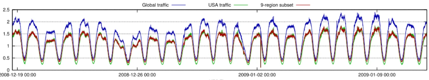
In order to understand the interaction of real workloads with electricity prices, we acquired a data set detailing traffic on Akamai’s infrastructure. The data covers 24 days worth of traffic on a large subset of Akamai’s servers, with a peak of over 2 million hits/sec (figure 14). The 9-region traffic is the subset of servers for which we have electricity price data. We use the Akamai traffic because it is a realistic work-load. Akamai has over 2000 content provider customers in the US. Hence, the traffic represents a broad user base.

0 0.5 1 1.5 2 2.5 2008-12-19 00:00 2008-12-26 00:00 2009-01-02 00:00 2009-01-09 00:00 Million hits/sec UTC Time

Global traffic USA traffic 9-region subset

Figure 14: Traffic in the Akamai data set. We see a peak hit rate of over 2 million hits per second. Of this, about 1.25 million hits come from the US. The traffic in this data set comes from roughly half of the servers Akamai runs. In comparison, in total, Akamai sees around 275 billion hits/day.

However, Akamai does not use aggressive server power management, their CDN is sensitive to latency and their workload contains a large fraction of computationally triv-ial hits (e.g., fetches of well cached objects). So our work is far less relevant to Akamai than to systems where more energy elasticity exists and workloads are computationally intensive. Furthermore, in mapping clients to servers, Aka-mai’s system balances a number of concerns—trying to opti-mize performance, handle partially replicated CDN objects, optimize network bandwidth costs, etc.

Traffic Data. Traffic data was collected at 5-minute in-tervals on servers housed in Akamai’s public clusters. Aka-mai has two types of clusters: public, and private. Pri-vate clusters are typically located inside of universities, large companies, small ISPs, and ISPs outside the US. These clus-ters are dedicated to serving a specific user base, e.g., the members of a university community, and no others. Pub-lic clusters are generally located in commercial co-location centers and can serve any users world-wide. For any user not served by a private cluster, Akamai has the freedom to choose which of its public clusters to direct the user. Clients that end up at public clusters tend to see longer network paths than clients that can be served at private clusters.

The 5-minute data contains, for each public cluster: the number of hits and bytes served to clients; a rough geogra-phy of where those clients originated; and the load in each of the clusters. In addition, we surveyed the hardware used in the different clusters and collected values for observed server power usage. We also looked at the top-level mapping sys-tem to see how name-servers were mapped to clusters.

In the data we collected, the geographic localization of clients is coarse: they are mapped to states in the US, or countries. If multiple clusters exist in a city, we aggregate them together and treat them as a single cluster. This affects our calculation of client-server distances in §6.

Bandwidth Costs. An important contributor to data center costs is bandwidth, and there may be large differ-ences between costs on different networks, and sometimes on the same network over time. Bandwidth costs are signif-icant for Akamai, and thus their system is aggressively op-timized to reduce bandwidth costs. We note that changing Akamai’s current assignments of clients to clusters to reduce energy costs could increase its bandwidth costs (since they have been optimized already). Right now the portion of co-location cost attributable to energy is less than but still a significant fraction of the cost of bandwidth. The relative cost of energy versus bandwidth has been rising. This is primarily due to decreases in bandwidth costs.

We cannot cannot ignore bandwidth costs in our analysis. The complication is that the bandwidth pricing specifics are considered to be proprietary information. Therefore, our treatment of bandwidth costs in this paper will be relatively abstract.

Akamai does not view bandwidth prices as being geo-graphically differentiated. In some instances, a company as large as Akamai can negotiate contracts with carriers on a nationwide basis. Smaller regional providers may provide transit for free. Prices are usually set per network port, us-ing the basic 95/5 billus-ing model: traffic is divided into five minute intervals and the 95th percentile is used for billing.

Our approach in this paper is to estimate 95th percentiles from the traffic data, and then to constrain our energy-price rerouting so that it does not increase the 95th percentile bandwidth for any location.

Client-Server Distances. Lacking any network level data on clients, we use geographic distance as a coarse proxy for network performance in our simulations. We see some evidence of geo-locality in the Akamai traffic data, but there are many cases where clients are not mapped to the near-est cluster geographically. One reason is that geographical distance does not always correspond to optimal network per-formance. Another possibility is that the system is trying to keep those clients on the same network, even if Akamai’s servers on that network are geographically far away. Yet another possibility is that clients are being moved to distant clusters because of 95/5 bandwidth constraints.

5.

MODELING ENERGY CONSUMPTION

In order to estimate by how much we can reduce energy costs, we must first model the system’s energy consumption for each cluster. We use data from the Akamai CDN as a representative real-world workload. This data is used to de-rive a distribution of client activity, cluster sizes, and cluster locations. We then use an energy model to map prices and cluster-traffic allocations to electricity expenses. The model is admittedly simplistic. Our goal is not to provide accurate figures, but rather to estimate bounds on savings.

5.1

Cluster Energy Consumption

We model the energy consumption of a cluster as be-ing proportional, roughly linear, to its utilization. Multiple studies have shown that CPU utilization is a good estimator for power usage [5, 8]. Our model is adapted from Google’s empirical study of a data center [5] in which their model was found to accurately (less than 1% error) predict the dy-namic power drawn by a group of machines (20-60 racks).

We augment this model to fill in some missing pieces and parametrize it using other published studies and measure-ments of servers at Akamai.

Let Pcluster be the power usage of a cluster, and let utbe

its average CPU utilization (between 0 and 1) at time t: Pcluster(ut) = F (n) + V (ut, n) + ǫ

Where n is the number of servers in the cluster, F is the fixed power, V is the variable power, and ǫ is an empirically derived correction constant (see [5]).

F(n) = n ·`Pidle+ (P U E − 1) · Ppeak

´

V(ut, n) = n ·(Ppeak− Pidle) · (2ut− urt)

Where Pidleis the average idle power draw of a single server,

Ppeak is the average peak power, and the exponent r is an

empirically derived constant equal to 1.4 (see [5]). The equa-tion for V is taken directly from the original paper. A linear model (r = 1) was also found to be reasonably accurate [5]. We added the PUE component, since the Google study did not account for cooling etc.

With power-management, the idle power consumption of a server can be as low as 50-65% of the peak power consump-tion, which can range from 100-250W [5, 7, 8]. Without power-management an off-the-shelf server purchased in the last several years averages around 250W and draws ∼95% of its peak power when idle (based on measured values).

Ultimately, we want to use this model in simulation to estimate the maximum percentage reduction in the energy costs of some server deployment pattern. Consequently, the absolute values chosen for Ppeak and Pidleare unimportant:

their ratio is what matters. In fact, it turns out that the value Pcluster(0)

Pcluster(1) is critical in determining the savings that

can be achieved using price-differential aware routing. Ideally, Pcluster(0) would be zero: an idle cluster would

consume no energy. At present, achieving this without im-pacting performance is still an open challenge. However, there is an increasing interest in energy-proportional com-puting [6] and dynamic server provisioning techniques are being explored by both academics and industry [7, 8, 9, 10, 11]. We are confident that Pcluster(0) will continue to fall.

5.2

Increase in Routing Energy

In our scheme, clients may be routed to distant servers in search of cheap energy. From an energy perspective, this network path expansion represents additional work that must be performed by something. If this increase in energy were significant, network providers might attempt to pass the additional cost on to the server operators. Given what we know about bandwidth pricing (§4), a small increase in routing energy should not impact bandwidth prices. Alter-natively, server operators may bear all the increased energy costs (suppose they run the intermediate routers).

A simple analysis suggests that the increased path lengths will not significantly alter energy consumption. Routers are not designed to be energy proportional and the energy used by a packet to transit a router is many orders of magnitude below the energy expended at the endpoints (e.g., Google’s 1 kJ/query [24]). We estimate that the average energy needed for a packet to pass through a core router is on the order of 2 mJ [25]10_{. Further we estimate that the incremental} en-10

Reported for a Cisco GSR 12008 router: 540k mid-sized pack-ets/sec and 770 Watts measured.

ergy dissipated by each packet passing through a core router would be as low as a 50 µJ per medium-sized packet [25]11_.

We must also consider what happens if the new routes overload existing routers. If we use enough additional band-width through a router it may have to be upgraded to higher capacity hardware, increasing the energy significantly. How-ever, we could prevent this by incorporating constraints, like the 95/5 bandwidth constraints we use.

6.

SIMULATION: PROJECTING SAVINGS

In order to test the central thesis of this paper, we con-ducted a number of simulations, quantifying and analysing the impact of different routing policies on energy costs and client-server distance.

Our results show that electricity costs can plausibly be re-duced by up to 40% and that the degree of savings primarily depends on the energy elasticity of the system, in addition to bandwidth and performance constraints. We simulate Akamai’s 95/5 bandwidth constraints and show that overall system costs can be reduced. We also sketch the relation-ship between client-server distance and savings. Finally we investigate how delaying the system’s reaction to price dif-ferentials affects savings.

6.1

Simulation Strategy

We constructed a simple discrete time simulator that step-ped through the Akamai usage statistics, letting a routing module (with a global view of the network) allocate traffic to clusters at each time step. Using these allocations, we mod-eled each cluster’s energy consumption, and used observed hourly market prices to calculate energy expenditures. Be-fore presenting the results, we provide some details about our simulation setup.

Electricity Prices. We used hourly real-time market prices for twenty-nine different locations (hubs). However, we only have traffic data for Akamai public clusters in nine of these locations. Therefore, most of the simulations focused on these nine locations. Our data set contained 39 months of price data, spanning January 2006 through March 2009. Unless noted otherwise, we assumed the system reacted to the previous hour’s prices.

Traffic and Server Data. The Akamai workload data set contains 5-minute samples for the hits-per-second ob-served at public clusters in twenty five cities, for a period of 24 days and some hours. Each sample also provides a map, specifying where hits originated, grouping clients by state, and which city they were routed to.

We had to discard seven of these cities because of a lack of electricity market data for them. The remaining eighteen cities were grouped by electricity market hub, as nine ‘clus-ters’. In our 24-day simulation, we used the traffic incident on these nine clusters.

In order to simulate longer periods we derived a syn-thetic workload from the 24-day Akamai workload (US traf-fic only). We calculated an average hit rate For every hub and client state pair. We produced a different average for each hour of the day and each day of the week.

Additionally, the Akamai data allowed us to derive

capac-11_{Reported: power consumption of idle router is 97% the peak}

power. In the future, power-aware hardware may reduce this disparity between the marginal and average energy.

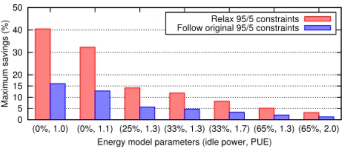
0 5 10 15 20 30 40 50 (0%, 1.0) (0%, 1.1) (25%, 1.3) (33%, 1.3) (33%, 1.7) (65%, 1.3) (65%, 2.0) Maximum savings (%)

Energy model parameters (idle power, PUE) Relax 95/5 constraints Follow original 95/5 constraints

Figure 15: The system’s energy elasticity is key in de-termining the degree of savings price-conscious routing can achieve. Further, obeying existing 95/5 bandwidth constraints reduces, but does not eliminate savings. The graph shows 24-day savings for a number of different

PUE and Pidlevalues with a 1500km distance threshold.

The savings for each energy model are given as a per-centage of the total electricity cost of running Akamai’s actual routing scheme under that energy model. ity constraints and the 95th percentile hits and bandwidth for each cluster. Capacity estimates were derived using ob-served hit rates and corresponding region load level data provided by Akamai. Our simulations use hits rather than the bandwidth numbers from the data.

Most of our simulations used Akamai’s geographic server distribution. Although the details of the distribution may introduce artifacts into our results, this is a real-world distri-bution. As such, we feel relying on it rather than relying on synthetic distributions makes our results more compelling.

Routing Schemes. In our simulations we look at two routing schemes: Akamai’s original allocation; and a dis-tance constrained electricity price optimizer.

Given a client, the price-conscious optimizer maps it to a cluster with the lowest price, only considering clusters within some maximum radial geographic distance. For clients that do not have any clusters within that maximum distance, the routing scheme finds the closest cluster and considers any other nearby clusters (< 50km). If the selected cluster is nearing its capacity (or the 95/5 boundary), the optimizer iteratively finds another good cluster.

The price optimizer has two parameters that modulate its behaviour: a distance threshold and a price threshold. Any price differentials smaller than the price threshold are ignored (we use $5/MWh). Setting the distance threshold to zero, gives an optimal distance scheme (select the cluster geographically closest to client); setting it to a value larger than the East-West coast distance gives an optimal price scheme (always select the cluster with the lowest price).

We are not proposing this as a candidate for implemen-tation, but it allows us to benchmark how well a price-conscious scheme could do and to investigate trade-offs be-tween distance constraints and achievable savings.

Energy Model. We use the cluster energy model from section 5.1. We simulated the running cost of the system using a number of different values for the peak server power (Ppeak), idle server power (Pidle) and the PUE. This section

discusses normalized costs and Pidleis always expressed as a

percentage of Ppeak. Some energy parameters that we used:

optimistic future (0% idle, 1.1 PUE); cutting-edge/google (60% idle, 1.3 PUE); state-of-the-art (65% idle, 1.7 PUE); disabled power management (95% idle, 2.0 PUE).

Client-Server Distance. Given a client’s origin state and the server’s location (hub), our distance metric calcu-lates a population-density weighted geographic distance. We used census data to derive basic population density functions for each US state. When the traffic contains clients from outside the US, we ignore them in the distance calculations. We use this function as a coarse measure for network dis-tance. The granularity of the Akamai data set does not pro-vide enough information for us to estimate network latency between clients and servers, or even to accurately calculate geographic distances between clients and servers.

6.2

At the Turn of the Year: 24 Days of Traffic

We begin by asking the question: what would have hap-pened if an Akamai-like system had used price conscious routing at the end of 2008? How would this have com-pared in cost and client-server distance to the current rout-ing methods employed by Akamai?

Energy Elasticity. We find that the answer hinges on the energy elasticity characteristics of the system. Figure 15 illustrates this. When consumption is completely propor-tional to load, using price-conscious routing could eliminate 40% of the electricity expenditure of Akamai’s traffic alloca-tion, without appreciably increasing client-server distances. As idle server power and PUE rise, we see a dramatic drop in possible savings: at Google’s published elasticity level (65% idle, 1.3 PUE), the maximum savings have dropped to 5%. Inelasticity constrains our ability to route power demand away from high prices.

Bandwidth Costs. A reduced electric bill may be over-shadowed by increased bandwidth costs. Figure 15 therefore also shows the savings when we prevent clusters from hav-ing higher 95th percentile hit rates than were observed in the Akamai data. We see that constraining bandwidth in this way may cause energy savings to drop down to about a third of their earlier values. However, the good news is that these savings are reductions in the total operating cost.

By jointly optimizing bandwidth and electricity, it should be possible to acquire part of the economic value represented by the difference between savings with and without band-width constraints.

Distance and Savings. The savings in figure 15 do not represent a free lunch: the mean client-server distance may need to increase to leverage market diversity.

The price conscious routing scheme we use has a dis-tance threshold parameter, allowing us to explore how higher client-server distances lead to lower electric bills. Figure 16 shows how increasing the distance threshold can be used to reduce electricity costs. Figure 17 shows how client-server distances change in response to changes in the threshold.

At a distance threshold of 1100km, the 99th percentile estimated client-server distances is at most 800km. This should provide an acceptable level of performance (the dis-tance between Boston and Alexandria in Virginia is about 650km and network RTTs are around 20ms).

At this threshold, using the future energy model, the sav-ings is significant, between 10% (obey 95/5 constraints) and 20%. There is an elbow at a threshold of 1500km, causing both savings and distances to jump (the distance between Boston and Chicago is about 1400km). After this, increas-ing the threshold provides diminishincreas-ing returns.

0.65 0.70 0.75 0.80 0.85 0.90 0.95 1.00 0 500 1000 1500 2000 2500

Normalized 24-day cost

Distance threshold (km) Akamai allocation

Follow original 95/5 constraints Relax 95/5 constraints

Figure 16: 24-day electricity costs fall as the distance threshold is increased. The costs shown here are for a (0% idle, 1.1 PUE) model, normalized to the cost of the Akamai allocation. 400 600 800 1000 1200 1400 1600 0 500 1000 1500 2000 2500 Client-Server distance (km) Distance threshold (km) Boston-DC Boston-Chicago mean distance (ignore 95/5) 99th percent (ignore 95/5) mean distance 99th percent

Figure 17: Increasing the distance threshold allows the routing of clients to cheaper clusters further away (figure 16 shows corresponding falling cost)

Figure 16 shows results for a specific set of server energy parameters, but other parameters give scaled curves with the same basic shapes (this follows analytically from our energy model equations in §5.1; the difference in scale can be seen in figure 15).

6.3

Synthetic Workload: 39 Months of Prices

The previous section uses a very small subset of the price data we have. Using a synthetic workload, derived from the original 24-day one, we ran simulations covering January 2006 through March 2009. Our results show that savings increase above those for the 24-day period.

Figure 18 shows how electricity cost varied with the dis-tance threshold (analogous to figure 16). The results are similar to what we saw for the 24-day case, but maximum savings are higher. Notably: thresholds above 2000km in figure 18 do not exhibit sharply diminishing returns like those seen in 16. In order to normalize prices, we used statis-tics of how Akamai routed clients to model an Akamai-like router, and calculated its 39-month cost.

Figure 19 breaks down the savings by cluster, showing the change in cost for each cluster. The largest savings is shown at NYC. This is not surprising since the highest peak prices tend to be in NYC. These savings are not achieved by always routing requests away from NYC: the likelihood of requests being routed to NYC depends on the time of day.

We simulated other server distributions (evenly distributed across all 29 hubs, heterogeneous distributions, etc) and saw similar decreasing cost/distance curves.

0.50 0.60 0.70 0.80 0.90 1.00 0 500 1000 1500 2000 2500 Normalized cost Distance threshold (km) Akamai-like routing

Only use cheapest hub Follow original 95/5 constraints Relax 95/5 constraints

Figure 18: 39-month electricity costs fall as the distance threshold is increased. The costs shown here are for a (0% idle, 1.1 PUE) model, normalized to the cost of the synthetic Akamai-like allocation.

-12% 10% -8% -6% -4% -2% 0 2% 4% CA1CA2 MA NY IL VA NJ TX1TX2 <500km -12% 10% -8% -6% -4% -2% 0 2% 4% CA1CA2 MA NY IL VA NJ TX1TX2 <1000km -12% 10% -8% -6% -4% -2% 0 2% 4% CA1CA2 MA NY IL VA NJ TX1TX2 <1500km -12% 10% -8% -6% -4% -2% 0 2% 4% CA1CA2 MA NY IL VA NJ TX1TX2 <2000km

Figure 19: Change in per-cluster cost for 39-month sim-ulations with different distance thresholds. This uses the

future(0%, 1.1) model, and obeys 95/5 constraints.

Dynamic Beats Static. In particular, we see that when 95/5 constraints are ignored, the dynamic cost minimization solution can be substantially better than a static one. In figure 18, we see that the dynamic solution could reduce the electricity cost down to almost 55%, while moving all the servers to the region with the lowest average price would only reduce cost down to 65%.

6.4

Reaction Delays

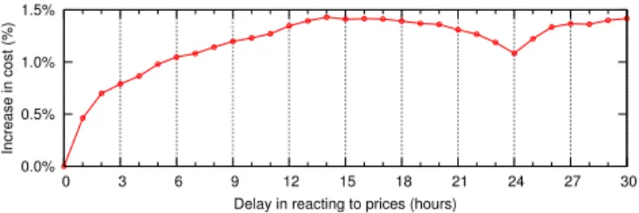
Not reacting immediately to price changes noticeably re-duces overall savings. In our simulations we were conserva-tive and assumed that there was a one hour delay between the market setting new prices and the system propagating new routes.

Figure 20 shows how increasing the reaction delay impacts prices. First, note the initial jump, between an immediate reaction and a next-hour reaction. This implies achievable savings will exceed what we have calculated for systems that can update their routes in less than an hour. Further, note the local minima at the 24 hour mark. This is probably because market prices can be correlated for a given hour from one day to the next.

The increase in cost is substantial. With the (65% idle, 1.3 PUE) energy model, the maximum savings is around 5% (see figure 15). So a subsequent increase in cost of 1% would eliminate a large chunk of the savings.

0.0% 0.5% 1.0% 1.5% 0 3 6 9 12 15 18 21 24 27 30 Increase in cost (%)

Delay in reacting to prices (hours)

Figure 20: Impact of price delays on electricity cost for a (65% idle, 1.3 PUE) model, with a distance threshold of 1500km.

7.

ACTUAL ELECTRICITY BILLS

In this paper, we assume that power bills are based on hourly market prices and on energy consumption. Addi-tionally, we assume that the decisions of server operators will not affect market prices.

The strength of this approach is that we can use price data to quantify how much money would have been saved. However, in reality, achieving these savings would probably require a renegotiation of existing utility contracts. Further-more, rather than passively reacting to spot prices, active participation opens up additional possibilities.

Existing Contracts. It is safe to say that most current contractual arrangements would reduce the potential sav-ings below what our analysis indicates. That said, server operators should be able to negotiate deals that allow them to capture at least some of this value.

Wholesale-indexed electric billing plans are becoming in-creasingly common throughout the US. This allows small companies that do not participate directly in the wholesale market to take advantage of our techniques. This billing structure appeals to electricity providers since risk is trans-ferred to consumers. For example, in the mid-west RTO Commonwealth Edison offers a Real-Time Pricing program [26]. Customers enrolled in it are billed based on hourly consumption and corresponding wholesale PJM-MISO loca-tional market prices.

Companies, such as Akamai, renting space in co-location facilities will almost certainly have to negotiate a new billing structure to get any advantage from our approach. Most co-location centers charge by the rack, each rack having a maximum power rating. In other words, a company like Akamai pays for provisioned power, and not for actual power used. We speculate that as energy costs rise relative to other costs, it will be in the interest of co-location owners to charge based on consumption and possibly location. There is evi-dence that bandwidth costs are falling, but energy costs are not. Even if new kinds of contracts do not arise, server op-erators may be able to sell their load-flexibility through a side-channel like demand response, as discussed below, by-passing inflexible contracts.

Selling Flexibility. Distributed systems with energy elastic clusters can be more flexible than traditional con-sumers: operators can quickly and precipitously reduce power usage at a location (by suspending servers, and routing re-quests elsewhere). Market mechanisms already exist that would allow operators to value and sell this flexibility.

Some RTOs allow energy users to bid negawatts (nega-tive demand, or load reductions) into the day-ahead market auction. This is believed to moderate prices.

Alternatively, customers could enroll in triggered demand response programs, agreeing to reduce their power usage in response to a request by the grid operators. Load reduction requests are sent out when electricity demand is high enough to put grid reliability at risk, or rising demand requires the imminent activation of expensive/unreliable generation as-sets. The advance notice given by the RTO can range from days to minutes. Participating customers are compensated based on their flexibility and load. Demand-response vari-ants exist in every market we cover in this paper.

Even consumers using as little as 10kW (a few racks) can participate in such programs. Consumers can also be aggre-gated into large blocs that reduce load in concert. This is the approach taken by EnerNOC, a company that collects many consumers, packages them, and sells their aggregate ability to make on-demand reductions. A package of hotels would, for example, reduce laundry volume in sync to ease power demand on the grid.

The good thing about selling flexibility as a product, is that this is valued even where wholesale markets do not exist. It even works if price-differentials don’t exist (e.g. fixed price contracts or in highly regulated markets).

However, we have ignored the demand side. How do op-erators construct bids for the day-ahead auctions if they don’t know next-day client demand for each region? What happens when operators are told to reduce power consump-tion at a locaconsump-tion, when there is a concentraconsump-tion of active clients nearby? In systems like Akamai, demand is gener-ally predictable, but there will be heavy traffic days that are impossible to predict.

There is anecdotal evidence that data centers have partic-ipated in demand response programs [3]. However, the ap-plicability of demand response to single data centers is not widely accepted. Participating data centers may face addi-tional downtime or periods of reduced capacity. Conversely, when we look at large distributed systems, participation in such programs is attractive. Especially when the barriers to entry are so low—only a few racks per location are needed to construct a multi-market demand response system.

8.

FUTURE WORK

Some clear avenues for future work exist.

Implementing Joint Optimization. Existing systems already have frameworks in place that engineer traffic to optimize for bandwidth costs, performance, and reliability. Dynamic energy costs represent another input that should be integrated into such frameworks.

RTO Interaction. Service operators can interact with RTOs in many ways. This paper has proposed a relatively passive approach in which operators monitor spot prices and react to favourable conditions. As we discussed in section 7, there are other market mechanisms in place that service operators may be able to exploit. The optimal market par-ticipation strategy is unclear.

Weather Differentials. Data centers expend a lot of energy running air cooling systems, up to 25% of total en-ergy. In modern systems, when ambient temperatures are low enough, external air can be used to radically reduce the power draw of the chillers. At the same time, weather temperature differentials are common. This suggests that significant energy savings can be achieved by dynamically

routing requests to sites where the heat generated by serv-ing the request is most inexpensively removed. Unlike price differentials, which reduce cost but not energy, routing re-quests to cooler regions may be able to reduce both.

Environmental Cost. Rather than attempting to min-imize the dollar cost of the energy consumed, a socially re-sponsible service operator may instead choose to use an envi-ronmental impact cost function. The envienvi-ronmental impact of a service is time-varying. An obvious cost function is the carbon footprint of the energy used. In grids that aggre-gate electricity from diverse providers, the footprint varies depending upon what generating assets are active, whether power plants are operating near optimal capacity and what mixture of fuels they are currently using. The variation oc-curs at multiple time scales, e.g., seasonal (is there water to power hydro systems), weekly (what are the relative prices of various fossil fuels), and hourly (is the wind blowing or the tide going out). Additionally, carbon is not the only pol-lutant. For instance, power plants are the primary station-ary sources of nitrogen oxide in the US. Due to variations in weather and atmospheric chemistry, the timing and location of NOxreductions determine their effectiveness in reducing

ground-level ozone [27].

9.

CONCLUSION

The bounds derived in this paper should not be taken too literally. Our cost and traffic models are based on actual data, but they do incorporate a number of simplifying as-sumptions. The most relevant assumptions are probably (1) that operators can do better by buying electricity on the open market than through negotiated long-term contracts, and (2) that the variable energy costs associated with ser-vicing a request are a significant fraction of the total costs. Despite these caveats, it seems clear that the nature of ge-ographical and temporal differences in the price of electricity offers operators of large distributed systems an opportunity to reduce the cost of servicing requests. It should be pos-sible to augment existing optimization frameworks to deal with electricity prices.

Acknowledgements

We thank our shepherd Jon Crowcroft and the anonymous reviewers for their insightful comments. We also thank John Parsons, Ignacio Perez-Arriaga, Hariharan Shankar Rahul, and Noam Freedman for their help. This work was sup-ported in part by Nokia, and by the National Science Foun-dation under grant CNF–0435382.

10.

REFERENCES

[1] R. H. Katz, “Tech Titans Building Boom,” IEEE Spectrum, February 2009.

[2] K. G. Brill, “The Invisible Crisis in the Data Center: The Economic Meltdown of Moore’s Law,” white paper, Uptime Institute, 2007.

[3] “Server and Data Center Energy Efficiency,” Final Report to Congress, U.S. Environmental Protection Agency, 2007.

[4] Google Inc., “Efficient Computing: Data Centers.” http://www.google.com/corporate/green/ datacenters/.

[5] X. Fan, W.-D. Weber, and L. A. Barroso, “Power Provisioning for a Warehouse-sized Computer,” in ACM International Symposium on Computer Architecture, 2007.

[6] L. A. Barroso and U. H¨olzle, “The Case for Energy Proportional Computing,” IEEE Computer, 2007. [7] D. Meisner, B. T. Gold, and T. F. Wenisch,

“PowerNap: Eliminating Server Idle power,” in ACM ASPLOS, 2009.

[8] G. Chen, W. He, J. Liu, S. Nath, L. Rigas, L. Xiao, and F. Zhao, “Energy-Aware Server Provisioning and Load dispatching for Connection-Intensive Internet Services,” in NSDI, 2008.

[9] VMware DRS: Dynamic Scheduling of System Resources.

[10] N. Tolia, Z. Wang, M. Marwah, C. Bash, P. Ranganathan, and X. Zhu, “Delivering Energy Proportionality with Non Energy-Proportional Systems – Optimizing the Ensemble,” in HotPower, 2008.

[11] N. Joukov and J. Sipek, “GreenFS: Making Enterprise Computers Greener by Protecting Them Better,” in ACM Eurosys, 2008.

[12] Randy Shoup, “Scalability Best Practices: Lessons from eBay.”

[13] J. Markoff and S. Hansell, “Hiding in Plain Sight, Google Seeks an Expansion of Power,” the New York Times, June 2006.

[14] Microsoft Environmental Sustainability group, “Q&A with Rob Bernard,” Video.

[15] “61 Billion Searches Conducted Worldwide in August,” Press Release, comScore Inc.

[16] United States Department of Energy, Official Statistics. http://www.eia.doe.gov.

[17] World Bank, “World Development Indicators Database.”

[18] Platts, “Day-Ahead Market Prices,” in Megawatt Daily, McGraw-Hill. 2006-2009.

[19] United States Federal Energy Regulatory Commission, Market Oversight. http://www.ferc.gov.

[20] Midwest ISO, “Market Concepts Study Guide,” 2005. [21] P. L. Joskow, “Markets for Power in the United States:

an Interim Assessment,” Aug. 2005.

[22] Severin Borenstein, “The Trouble With Electricity Markets: Understanding California’s Restructuring Disaster,” Journal of Economic Perspectives, 2005. [23] L. Hadsell and H. A. Shawky, “Electricity Price

Volatility and the Marginal Cost of Congestion: An Empirical Study of Peak Hours on the NYISO Market,” The Energy Journal.

[24] U. H¨olzle, “Powering a Google Search,” Official Google Blog, Jan. 2009.

[25] J. Chabarek, J. Sommers, P. Barford, C. Estan, D. Tsiang, and S. Wright, “Power Awareness in Network Design and Routing,” INFOCOM, 2008. [26] “Commonwealth Edison.” www.comed.com. [27] K. C. Martin, P. L. Joskow, and A. D. Ellerman,

“Time and Location Differentiated NOX Control in Competitive Electricity Markets Using Cap-and-Trade Mechanisms,” April 2007.