Data Completion Problems Solved as Nash Games

HAL Id: hal-00648712

https://hal.inria.fr/hal-00648712

HAL is a multi-disciplinary open access

archive for the deposit and dissemination of sci-entific research documents, whether they are pub-lished or not. The documents may come from teaching and research institutions in France or abroad, or from public or private research centers.

L’archive ouverte pluridisciplinaire HAL, est destinée au dépôt et à la diffusion de documents scientifiques de niveau recherche, publiés ou non, émanant des établissements d’enseignement et de recherche français ou étrangers, des laboratoires publics ou privés.

Abderrahmane Habbal, Moez Kallel

To cite this version:

Abderrahmane Habbal, Moez Kallel. Data Completion Problems Solved as Nash Games. Journal of Physics: Conference Series, IOP Publishing, 2012, 386, �10.1088/1742-6596/386/1/012004�. �hal-00648712�

Data completion problems solved as Nash games

1_{Laboratoire J.A.Dieudonn´e, Universit´e de Nice & INRIA, France} 2_{Laboratoire LAMSIN-ENIT & IPEIT, Universit´e de Tunis, Tunisia}

E-mail:[email protected] and [email protected]

Abstract. We consider the Cauchy problem for an elliptic operator, formulated as a Nash game. The over specified Cauchy data are split among two players : the first player solves the elliptic equation with the Dirichlet part of the Cauchy data prescribed over the accessible boundary, and a variable Neumann condition (which we call first player’s strategy) prescribed over the inaccessible part of the boundary. The second player makes use correspondingly of the Neumann part of the Cauchy data, with a variable Dirichlet condition prescribed over the inaccessible part of the boundary. The first player then minimizes the gap related to the non used Neumann part of the Cauchy data, and so does the second player with a corresponding Dirichlet gap. The two costs are coupled through a distributed field gaps. We prove that there exists always a unique Nash equilibrium, which turns out to be the reconstructed data when the Cauchy problem has a solution. We also prove that the completion algorithm is stable with respect to noise. Some numerical 2D and 3D experiments are provided to illustrate the efficiency and stability of our algorithm.

1. Introduction

We consider the following elliptic Cauchy problem :

     ∇.(k∇u) = 0 in Ω u = f on Γc k∇u.ν = Φ on Γc (1)

where_{Ω is a bounded open domain in R}d(d = 2, 3) with a sufficiently smooth boundary ∂Ω

composed of two connected disjoint componentsΓc andΓi. The parameters k, f andΦ are

given functions, ν is the unit outward normal vector on the boundary. The Dirichlet data f

and the Neumann dataΦ are the so-called Cauchy data, which are known on the accessible

partΓc of the boundary ∂Ω and the unknown field u is the Cauchy solution.

The above Cauchy problem is also known as a data completion problem, where the data to be recovered, or missing data, are u|Γi and k∇u.ν|Γi, which are determined as soon as

one knows u in the whole domain Ω. Cauchy problem is a prototype of Inverse Boundary

Value Problems (IBVP), which model a wide field of applications ranging from medical imaging to detection and nondestructive testing, and addressing quasi exhaustively all the

fields of physics, from electromagnetism to acoustics, fluid and structural mechanics (see e.g. [8, 9, 12, 16]).

Classically, IBVP are known to be ill-posed. For instance, the solution of Cauchy problem does not always exist for any pair of data(f, Φ), and if such a solution exists, it does

not always depend continuously on the data (Hadamard’s ill-posedness, see [20]). The Cauchy data(f, Φ) are called compatible (or consistent) if the corresponding Cauchy problem (1) has

a solution (it is then unique thanks to classical continuation arguments). Ill-posedness in the sense of Hadamard makes classical numerical methods usually inappropriate because they are unstable, and there is a need for carefully stabilized dedicated computational methods, sometimes by regularizing (through reformulation of) the Cauchy problem itself. Readers may refer to a wide literature dealing with the efficient numerical solution of elliptic Cauchy problems, e.g. [3, 13, 14, 15, 17, 22] and, dealing with the ill-posedness for the Cauchy problem, [2, 10, 11] among many others.

Our purpose is to introduce an original method to solve the Cauchy problem, based on a game theory approach. We first recall in section 2 an optimal control formulation to solve the Cauchy problem used in [1]. We then show in section 3 that the control formulation naturally leads to a Nash game of static nature with complete information, which involves a Dirichlet gap and a Neumann gap costs. The existence and uniqueness of the Nash equilibrium is proved, and when the Cauchy solution exists, it turns out that the Nash equilibrium is exactly the pair of missing data of the Cauchy problem; afterwards, we end the section with a convergence result with respect to noisy data. Section 4 is devoted to sensitivity and implementation aspects, used to lead some numerical experiments. The numerical results are presented in section 5 to illustrate the efficiency of the present game-based approach. We end the paper by some concluding remarks.

The reader interested in some PDE’s oriented applications of game theory may refer to [18, 19], and refer to [7, 23, 24] for a general introduction and proof of convergence of computational methods for Nash equilibria, and finally refer to [4, 5, 6] for a study of alternating algorithms which are in close link with our present approach.

2. An optimal control formulation of the Cauchy problem

We assume that the boundary ∂Ω and the data k, Φ and f are smooth enough, at least ∂Ω is

of class C2 and(Φ, f ) ∈ L2_(Γ

c) × H1(Γc). In this case, the Cauchy solution u, if it exists,

belongs to the space H3/2(Ω).

In [1], the authors formulate the Cauchy problem (1) as an optimal control one. The setting is as follows :

For given η ∈ L2_(Γ

i) and τ ∈ H1(Γi), let us define u1(η) and u2(τ ) as the unique

solutions in H1(Ω) of the following elliptic boundary value problems :

(SP 1)      ∇.(k∇u1) = 0 in Ω u1 = f on Γc k∇u1.ν = η on Γi (SP 2)      ∇.(k∇u2) = 0 in Ω u2 = τ on Γi k∇u2.ν = Φ on Γc (2)

The optimization problem amounts to minimize, among all Neumann-Dirichlet pairs

(η, τ ) ∈ L2_(Γ

i) × H1(Γi), the following “Neumann-gap” cost :

J1(η, τ ) = 1(η, τ, u1(η), u2(τ )) = 1 2 Z Γc (k∇u1.ν−Φ)2dΓc + 1 2 Z Γi (u1−u2)2dΓi.(3)

The authors in [1] proved that when the Cauchy problem (1) has a solution, then solving it is equivalent to solving the minimization problem

min

(η,τ )∈L2

(Γi)×H1(Γi)

J1(η, τ ). (4)

They also proved that the functionalJ1 is twice Fr´echet differentiable and strictly convex.

The same conclusions above hold when a “Dirichlet-gap” cost is considered :

J2(η, τ ) = 2(η, τ, u1(η), u2(τ )) = 1 2 Z Γc (u2 − f )2dΓc + 1 2 Z Γi (u1 − u2)2dΓi. (5)

Let us remark that the choice of the functional spaces L2(Γi) and H1(Γi) as control

spaces allows for the cost functions to be well defined, since we know from classical a priori estimates for elliptic boundary systems that u1 and u2 belong to the space H3/2(Ω) (so that

the normal derivatives k∇u1.ν and k∇u2.ν belong to L2(Γc), the natural space for the flux

dataΦ).

3. A Nash game formulation of the Cauchy problem

From the previous section, we remark that, formulated in the game theory language, the Neumann and Dirichlet controls η and τ do cooperate to minimize either the Neumann-gap or the Dirichlet-gap costs. These two controls could as well cooperatively minimize any convex combination of the two costsJ1andJ2.

Now, the fields u1(η) and u2(τ ) are aiming at the fulfillment of a possibly antagonistic

goals, namely minimizing the Neumann gap kk∇u1.ν − ΦkL2_(Γ

c) and the Dirichlet gap

ku2−f kL2

(Γc). This antagonism is intimately related to Hadamard’s ill-posedness character of the Cauchy problem, and rises as soon as one requires that u1and u2coincide, which is exactly

what the coupling term ku1 − u2kL2

(Γi) is for. Thus, one may think of an iterative process which minimizes in a smart fashion the three terms, namely Neumann-Dirichlet-Coupling terms.

Let us define the following two costs : for any η∈ L2_(Γ

i) and τ ∈ H1(Γi), J1(η, τ ) = 1 2 Z Γc (k∇u1.ν− Φ)2dΓc + α 2 Z Ω (u1− u2)2dΩ (6) J2(η, τ ) = 1 2 Z Γc (u2− f )2dΓc + α 2 Z Ω (u1− u2)2dΩ (7)

where the fields u1(η) and u2(τ ) are the unique solutions to (SP1) and (SP2), respectively.

Differently from the definition ofJ1,J2 above, the coupling term is now distributed over the

whole domainΩ and α is a given positive parameter (e.g. α = 1).

One may consider a decomposition-like method where the variable η is used to minimize the Neumann gap + coupling term, in other words J1, and τ is used to minimize the Dirichlet

gap + coupling term, which defines J2. Such a method fits into the area of mathematical

games.

We shall say that there are two players, referred to as player 1 or Neumann-gap, and player 2 or Dirichlet-gap. Player 1 controls the strategy variable η, and player 2 controls the strategy variable τ . Each of the two players tries to minimize its own cost, namely J1 for

player 1, and J2 for player 2. As classical, the fact that each player controls only his own

strategy, while there is a strong dependance of each player’s cost on the joint strategies(η, τ )

justifies the use of the game theory framework (and terminology), a natural setting which may be used to formulate the negotiation between these two costs.

In order to be consistent with the initial formulation of the Cauchy problem, the relevant game theoretic framework to deal with is a static with complete information one. In this case, a commonly used solution concept (roughly speaking, in the game vocabulary, a rational and stable one) is the one of Nash Equilibria, defined as follows :

Definition 1 A pair(ηN, τN) ∈ L2(Γi) × H1(Γi) is a non-cooperative Nash equilibrium (NE)

if      J1(ηN, τN) ≤ J1(η, τN), ∀η ∈ L2(Γi), J2(ηN, τN) ≤ J2(ηN, τ), ∀τ ∈ H1(Γi). (8)

It is of importance to notice that the present game has a separable structure. Indeed, the players criteria are formed of individual costs, the Neumann-gap depending only on η for player 1 and the Dirichlet-gap, depending only on τ for player 2, plus a common coupling cost which depends on both η and τ . Such game belongs to a family referred to as Inertial Nash Equilibration Processes in [5]. The game separable structure is crucial in our study, and we shall exploit it to prove that there exists a unique Nash equilibrium, which is shown to be the missing data when a Cauchy solution does exist. Based upon this structure of the criteria, we shall also establish a convergence result with respect to noisy data.

As a preliminary, let us remark that the field u1(η) is affine with respect to η, and so is

the field u2(τ ) w.r.t. the variable τ . Thus, the functions J1 and J2 are quadratic. Following

e.g. [1], it is an easy exercise to compute their second order differentials.

Let us consider the case of J1, the one of J2follows the same steps. First, notice that we

can set

u1(η) = u1,0(η) + u1,f

where u1,0(η) solves the boundary value problem :

     ∇.(k∇u1,0) = 0 in Ω u1,0 = 0 on Γc k∇u1,0.ν = η on Γi (9)

Then it is easy to compute the second order differential of J1 w.r.t. η in any direction

ψ ∈ L2_(Γ i) which reads : (d2J1(η, τ ).ψ, ψ) = Z Γc (k∇u1,0(ψ).ν)2dΓc + α Z Ω (u1,0(ψ))2dΩ.

It is immediate that if(d2_J

1(η, τ ).ψ, ψ) = 0 then u1,0(ψ) = 0, hence ψ = 0.

Indeed, strict convexity of J1 and J2 holds w.r.t. the pair(η, τ ) as well. On the contrary,

we shall see that partial ellipticity (or coerciveness) of the costs holds while it does not w.r.t. the pair(η, τ ), precisely because of the coupling term.

Let us again focus on the case of J1. If partial ellipticity fails, then there exists a sequence

(ψn) ⊂ L2(Γi) such that

|ψn|L2

(Γi) = 1 and (d

2_J

1(η, τ ).ψn, ψn) → 0 when n → +∞. (10)

Thanks to the classical regularity results and a priori estimates for elliptic BVPs, one gets

ku1,0(ψn)k_H3

2_(Ω) ≤ |ψn|L

2_(Γ

i)

So, up to a subsequence, (u1,0(ψn)) weakly converges in H

3

2(Ω). By invoking the

Rellich-Kondrachov theorem, the sequence strongly converges to some z ∈ H1_{(Ω). Since (u}

1,0(ψn))

strongly converges to zero in L2(Ω) thanks to (10), one has z = 0. Now, thanks to the

continuity of the normal trace operator, one has ψn → k∇z.ν (= 0) in H−

1

2(Γ

i), which is

in contradiction with|ψn|L2

(Γi) = 1. We summarize the above preliminary results in the Proposition 1 The partial mapping η → J1(η, τ ) (resp. τ → J2(η, τ )) is a quadratic strongly

convex functional over L2(Γi) (resp. H1(Γi)).

It is important to notice that the partial ellipticity property of η → J1(η, τ ) holds

uniformly w.r.t. τ , and conversely for J2. It allows us to bound the strategy spaces if necessary.

Following [5], let us introduce the functional L(η, τ ) as follows :

L(η, τ ) = 1 2 Z Γc (k∇u1(η).ν−Φ)2dΓc+ 1 2 Z Γc (u2(τ )−f )2dΓc+ α 2 Z Ω (u1(η)−u2(τ ))2dΩ.(11)

It is easy to check that L is strictly convex, and that any minimum of L is a Nash equilibrium and conversely, thanks to the separable structure of the present game (consider the necessary optimality conditions). We conclude that if a Nash equilibrium exists, then it is unique.

The existence of a Nash equilibrium (ηN, τN) ∈ L2(Γi) × H1(Γi), id est a pair which

fulfills (8), is obtained by a direct application of the Nash theorem : since strategy variables belong to Hilbert spaces, the uniform partial ellipticity of the costs allows for the choice of -large enough- closed bounded balls, which are then weakly compact convex sets, then continuity of the convex costs yields the weak lower semi-continuity over the so-defined balls. Finally, remark that if a Cauchy solution u does exist, then by setting ηC = k∇u.ν|Γiand

τC = u|Γi, one has immediately L(ηC, τC) = 0, since thanks to the uniqueness of the Cauchy solution, u1(ηC) = u2(τC) = u. In this case, one has that (ηC, τC) is the minimum of the

nonnegative functional L, and so it is also the Nash equilibrium(ηN, τN).

We summarize the above results in the following:

Proposition 2 Consider the Nash game defined by (6)-(7)-(8).

(i) There always exists a unique Nash equilibrium(ηN, τN) ∈ L2(Γi) × H1(Γi) . It is also

(ii) When the Cauchy problem has a solution u, then u1(ηN) = u2(τN) = u, and (ηN, τN)

are the missing data, namely ηN = k∇u.ν|Γi and τN = u|Γi.

Let us now consider the case of noisy data. We assume that there exists a pair of

compatible data (f, Φ), and denote by u the corresponding Cauchy solution. We consider

a family of not necessarily compatible data(fδ_,Φδ_{) ∈ H}1_(Γ

c) × L2(Γc) such that : kfδ− f k2_H1 (Γc)+ kΦ δ_{− Φk}2 L2 (Γc) ≤ δ 2_{. (12)} For given (η, τ ) ∈ L2_(Γ

i) × H1(Γi), the fields uδ1(η) and uδ2(τ ) are solution of the

respective problems :      ∇.(k∇uδ 1) = 0 in Ω uδ₁ = fδ _{on Γ} c k∇uδ 1.ν = η on Γi      ∇.(k∇uδ 2) = 0 in Ω uδ₂ = τ on Γi k∇uδ 2.ν = Φδ on Γc (13)

We define the associated cost functionals :

J₁δ(η, τ ) = 1 2 Z Γc (k∇uδ₁.ν− Φδ)2dΓc + α 2 Z Ω (uδ₁− uδ₂)2dΩ (14) J₂δ(η, τ ) = 1 2 Z Γc (uδ₂− fδ)2dΓc + α 2 Z Ω (uδ₁− uδ₂)2dΩ (15)

The functions J₁δand J₂δhave the properties declined in Proposition-1, so there exists a unique

corresponding Nash equilibrium(ηδ

N, τNδ) ∈ L2(Γi) × H1(Γi).

One may ask if, when δ→ 0, the Nash equilibrium (ηδ

N, τNδ) does converge to the missing

data (k∇u.ν|Γi, u|Γi) or, in other words, do the fields u

δ

1(ηδN) and uδ2(τNδ) converge to the

Cauchy solution u?

Let us again use the notation ηC = k∇u.ν|Γi and τC = u|Γi the Cauchy missing data, and introduce the auxiliary functions z₁δ = uδ

1(ηC) − u and zδ2 = uδ2(τC) − u. Then, using the

continuity of the trace operator from H32(Ω) onto H1(∂Ω), and the continuity of the normal trace operator from H32(Ω) onto L2(∂Ω), it is easy to show that (obvious notation is used to define Lδ from its definition in (11)) :

Lδ(ηC, τC) ≤ (1 + α)(kz1δk2_H3

2_(Ω) + kz

δ 2k2_H3

2_(Ω))

Using classical a priori estimates (z₁δfulfills the elliptic equation with non-homogeneous Dirichlet condition, and z₂δ a one with non-homogeneous Neumann condition), one gets :

Lδ(ηC, τC) ≤ (1 + α) ³ kfδ− f k2_H1 (Γc)+ kΦ δ_{− Φk}2 L2 (Γc) ´ ≤ (1 + α)δ2.(16)

We have previously seen that the Nash equilibrium(ηδ

N, τNδ) is also the unique minimum

of Lδ, thus we have :

J₁δ(η_Nδ, τ_Nδ) ≤ Lδ(η_Nδ, τ_Nδ) ≤ Lδ(ηC, τC) ≤ (1 + α)δ2 (17)

and J₂δ(ηδ

N, τNδ) ≤ (1 + α)δ2 as well. Now, since the mapping η → J1δ(η, τ ) is coercive,

uniformly in τ (and in δ), and since the same corresponding property holds for τ → Jδ 2(η, τ ),

we obtain that the sequence (ηδ

N) is uniformly bounded in L2(Γi) and (τNδ) is uniformly

bounded in H1(Γi). Up to a subsequence, we have from one part that ηNδ converges weakly

to some η_N0 ∈ L2_(Γ

i), strongly in the H−

1

2(Γ

i) topology. From other part, the sequence τNδ

converges weakly to some τ_N0 ∈ H1_(Γ

i), strongly in the H

1

2(Γ

i) topology. Since the sequence

fδstrongly converges to f in H1(Γc) and Φδstrongly converges toΦ in L2(Γc), we conclude

that the sequences uδ₁(ηδ

N) and uδ2(τNδ), which are the solutions to equations (13), strongly

converge in H1(Ω) to respectively u1(η0N) and u2(τN0) which are the unique solutions to the

respective equations:              ∇.(k∇u1) = 0 in Ω u1 = f on Γc k∇u1.ν = ηN0 on Γi              ∇.(k∇u2) = 0 in Ω u2 = τN0 on Γi k∇u2.ν = Φ on Γc (18)

Taking δ → 0 in (17) yields that (k∇uδ

1.ν− Φδ) strongly converges to 0 in L2(Γc), which

means that (k∇uδ

1.ν) strongly converges to Φ in L2(Γc) so a fortiori in H−

1

2(Γ

c). Hence,

k∇u1.ν = Φ over Γc. Thanks to the uniqueness of the Cauchy problem, we conclude that

u1 = u. The same reasoning applied to the coupling term in J1δwould directly yield u1 = u2

and thanks to the equations (18), the two fields are equal to the Cauchy solution u as well.

Finally, we have proved that the sequence (ηδ

N) strongly converges in L2(Γi) to η0N =

ηC = k∇u.ν|Γi and that the sequence(τ

δ

N) strongly converges in H1(Γi) to τN0 = τC = u|Γi. Proposition 3 Assume there exists a unique Cauchy solution u ∈ H1_{(Ω) for a given}

compatible pair of data (f, Φ) ∈ H1_(Γ

c) × L2(Γc). Let (fδ,Φδ) ∈ H1(Γc) × L2(Γc) be

any sequence of noisy data such that

kfδ− f k2_H1_(Γ c)+ kΦ δ_{− Φk}2 L2_(Γ c) ≤ δ 2_.

Then, the Nash game corresponding to the costs J₁δ and J₂δ defined by (14)-(15) has a unique Nash equilibrium(ηδ

N, τNδ) ∈ L2(Γi) × H1(Γi) which strongly converges, as δ → 0,

to the Cauchy missing data(k∇u.ν|Γi, u|Γi).

Moreover, the solutions to the equations (13), respectively uδ₁(ηδ

N) and uδ2(τNδ), strongly

converge in H1(Ω) to the Cauchy solution u.

4. Numerical procedure

From the computational viewpoint, in [5] the authors propose an alternating minimization algorithm to compute the Nash Equilibrium by means of the following iterative process :

Let(η0_{, τ}0_{) be a given initial state ;}

     η(k+1) = argmin_η{J1(η, τ(k)) + β₂ R Γi(η − η (k)₎2_dΓ i}, τ(k+1)_{= argmin} τ{J2(η(k+1), τ) + β₂ R Γi(τ − τ (k)₎2_dΓ i}, (19)

where β is a given positive parameter (e.g. β = 1).

In the cited reference, the convergence of the alternating algorithm above is proved, under suitable assumptions which also hold in our case, see Proposition 1.

Our algorithm is written as follows :

Set k= 0. Starting from an initial guess S(0) _{= (η}(0)_{, τ}(0)_):

Step 1: Compute η(k), which solvesminηJ1(η, τ(k));

Step 2: Compute τ(k), which solvesminτJ2(η(k+1), τ);

Step 3: Set S(k+1) = (η(k+1)_{, τ}(k+1)_{) = t (η}(k)_{, τ}(k)_{) + (1 − t) (η}(k)_{, τ}(k)_{), 0 < t < 1.}

Redo (Step 1) until the sequence S(k) converges. As a stopping criterion we choose a

classical one, the first k such that,

kS(k+1)_{− S}(k)_{k ≤ ǫ,}

where ǫ is given small enough parameter.

It is easy to show that the above procedure is equivalent to the algorithm (19) as soon as one uses a fixed step gradient method to solve the partial optimization problems in Step 1 and

Step 2 above. For numerical problem, we used the discetized version which was proved to

converge in [24].

To this end, the gradients may be efficiently computed by means of an adjoint state method. Let us define the following Lagrangian:

L(η, τ, τ∗_{, u} 1, u2, λ1, λ2) = α 2 Z Ω (u1− u2)2dΩ + 1 2 Z Γc (k∇u1.ν− Φ)2dΓc + Z Ω k∇u1.∇λ1dΩ − Z Γi ηλ1dΓi + Z Ω k∇u2.∇λ2dΩ − Z Γc Φλ2dΓc + Z Γi (u2− τ )τ∗dΓi (20) where (η, τ ) ∈ L2_(Γ i) × H1(Γi), (u1, u2, λ1, λ2) ∈ H 3 2(Ω) × H 3 2(Ω) × W 1 × W2 and τ∗ _{∈ L}2_(Γ

i), where the latter two spaces are given by :

W1 = {v ∈ H 3 2(Ω) such that v| Γc = 0} and W2 = {v ∈ H 3 2(Ω) such that v| Γi = 0}. The Lagrangian is used to compute the gradients∇ηJ1 and∇τJ2 :

Proposition 4 We have the following two partial derivatives:

                   ∂J1 ∂η (η, τ )ξ = − Z Γi λ1ξ dΓi, for all ξ ∈ L2(Γi)

where λ1 ∈ W1solves the adjoint problem:

Z Ω k∇λ1.∇γ dΩ = −α Z Ω (u1− u2)γ dΩ − Z Γc (k∇u1.ν− Φ)(k∇γ.ν) dΓc, γ ∈ W1 (21)

and                          ∂J2 ∂τ (η, τ )h = Z Γi (k∇λ2.ν)h dΓi, h∈ H1(Γi)

where λ2 ∈ W2solves the adjoint problem:

     ∇.k∇λ2 = α (u1− u2) in Ω k∇λ2.n = f − u2 on Γc λ2 = 0 on Γi (22) 5. Numerical results

The computational methodology used to illustrate the efficiency of the present approach is classical. All experiments are performed on a Personal Computer and all the partial differential equations are numerically solved using FreeFem++ [21], a Finite Element based free software. In order to obtain accurate approximations of the normal derivatives of u1 and

of λ2, the dual Raviart-Thomas mixed finite elements are used.

We consider a domain Ω defined as the open bounded set delimited by two concentric

circles in 2D test-cases, or two concentric spheres in 3D test-cases. The inner boundary plays the role ofΓi, where the trace and normal derivative are missing, and the outer one plays the

one ofΓcwhere the latter information is over specified.

We then consider explicit well-known analytical solutions, generically denoted by u, which are harmonic inside the domainΩ, and set the trace and normal derivative of u over Γc

as being the measured data f = u|Γc andΦ = (k∇u.ν)|Γc. We sometimes refer to these data as temperature and flux (with obvious interpretation).

In order to test the robustness of the proposed method we add a white noise to the temperature f and the heat fluxΦ as follows:

fσ = u + σw1 and Φσ = k∇u.ν + σw2, on Γc, (23)

where σ denotes the noise level relative to k.kL2

(Γc) of u and k∇u.ν respectively, whereas

(w1, w2) are normelly distributed random functions.

Our algorithm performs a denoising task on the noisy prescribed Cauchy data fσ andΦσ_.

For instance, let us denote by(τσ

N, ηNσ) the Nash equilibrium associated to the latter noisy over

specified data. Then, the pair of optimal solutions (u2(τN)|Γc,(k∇ ˜u1.ν)|Γc) may be viewed as regularized Cauchy data obtained from the noisy Cauchy data, whereu˜1 is the solution of

     ∆ ˜u1 = 0 in Ω, ˜ u1 = u2(τN) on Γc, k∇ ˜u1.ν= ηN on Γi. (24)

We present numerical results which illustrate the stability of our method with respect to noisy data, as well as an example of the noise deblurring property underlined above. The presented graphics are related to the profiles over Γi of the Dirichlet and Neumann missing

the fields and to the missing profiles, as a function of iterations and for different noise levels. We also present a stationarity history for the Nash overall computation iterations.

The computation of the Nash equilibrium is performed as described in section 4, where the partial optimization tasks of Step-1 and Step-2 use a fixed line-search gradient method. Here, it is sufficient to carry out only few iterations in the optimization process in each step. A second formulation would be obtained, if we assume that the players compute not sequentially, but in parallel with step-1, in the Step-2 we compute τ(k)which solvesminτJ2(η(k), τ).

An arbitrary initial guess such as S(0) = (η(0)_{, τ}(0)_{) = (0, 0) is chosen to start-up the}

algorithm, the physical function k takes the constant value 1 in Ω, and the parameters α

(weight of the coupling term in the costs) and t (relaxation parameter in the computation of

Nash equilibrium) are set to α= 1 and t = 0.25.

5.1. Two 2D test-cases

We consider an annular domainΩ with circular boundary components ΓiandΓc, both centered

at(0, 0) and with radii Ri = 0.6 and Rc = 1, respectively.

Test-case A. The first 2D experiment is related to a smooth case. The -artificial- Cauchy

data f andΦ are defined as respectively the trace and normal derivative, over the circle Γc, of

the harmonic function :

u(x, y) = excos(y).

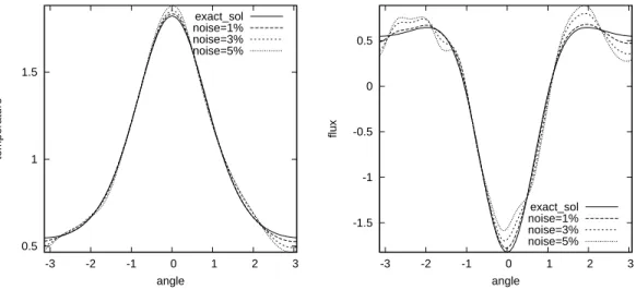
In figure-1, the missing data τN and ηN are presented at convergence of the algorithm

(19) dedicated to the computation of the Nash equilibrium, for different noise levels σ. The obtained Dirichlet as well as Neumann profiles show remarkable stability with respect to noise.

Test-case B. The second 2D experiment is related to the singular function :

u(x, y) = Re( 1

z− a), where z = x + iy.

In this case, the singularity source, located at a = (0.5, 0), is in the vicinity of the circle Γi, and reconstruction of the solution over this boundary is a numerically challenging task,

particularly in the case of noisy data.

The results in figure-2 show again the stability of our method. The profile shape is well captured including the localization of the singularity peak, whose magnitude is however underestimated for the trace as well as for the normal derivative.

Finally, the denoising effect, through computing the Nash equilibrium and solving of equation (24), is actually observed in figure-3 for a noise level of 5%.

5.2. Two 3D test-cases

As for the 2D case, we consider a thick spherical shell domainΩ with boundary components

ΓiandΓc, which are two spheres both centered at(0, 0, 0) and with radii given by respectively

Again two functions, denoted by u, are selected to play the role of exact solutions to the

Cauchy problem for the Laplace operator. To this end, the Cauchy data f andΦ are defined

as respectively the trace and normal derivative of the involved functions over the sphereΓc.

Test-case C. The first function is radial, so it is of constant trace over each of the spherical

components of the boundary:

u(x, y, z) = 1

px2 _{+ y}2_{+ z}2. (25)

The function u given by (25) is the solution of∆u = δ0, where δ0is the Dirac distribution

at the origin(0, 0, 0), a point source that is not in Ω, so u is harmonic and smooth enough

insideΩ.

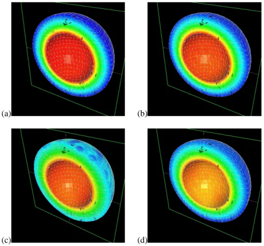
In figure-4, level set slices are shown for the fields u1 and u2 at convergence for noise

free and5% noisy data. The overall Nash algorithm (19) converged in 150 iterations. More

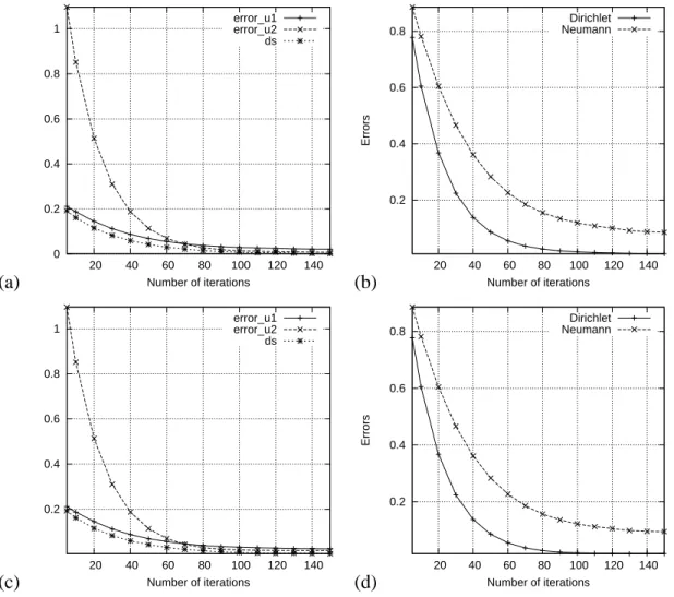
detailed issues related to the convergence are presented in figure-5. Relative L2-errors behave well in the noise free and in the noisy cases. The relative errors on reconstructed fields decrease as well as do the ones relative to the missing data (converged Nash strategies, which we recall are respectively the trace of u1and the normal trace of u2 over the sphereΓi).

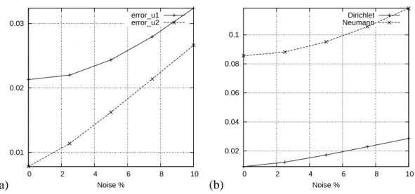
The sensitivity of the reconstructed fields and missing data to the noise level σ is shown in figure-6. Interestingly, boundary missing data are much less sensitive than the domain distributed fields. Both of them exhibit a satisfactory stable behavior w.r.t. the noise magnitude.

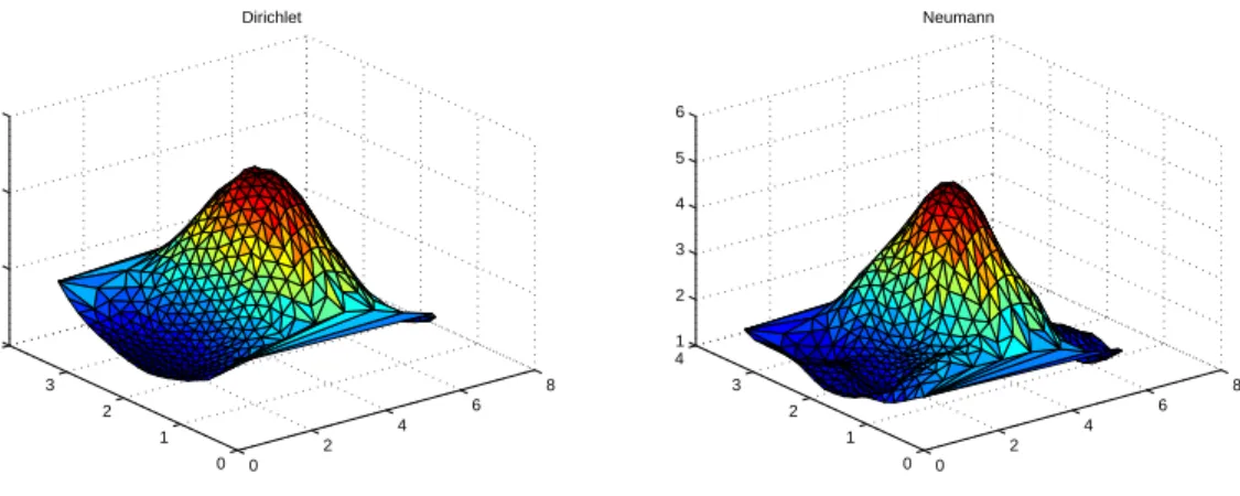
Test-case D. The second function is given by

u(x, y, z) = 1

p(x + 0.2)2_{+ y}2_{+ z}2. (26)

The function u given by (26) is the non-radial solution of ∆u = δX0, where the source term is now X0 = (−0.2, 0, 0).

In this experiment we put 5% of noise in (f, Φ) according to (23). The obtained

results are illustrated in figure-7, where the reconstructed fields u1 and u2 are presented at

convergence. The non radial missing data are presented in figure-8 and relative L2-errors on the reconstructed fields and boundary data are shown in figure-9.

Even though the error curves do monotonically decrease towards zero for the two test-cases C and D, the stagnation that appears quite early (around iterations 80-120 in the present case) suggests that multilevel or hierarchical optimization approaches should be designed to speed-up the convergence of the Nash algorithm.

6. Conclusion

Let us conclude the paper with some short remarks. First of all, we have used the

simplest class of games to model the completion problem, namely the class of static games with complete information. This simple game formulation yields interesting results like the existence and uniqueness of a Nash equilibrium even when the Cauchy data are not compatible, and also the fact that the Nash equilibrium is the missing data when the Cauchy

problem has a solution. Investigation of more sophisticated classes of games such as dynamical games with incomplete information may lead to new efficient data completion algorithms. It is also interesting to notice that solving the data completion problem with our method makes use of the standard computational tools, be it finite element or optimization codes. The numerical experiments presented for different test-cases prove that our method exhibits remarkable numerical stability with respect to noisy Cauchy data.

References

[1] Aboula¨ıch R, Ben Abda A and Kallel M 2008 Missing boundary data reconstruction via an approximate optimal control Inverse Problems and Imaging 2 411–426

[2] Alessandrini G, Rondi L, Rosset E and Vessella S 2009 The stability for the Cauchy problem for elliptic equations Inverse Problems 25 123004 (47pp)

[3] Andrieux S, Baranger T and Ben Abda A 2006 Solving Cauchy problems by minimizing an energy-like functional Inverse Problems 22 115–133

[4] Attouch H, Redont P and Soubeyran A 2007 A new class of alternating proximal minization algorithms with costs-to-move SIAM J. Optim. 18 1061–1081

[5] Attouch H, Bolte J, Redont P and Soubeyran A 2008 Alternating proximal algorithms for weakly coupled convex minimization problems. Applications to dynamical games and PDE’s J. Convex Anal. 15 485– 506

[6] Attouch H and Soueycatt M 2009 Augmented Lagrangian and proximal alternating direction methods of multipliers in Hilbert spaces. Applications to games, PDE’s and control Pacific J. Optim 5 17–37 [7] Basar T 1987 Relaxation techniques and asynchronous algorithms for on-line computation of

non-cooperative equilibria Journal of Economic Dynamics and Control 11 531–549

[8] Ben Abda A, Kallel M, Leblond J and Marmorat J-P 2002 Line-segment cracks recovery from incomplete boundary data Inverse Problems 18 1057–1077

[9] Ben Abda A, Ben Hassen F, Leblond J and Mahjoub M 2009 Sources recovery from boundary data: a model related to electroencephalography, Mathematical and Computer Modelling 49 2213–2223 [10] Ben Belgacem F 2007 Why is the Cauchy problem severely ill-posed? Inverse Problems 23 823–36 [11] Bourgeois L 2010 About stability and regularization of ill-posed elliptic Cauchy problems: the case ofC1,1

domains ESAIM: M2AN 44 715–35

[12] Chaabane S, Jaoua M and Leblond J 2003 Parameter identification for Laplace equation and approximation in analytic classes J. Inv. Ill-Posed Problems 11 35-57

[13] Cao H and Pereverzv S V 2007 The balancing principle for the regularization of elliptic Cauchy problems

Inverse Problems 23 1943–1961

[14] Chakib A and Nachaoui A 2006 Convergence analysis for finite element approximation to an inverse Cauchy problem Inverse Problems 22 1191–1206

[15] Cimeti`ere A, Delvare F, Jaoua M and Pons F 2001 Solution of the Cauchy problem using iterated Tikhonov regularization Inverse Problems 17 553–570

[16] Cimeti`ere A, Delvare F, Jaoua M, Kallel M and Pons F 2002 Recovery of cracks from incomplete boundary data Inverse Problems in Engineering 10 377–392

[17] Dinh Nho Hao and Lesnic D 2000 The Cauchy problem for Laplace’s equation via the conjugate gradient method IMA Journal of Applied Mathematics 65 199–217

[18] Habbal A 2005 A topology Nash game for tumoral antiangiogenesis Structural and Multidisciplinary

Optimization 30 404–412

[19] Habbal A, Petersson J and Thellner M 2004 Multidisciplinary topology optimization solved as a Nash game Int. J. Numer. Meth. Engng 61 949–963

[20] Hadamard J 1953 Lectures on Cauchy’s Problem in Linear Partial Differential Equation, Dover, New york USA

[21] Hecht F, Le Hyaric A and Pironneau O Freefem++, Univ. Pierre et Marie Curie, Paris, software available at http://www.freefem.org/ff++/

[22] Kozlov V A, Maz’ya V G and Fomin A V 1991 An iterative method for solving the Cauchy problems for elliptic equations Comput. Math. Phys. 31 45–52

[23] Li S and Basar T 1987 Distributed algorithms for the computation of noncooperative equilibria Automatica 23 523–533

[24] Uryas’ev S and Rubinstein R Y 1994 On relaxation algorithms in computation of noncooperative equilibria

0.5 1 1.5 -3 -2 -1 0 1 2 3 temperature angle exact_sol noise=1% noise=3% noise=5% -1.5 -1 -0.5 0 0.5 -3 -2 -1 0 1 2 3 flux angle exact_sol noise=1% noise=3% noise=5%

Figure 1. Test-case A. Reconstructed smooth Dirichlet (τN, left) and Neumann (ηN, right) data overΓi. The profiles are presented at convergence and for various amounts of noise level

σ ∈ {1%, 3%, 5%}. The corresponding traces of the exact solution are also plotted. The Finite

Element computations are performed with1529 nodes and 2788 triangles.

0 2 4 6 8 10 -3 -2 -1 0 1 2 3 temperature angle exact_sol noise=1% noise=3% noise=5% 0 20 40 60 80 100 -3 -2 -1 0 1 2 3 flux angle exact_sol noise=1% noise=3% noise=5%

Figure 2. Test-case B. Reconstructed singular Dirichlet (τN, left) and Neumann (ηN, right) data overΓi. The profiles are presented at convergence and for various amounts of noise level

σ ∈ {1%, 3%, 5%}. The corresponding traces of the exact solution are also plotted. The Finite

0.5 1 1.5 2 2.5 -3 -2 -1 0 1 2 3 temperature angle D_data tr(u2) -0.5 0 0.5 1 1.5 2 2.5 -3 -2 -1 0 1 2 3 flux angle N_data d(u1)/dn

Figure 3. Test-case A. Regularization of noisy Cauchy data (noise level isσ = 5%). At

convergence : (left) the smoothed profileu2(τN)|Γc (− line) is compared to the random f

σ (+ dots) ; (right) the smoothed flux profile k∇ ˜u1.ν|Γc(− line) is compared to Φ

σ_{(+ dots).}

(a) (b)

(c) (d)

Figure 4. Test-case C. Top row : noise level is0%. At convergence, we plot a plane slice of

the level sets of (a)u1and (b)u2. Bottom row : noise level is5%. At convergence, are plotted the level sets of (c)u1and (d)u2. The Finite Element computations are performed with4740 nodes and22795 tetrahedral elements.

(a) 0 0.2 0.4 0.6 0.8 1 20 40 60 80 100 120 140 Number of iterations error_u1 error_u2 ds (b) 0.2 0.4 0.6 0.8 20 40 60 80 100 120 140 Errors Number of iterations Dirichlet Neumann (c) 0.2 0.4 0.6 0.8 1 20 40 60 80 100 120 140 Number of iterations error_u1 error_u2 ds (d) 0.2 0.4 0.6 0.8 20 40 60 80 100 120 140 Errors Number of iterations Dirichlet Neumann

Figure 5. Test-case C. Top row : RelativeL2_{-errors are presented as a function of overall} Nash iterationsk, for a noise level σ = 0%. (a) reconstructed fields : ku(k)i − uk/kuk, i = 1, 2 and Nash strategiesds = kS(k)_{− S}(k−1)_{k ; (b) missing Dirichlet data : kτ}(k)_{− u}

|Γik/ku|Γik

and Neumann datakη(k)₋∂u ∂ν |Γik/k

∂u

∂ν |Γik. Bottom row : The corresponding relative errors

(a) 0.01 0.02 0.03 0 2 4 6 8 10 Noise % error_u1 error_u2 (b) 0.02 0.04 0.06 0.08 0.1 0 2 4 6 8 10 Noise % Dirichlet Neumann

Figure 6. Test-case C. Sensitivity of the reconstructed fields to noisy Cauchy data(fσ_{, Φ}σ_).

L2_{-errors are presented as a function of the noise level σ : (a) reconstructed fields :}

kui− uk/kuk, i = 1, 2 ; (b) missing data : Dirichlet kτN − u|Γik/ku|Γik and Neumann

kηN −∂u_{∂ν |Γi}k/k∂u_{∂ν |Γi}k.

(a) (b)

Figure 7. Test-case D. Non radial case. Noise level is5%. The level sets of the reconstructed

fields (a)u1and (b)u2 are presented at convergence. The Finite Element computations are performed with4740 nodes and 22795 tetrahedral elements.

0 2 4 6 8 0 1 2 3 4 1 1.5 2 2.5 Dirichlet 0 2 4 6 8 0 1 2 3 4 1 2 3 4 5 6 Neumann

Figure 8. Test-case D. Reconstructed non radial Dirichlet (τN, left) and Neumann (ηN, right) data overΓi. The profiles are presented at convergence and for a noise levelσ = 5%.

(a) 0.2 0.4 0.6 0.8 1 40 80 120 160 200 Number of iterations error_u1 error_u2 ds (b) 0.2 0.4 0.6 0.8 40 80 120 160 200 Errors Number of iterations Dirichlet Neumann

Figure 9. Test-case D. Relative L2_{-errors are presented for the non radial case as a} function of the overall Nash iterations. Noise level is5%. (a) reconstructed fields error : ku(k)i − uk/kuk, i = 1, 2 and Nash strategies ds = kS(k)− S(k−1)k ; (b) missing Dirichlet data :kτ(k)_{− u}

|Γik/ku|Γik and Neumann data kη

(k)₋∂u ∂ν |Γik/k

∂u ∂ν |Γik.