Shirking, Monitoring, and Risk Aversion

HAL Id: halshs-00965532

https://halshs.archives-ouvertes.fr/halshs-00965532

Preprint submitted on 19 May 2014

HAL is a multi-disciplinary open access archive for the deposit and dissemination of sci-entific research documents, whether they are pub-lished or not. The documents may come from teaching and research institutions in France or

L’archive ouverte pluridisciplinaire HAL, est destinée au dépôt et à la diffusion de documents scientifiques de niveau recherche, publiés ou non, émanant des établissements d’enseignement et de recherche français ou étrangers, des laboratoires

Shirking, Monitoring, and Risk Aversion

Seeun Jung, Kenneth Houngbedji

To cite this version:

WORKING PAPER N° 2014

– 11

Shirking, Monitoring, and Risk Aversion

Seeun Jung Kenneth Houngbedji

JEL Codes: C91 ; D61 ; D81 ;D86

Keywords: Shirking; Monitoring; Risk under Uncertainty; Effort

P

-

S

E

48, BD JOURDAN – E.N.S. – 75014 PARIS

TÉL. : 33(0) 1 43 13 63 00 – FAX : 33 (0) 1 43 13 63 10

www.pse.ens.fr

Shirking, Monitoring, and Risk Aversion

∗

Seeun Jung

and Kenneth Houngbedji

May 18, 2014

Abstract

This paper studies the effect of risk aversion on effort under different monitoring schemes. It uses a theoretical model which relaxes the assumption of agents being risk neutral, and investigates changes of effort as monitoring varies. The predictions of the theoretical model are tested using an original experimental setting where the level of risk aversion is measured and monitoring rates vary exogenously. Our re-sults show that shirking decreases with risk aversion, being female, and monitoring. Moreover, monitoring is more effective to curtail shirking behaviors for subjects who are less risk averse, although the size of the impact is rather small.

JEL Classification: C91 ; D61 ; D81 ;D86

Keywords: Shirking; Monitoring; Risk under Uncertainty; Effort

∗_{This work was supported by the French National Research Agency, through the program}

Investisse-ments d’Avenir, ANR-10–LABX-93-01.

†_{Paris School of Economics, Science-Po Paris - seeun.jung@sciencespo.fr} ‡_{Paris School of Economics - kenneth.houngbedji@ens.fr}

1

Motivation

Firms often face the agency dilemma. While firms’ objective is to maximize their profits, employees would like to maximize their utilities. On the firms’ side, workers’ efforts are needed in order to increase productivity and also firms’ profits. However, effort is costly for workers. As workers would like to minimize their cost in order to achieve higher utility, they look for opportunistic behaviors which could lower their cost.1

These behaviors are not in the firms’ favor as they might negatively affect workers’ productivity which also lowers the firms’ profits. Therefore, employers try to avoid these behaviors with several tools such as monitoring. There have been debates on whether monitoring works as employers often believe. Two different stories explain the different directions of the impact of monitoring. The crowding-out theory in psychology literature suggests that monitoring may reduce overall intrinsic motivation and work effort. Deci (1971), Deci

(1975), and Deci and Ryan(1999) argued that when workers feel that they are not being trusted or controlled, they lose their motivation to work and the economic incentives such as monetary rewards or sanctions are not as efficient as planned.2

Hence, according to this story, monitoring would decrease workers’ efforts.

On the other hand, in the principal-agent problem, workers are rational cheaters, and therefore provide less than the optimal level of effort when the marginal benefit of doing so exceeds its cost. Therefore, in this case monitoring motivates the agents to raise their effort level in order to reduce the risk of a penalty if they get caught shirking (Alchian and Demsetz (1971), Calvo and Wellisz (1978), Fama and Jensen (1983), Laffont and Martimort (2002), and Prendergast (1999)). There are a number of studies (Rickman and Witt, 2007; Nagin et al., 2002; Kerkvliet and Sigmund, 1999; Bunn et al., 1992;

Becker, 1968) that investigate the rational cheater model and observe the variation of effort in response to monitoring. Nevertheless, an empirical validation of the rational

1_{Shirking behavior occurs when the workers put less efforts than they are supposed to put according}

to their contract with their employers.

2_{For example, paying for blood donation would reduce the willingness to donate (Drago and Perlman}

(1989), Frey and Oberholzer-Gee (1997), Kreps (1997), Gneezy and Rustichini (2000),Bohnet et al. (2000),Frey and Jegen(2000), andBnabou and Tirole(2003)).

cheater model is difficult to establish outside of an experimental setting. Cheating is indeed difficult to detect and employers already enforce a wide set of schemes to discour-age their employees from shirking. Nagin et al. (2002) have set an experimental design that circumvents the empirical challenges listed above and provide empirical evidence of the rational cheater model. They ran a field experiment in 16 sites of call centers, in order to see the relationship between monitoring and work motivation. The call center operators were followed for weeks with different monitoring rates. Via callbacks3

, the authors found that the employees are acting as rational cheaters and would shirk more as monitoring rate decreases. More precisely the number of ‘bad calls’ responds to the call-back rate. When the monitoring rate increases, the number of bad calls decreases. Yet, allowing workers’ heterogeneity in various dimensions, those who had ‘positive atti-tudes’ towards firms did not respond to lower monitoring, which could be partly explained by the crowding-out theory. More recently Dickinson and Villeval (2008) explained the complementarity between the crowding-out theory and the agent problem in a principal-agent experimental setting. Their findings are two-fold: (i) both principals and principal-agents respond to extrinsic incentives, (ii) intrinsic motivation is crowded out when monitoring is above a certain threshold. Jitsophon and Mori(2013) found that, in addition, controlling decreases workers motivation and lower their productivity, by setting an Origami-task experiment.

In this paper, we would like to follow the rational cheater model, but with a relaxation of risk neutrality of workers. Risk aversion may explain the heterogeneity observed by

Nagin et al. (2002) in addition to the crowding-out effect. Attitudes towards risk could explain various economic behaviors: job-sorting decisions (Pfeifer (2011); Bonin et al.

(2007);Ekelund et al.(2005)), and wages (Pissarides(1974);Murphy et al.(1987);Moore

(1995); Hartog et al. (2003); Pannenberg (2007)). Also it has been shown that often individual risk aversion is negatively correlated with productivity and the wage (Gneezy

3_{Callbacks would be monitoring in this setting. Callbacks could catch the ‘bad calls’ which the}

operators self-claimed to be successful but turned out not to be. Of course, callbacks are costly, it is impossible to call-back every call reclaimed to be positive. So 100% monitoring is not efficient. The penalty when they got caught for their shirking (cheating) behavior would be job dismissal.

et al. (2003); Grund and Sliwka (2006); Cornelissen et al. (2011); Dohmen and Falk

(2011)). Risk-averse workers are found to dislike the competitive and stressful work environment where the payment is higher. When there is monitoring, would they be more afraid of getting caught and take monitoring more harshly than others? Here is our interest. As full monitoring is not possible, under any monitoring schemes, uncertainty is likely to play a role, in which case we can identify different behaviors according to individual risk aversion.

The objective of this paper is, therefore, an attempt to provide a unified theory of the rational cheater model where the assumption that the agents are risk neutral is relaxed. More specifically, we investigate whether the impact of monitoring depends on individual risk aversion. To illustrate our point, we set up an experimental design where individual risk aversion is measured. As we build onNagin et al. (2002) and exogenously change the perceived monitoring rate and observe the variation in effort by the agents, we address some concerns regarding endogeneity.

Among others, the experiment is original in its design since we control for the perceived monitoring rate and observe the shirking behavior of individuals along with their level of risk aversion. Our results contribute to the literature by addressing the effectiveness of monitoring as a necessary condition for preventing risk-averse individuals from shirking. The remainder of the paper is organized as follows. The conceptual framework will be explained in Section 2. Section 3 will set up the experimental design and the rele-vant model along with the simulation results. Finally, we will discuss the results of the experiment in Section 4, then conclude in Section 5.

2

Conceptual Framework:

Shirking behavior with

Monitoring

Here, we present a simple conceptual framework about the effect of the monitoring rate on shirking behavior with risk preferences. We start with a risk-neutral agent. First, we

define ‘shirking’ as putting less effort than the desired level. A firm gives the agent a contract with the desired effort e∗ _{and the wage of W}

e∗. If the agent accepts that offer,

he/she can decide whether to provide the full desired effort e∗_{, or less effort which we}

call ‘shirking effort’ es. By definition, the desired effort is greater than the shirking effort

(e∗ _{> e}

s). Then, with this effort provision, the agent can have different outcomes. The

production function Y is increasing with effort e, and therefore, the outcome with the desired effort is always better than the outcome when a shirking behavior is engaged (Y (e∗_{) > Y (e}

s)). According to the agent’s outcome, the wage is set as a piece-rate

wage scheme (bY (e)). An agent can have two different strategies: (1) provide the full contractual effort (payment: bY (e∗_{)) or (2) shirk by providing the shirking effort and}

pretend to have supplied the full effort e∗ _{and thus ask for the payment of bY (e}∗_{). In the}

latter case, there is a chance of being caught if the company has a monitoring system. With a probability of being caught (monitoring rate) of m, the agent who decides to shirk will be only paid according to what he actually does (payment : bY (es)) which is smaller

than the payment with the full effort (payment: bY (e∗_)).4

F irm W orker M onitoring Wes,1−m = bY (e∗) − C(es) N otD_etect 1 − m Wes,m = bY (es) − C(es) Detect m Shirk e_{s, C(e} s) We∗ = bY (e∗) − C(e∗) Respect e∗, C(e ∗) (e∗_{, W} e∗))

Figure 1: Shirking Decision Making under Monitoring Rate m

Also, as providing effort is costly, we can set a cost function which is increasing with effort e. Therefore supplying full effort is more costly than shirking (C(e∗_{) > C(e}

s)).

With this setting, there are three wealth states with monitoring rate m (defining No-Detect rate P = 1 − m)

- Shirking, detected : Wes,m= bY (es) − C(es)

- Shirking, claim to provide e∗_{, not detected : W}

es,1−m = bY (e∗) − C(es)

- No shirking : We∗ = bY (e∗) − C(e∗)

And, therefore, Wes,m < We∗ < Wes,1−m.

Then, we can now derive the optimal monitoring rate where the agent switches her shirking behavior. Taking the risk-neutral agent first, as her utility function is linear in wealth, the monitoring rate where the agent switches from shirking to not shirking is:

m∗ ₌ C(e

∗_{) − C(e} s)

b[Y (e∗_{) − Y (es)]}

calculated from the indifference condition of expected utility between shirking and not shirking

U[We∗] = mU [W_es,m] + (1 − m)U [W_es,1−m]

We∗ = mW_es,m+ (1 − m)W_es,1−m

bY(e∗_{) − C(e}∗_{) = m(bY (e}

s) − C(es)) + (1 − m)(bY (e∗) − C(es))

Therefore the optimal No-Detect rate for the risk-neutral agent is:

P∗ _{= 1 − m}∗ _{= 1 −} C(e ∗_{) − C(e} s) b[Y (e∗) − Y (e_s)] = We∗− W_es,m b[Y (e∗) − Y (e_s)]

Figure 2 illustrates the risk-neutral agent’s utility function. At the optimal level of the no-detect rate (P∗ _{= 1−monitoring rate m), the agent switches her shirking behavior.}

The risk-neutral agent’s optimal strategy with respect to P is

- 0 ≤ P < P∗_{, m}∗ _{< m ≤ 1 : U [W}

e∗] > mU [W_es,m] + (1 − m)U [W_es,1−m] : Does not

shirk

- P = P∗_{, m= m}∗ _{: U [W}

e∗] = mU [W_es,m] + (1 − m)U [W_es,1−m] : Indifferent between

Shirking and Not Shirking

- P∗ _{< P ≤ 1, 0 ≤ m < m}∗ _{: U [W}

The shirking disincentives can be seen in the lower triangle of Figure 2, where the agent does not shirk, while the shirking incentives are in the upper triangle, where she always shirks.

We now introduce two different types of agent (risk averse and risk seeking) in addition to the risk-neutral agent. Figure 3 draws the utility functions for each agent: the risk-neutral agent has a linear utility function, the risk-averse agent has a concave utility function, and the risk-seeking agent has a convex utility function with respect to wealth. Given that we now know the optimal level of the no-detect rate P∗ _{= P (RN )}∗_{for the}

risk-neutral agent, we can graphically obtain the optimal no detect rate for the risk-seeking agent P (RS)∗ _{and the risk-averse agent P (RA)}∗_{. Due to the concavity (convexity) of}

the utility function for the risk-averse (seeking) agent, the optimal no-detect rate of switching from not shirking to shirking is higher (lower) than that of the risk-neutral agent. In other words, the risk-averse agent will shirk at a lower monitoring rate (higher no-detect rate) than the risk-neutral agent, whereas the risk-seeking agent will shirk at a higher monitoring rate than the risk-neutral agent. Therefore, the switching no-detect rate for each agent is 0 < P (RS)∗ _{< P(RN )}∗ _{< P(RA)}∗ _{< 1, and we can, hence, infer}

the relationship between the optimal no-detect rate P∗ _{(the monitoring rate m}∗_{) and the}

risk parameter r (the higher is r, the greater is risk aversion):

∂P∗

∂r >0 → ∂m∗

∂r <0

which means, as they become more risk averse, agents switch from shirking to not shirking at lower monitoring rates. Once the agent decides to shirk, she will then choose the optimal level of shirking which will maximize her utility. We will discuss this in more details in the next Section.

W(shirking, detected) _{W(full effort)} W(shirking, not detected) W(s,d) W(e) W(s,nd) Wealth R is k N e u tr a l A g e n t's U ti li ty Shirking Incentive Shirking Disincentive P* P=0 P=1 0 < P < P* P* < P < 1 No Shirking Shirking

Figure 2: Shirking vs Not Shirking? Risk-Neutral Agent

P=0 P(RN)* P=1 W(s,d) W(e) W(s,nd) P = 1 - monitoring rate (m) U ti li ty P* P=0 P=1 P*(RS) < P(RN)* P(RN)* < P*(RA) Risk Averse Risk Seeker Risk Neutral

3

Experiment

3.1

Setting

We carry out a controlled experiment in which the subjects cannot select themselves into one group or another with regard to their risk aversion. Subjects are randomly allocated to their group and undergo the tasks assigned to their group. Therefore, the parameter of risk aversion is exogenous to the monitoring rate.5

The experiment involves solving tasks in a limited time period. Each task consists in counting even numbers in a fifteen-digit code to calculate the sum and compare this to a given number k.6

When the sum is equal to the given number k, the participant reports ‘true’, and ‘false’ otherwise. As we put the alternative with which participants have to compare to the answer that they calculate close to the correct answer (i.e. using a normal distribution with small variance), participants can learn that the given alternatives can be around the correct answer from the training session, which will make participants tempted to click ‘yes’ with guessing (i.e. shirking). As we asked to add all even numbers presented in a 15 digit-code, we only gave the even numbers as the given alternative for each code.

Since these exercises require no particular skills, we believe that no participant is disadvantaged.7

The participants report the number of codes solved on a piece of paper and are paid according to their performance. Before the experiement, the instruction of the experiment were given to the participants. We asked them to imagine that they were working for a cryptography firm where the profit is upon the number of codes solved

5_{All experiments were computerized using the REGATE software designed by Zeilliger (2000) and}

the program was set up by Maxim Frolov from the Centre d’Economie de la Sorbonne of the University of Paris 1. These experiments were held in Laboratoire d’Economie Experimentale de Paris (L.E.E.P) of the Paris School of Economics.

6

The code is generated by simulating n repeated Bernoulli draws of even and odd numbers with a probability p of getting an even number. The level of difficulty depends on the parameter p used to generate the code. The smaller p, the easier the item as there will be less even numbers to count in a code. The random number k is a code generated following the normal distribution with the mean of the sum, for example

7

It is possible that students who experience difficulties at reading might be disadvantaged. We can control for that by asking the participants to report whether they have been diagnosed with eyes issues.

right, and the salary is based on the performance. Starting with a training session, we gave participants four sessions assigning different monitoring rates. Each session lasts for 5 minutes.

Training Task: Participants are asked to decipher codes correctly in 5 minutes, and then paid a flat rate of 5 euros. Nothing is reviewed.

Treatment Task 1: Participants are asked to decipher codes correctly in 5 minutes. They are also told that all answers will be checked and that participants will be paid according to the correct answers.

Treatment Task 2: Participants are asked to decipher codes correctly in 5 minutes. They are also told that they will play a lottery after the task. With 60% probability, all answers will be checked and they will be paid according to the correct answers. With 40% probability, nothing will be reviewed, and they will be paid according to the numbers of codes they say they solved regardless of whether they are correct or not.

Treatment Task 3: Participants are asked to decipher codes correctly in 5 minutes. They are also told that they will play a lottery after the task. With 20% probability, all answers will be checked and they will be paid according to the correct answers. With 80% probability, nothing will be reviewed, and they will be paid according to the numbers of codes they say they solved regardless of whether they are correct or not.

For the purpose of the study we sampled 263 volunteers who are paid 10 cents per code deciphered with the flat wage of 5 euros for showing up and taking the training task. Since we also want to control for heterogeneity in attitudes towards risk, the subjects took a test measuring individual risk aversion. In order to avoid learning bias and ordering effects, we randomized the order of tasks 1, 2, and 3 for each subject.

Figure 4: Example of Task Screen

3.2

Model: Shirking behavior with Monitoring

In this section, we derive a set of predictions given the setting of the experiment. Assume that the number x of codes successfully deciphered by a participant depends on the effort esupplied. She shirks whenever she considers a code deciphered by guessing. For instance she makes a guess with the probability p(< 1) whether the sum of even numbers in a fifteen-digit code corresponds to the given number. To simplify the model, we assume that if the participant puts in enough effort, she gets the answer right, as counting is a reasonable easy task. We therefore assume a linear relationship between the effort and the outcome. In our case, effort ei corresponds to the number of codes for which the

subject provided the full desired effort. On the other hand, we define si, as shirking

behavior; the number of codes which the subject answered by guessing. The subjects are offered a linear contract of the form wi = bxi. We assume that supplying effort to solve

the codes is costly: c(ei) = ciei. Therefore, we consider shirking as shirking on quality.

When an individual shirks, then the quality of work decreases (i.e. the correction rate of solving codes is lower).

We here have two possible states of wealth depending on the monitoring rate m, when the subject allocates effort and determines shirking behavior (ei and si).

- shirking is detected with probability m, and the subject receives a wage according to the real outcome: b(ei+ psi) with cost c(ei). This utility is U [b(ei+ psi)] − c(ei)

- shirking is not detected with probability 1 − m, and the subject receives the full wage: b(ei+ si) with cost c(ei). This utility is U [b(ei+ si)] − c(ei)

The agent chooses the level of effort and shirking by maximizing her expected utility.

maxei,siEU[ei, si]

max m[U {b(ei+ psi)} − c(ei)] + (1 − m)[U {b(ei+ si)} − c(ei)]

s.t T ≥ veiei+ vsisi

T is the total time endowment that the subject can use in one task, and vei and vsi are the

time needed to provide effort and shirking, respectively. Using the negative exponential utility function with risk-aversion parameter ri (u(wi) = −exp[−riwi]), we can solve for

the optimal level of s∗

i via the first-order condition:

s∗ i =

ln(1 − m) − ln(m) + ln(c + ve− vs) − ln(vs− cp − vep)

rib(1 − p)

It is easy to see that optimal shirking is falls with the monitoring rate :

∂s∗ i ∂m = − 1 1−m − 1 m rib(1 − p) <0

However, when we look at the relationship between risk aversion and optimal shirking, it is more complex, and more conditions need to be applied in order to check the sign.

∂s∗ i ∂ri = −ln(1 − m) − ln(m) + ln(c + ve− vs) − ln(vs− cp − vep) r2 ib(1 − p) ∂s∗ i 2 ∂ri∂m = ( 1 1 − m + 1 m) 1 b(1 − p) 1 r2 i >0

−2

0

2

4

6

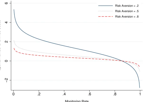
Optimal Number of Shirked Codes

0 .2 .4 .6 .8 1

Monitoring Rate

Risk Aversion = .2 Risk Aversion = .5 Risk Aversion = .8

Figure 5: Optimal Shirking with Monitoring

We, therefore, ran a simulation of our experiment environment. Figure 5 shows the simulation results for optimal shirking, which varies with the monitoring rate for different levels of risk aversion.8

This shows that optimal shirking decreases as the subject is more risk averse. Also as the monitoring rate rises, optimal shirking decreases. It also shows that at a lower level of monitoring rate, less risk-averse subjects are more sensitive to the monitoring rate increase, whereas the slopes of more risk-averse subjects are rather flat, and not much affected by the monitoring rate change. Indeed risk-averse agents tend to shirk less at any level of monitoring. After a certain high monitoring rate (85%), no one intends to shirk as optimal shirking falls below zero. We may infer that the full monitoring is not necessary under this setting. If enough monitoring is exerted, workers will not shirk. Figure 6 shows the shirking proportion by monitoring and risk aversion.

8

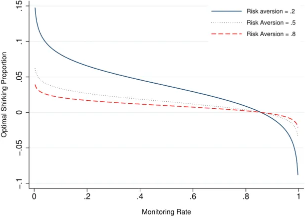
−.1 −.05 0 .05 .1 .15

Optimal Shirking Proportion

0 .2 .4 .6 .8 1

Monitoring Rate

Risk aversion = .2 Risk Aversion = .5 Risk Aversion = .8

Figure 6: Optimal Shirking Proportion with Monitoring The optimal shirking proportion is calculated as

e∗ i

e∗ i + s∗i

. When we compare less risk-averse agents to more risk-averse agents, both reduce their shirking proportion as monitoring increases. More risk-averse agents always have less incentives to shirk at any level of monitoring and have a rather flat slope, whereas less risk-averse agents shirk significantly more when monitoring is low enough. In this repre-sentation, the graph shows that the slope of the risk-averse agent is flatter than that of less risk-averse individuals, starting at the lower level of shirking proportion. We would thus like to test that (i) more risk-averse individuals shirk less (∂s∗

∂r <0), (ii) shirking falls

with monitoring (∂s∗

∂m <0), and (iii) more risk-averse individuals have a flatter shirking

slope with monitoring (∂2_s∗

∂r∂m >0). In order to test these three hypotheses, we set up an

4

Results

4.1

Data

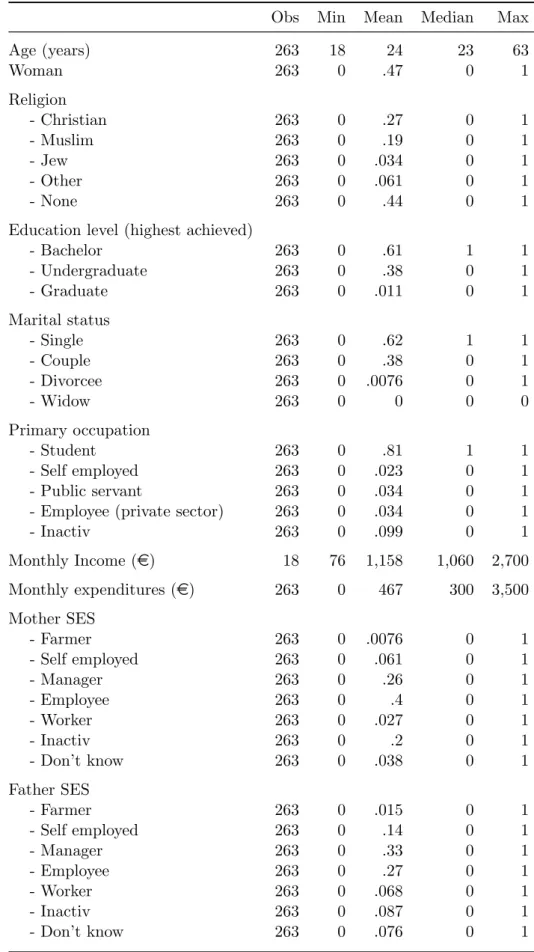
Table 1 presents the descriptive statistics of the samples we use for the experiment. Including the pilot session, we used 263 subjects. The average age is around 24, most of whom are students as the lab belongs to the University of Paris 1. About half of the subjects are female and religious. We also collected information on family background. Most of the subjects’ parents are employed or in managerial positions. In addition to socio-demographic information, we also gathered data on individual risk aversion.

Table 2gives the simple statistics for the risk-attitude questions. Subjects are asked to grade their risk attitudes on a 11-ladder Likert scale from 0 being extremely risk averse to 10 being extremely risk seeking. The average is around 5.2 which would be considered as risk neutral. The second methodology used to derive the individuals’ preferences towards risk elicits the individual’s willingness to pay for a lottery ticket. The level of risk aversion is measured via a series of questions, where each subject states her preference between 3 euros in cash and several fair lotteries of which the expected gains are 2, 2.5, 3, 3.5, 4, and 4.5 euros. On average, they would switch from cash to lottery when the expected gain is 3.5, which is higher than the certain cash amount. This suggests that subjects are somewhat risk averse at the mean. However the median is 3 euros, which is risk neutral. We also gathered various risk-related questions in order to create an aggregate measure of risk aversion `a la Arrondel and Masson(2010). We have questions on certainty equivalence, which measures the reservation price for the lottery. In these questions, the average reply is rather ‘risk averse’. We also asked for some behavior-related questions such as the average time of arrival before the scheduled departure at the train station or at the airport, as well as smoking and drinking. Using these questions, we created a score variable of risk aversion via the principal component analysis, with an increasing order (the higher, the more risk averse). We also simplify the self-reported measure into three outcomes of being risk seeking, risk neutral, and risk averse.

Table 1: Descriptive Statistics of Subjects.

Obs Min Mean Median Max

Age (years) 263 18 24 23 63 Woman 263 0 .47 0 1 Religion - Christian 263 0 .27 0 1 - Muslim 263 0 .19 0 1 - Jew 263 0 .034 0 1 - Other 263 0 .061 0 1 - None 263 0 .44 0 1

Education level (highest achieved)

- Bachelor 263 0 .61 1 1 - Undergraduate 263 0 .38 0 1 - Graduate 263 0 .011 0 1 Marital status - Single 263 0 .62 1 1 - Couple 263 0 .38 0 1 - Divorcee 263 0 .0076 0 1 - Widow 263 0 0 0 0 Primary occupation - Student 263 0 .81 1 1 - Self employed 263 0 .023 0 1 - Public servant 263 0 .034 0 1

- Employee (private sector) 263 0 .034 0 1

- Inactiv 263 0 .099 0 1

Monthly Income (e) 18 76 1,158 1,060 2,700

Monthly expenditures (e) 263 0 467 300 3,500

Mother SES - Farmer 263 0 .0076 0 1 - Self employed 263 0 .061 0 1 - Manager 263 0 .26 0 1 - Employee 263 0 .4 0 1 - Worker 263 0 .027 0 1 - Inactiv 263 0 .2 0 1 - Don’t know 263 0 .038 0 1 Father SES - Farmer 263 0 .015 0 1 - Self employed 263 0 .14 0 1 - Manager 263 0 .33 0 1 - Employee 263 0 .27 0 1 - Worker 263 0 .068 0 1 - Inactiv 263 0 .087 0 1 - Don’t know 263 0 .076 0 1

Table 2: Descriptive Statistics of Variables Related to Risk Aversion.

Obs Min Mean Median Max

Measures of risk aversion Self assessmenta

263 0 5.2 6 10

Lottery: Cash of 3e or lotteryb

263 0 3.5 3 6

Risk aversion scorec

263 -5.3 7.5e-10 .079 1.6

Certainty equivalent Maximum price for

- Lottery {1000e, 0.5, 0e}d

263 0 105 50 700

- Lottery {1000e, 0.2, 0e}e 263 0 30 10 500

Premium for the lottery {-1000e, 0.2, 0e}f

263 0 124 100 1,000

Attitudes towards risk

Take risk to escape boredom 263 0 .83 1 1

Lottery as opportunity to lose money 263 0 .37 0 1

Average time before scheduled departure

- Train (mins) 263 0 33 15 1,500

- Flight (mins) 263 0 107 90 1,800

The subject has used

- Drugs† 263 1 1 1 1

- Tobacco† 263 1 1.9 1 4

- Alcohol† 263 1 2.5 3 4

Other characteristics

Level of anxiety† 263 1 2.4 2 4

The subject cares about

- Food quality† 263 1 3.2 3 4

- Social norms and rules† 263 1 2.7 3 4

- Civism† 263 1 3.3 3 4

- Respect of road signs† 263 1 3.3 3 4

- Undergo tax evasion if risk-free† 263 1 2.5 2 4

†

Indicates that the variable is discrete and takes the values 1 ”No”, 2 ”Rather no”, 3 ”Sometimes” and 4 ”Yes”.

a

The subject self declares her or his level of risk aversion on a scale from 0 – extremely risk averse – to 10 – extremely risk seeker.

b

The level of risk aversion is measured via a series of questions where the subject states his preferences between 3e in cash and several fair lotteries of which the expected gains are 2, 2.5, 3, 3.5, 4 and 4.5e.

c

The level of risk aversion is measured as the principal component underlying the vari-ables self-reported risk aversion, lottery questions, price p50, price p20, time train and time flight.

d

The subject is asked to give the maximum price she or he is willing to pay for a lottery ticket which offers a best outcome of 1000e with a probability of 50% or a worse outcome of 0e.

e _{The subject is asked to give the maximum price she or he is willing to pay for a lottery}

ticket which offers a best outcome of 1000e with a probability of 20% or a worse outcome of 0e.

0 10 20 30 40 50 Frequency 0 1 2 3 4 5 6 7 8 9 10

Level of risk aversion (self assessment)

0 ≡ ”Extremely risk averse” → 5 ≡ ”Risk neutral” → 10 ≡ ”Extremely risk seeker”

Figure 7: Distribution of Self-Assessed Risk Aversion.

0 .1 .2 .3 .4 Frequency -6 -5 -4 -3 -2 -1 0 1 2

Risk aversion score (PCA)

-6 ≡ ”Extremely risk seeker” → 2 ≡ ”Extremely risk averse”

0 .2 .4 .6 .8 1 Density

Self assessment Cash or lottery

Least Risk Averse Medium Most Risk Averse

Figure 9: Level of Risk Aversion Across Methods

Figure 7 and Figure 8 show the distribution of our risk-aversion measures. Self-reported risk aversion is bell-shaped, whereas the aggregated measure is a little skewed as the scale is not balanced between risk seeking and risk aversion. Figure 9compares the self-reported and lottery measures. While the self-reported measure distributes subjects into three categories evenly, the lottery measure groups more subjects into the risk neutral regions.

Table 3 shows the correlation between the risk-aversion measures and related ques-tions. In this paper, we mainly focus on the aggregated measure (hereafter, RA PCA) and the self-reported measure (hereafter, RA Self). Both measures are significantly cor-related with each other and are consistently corcor-related with the other questions: more risk-averse subjects would pay less for the lottery tickets, show up earlier at the train station/airport, and smoke and drink less. Also risk-averse subjects are on average more anxious. When considering socio-demographic characteristics, women and the more re-ligious are more risk averse. At the end of the experiment, we asked subjects how they perceived the tasks they undertook: rather as a possibility of winning money or losing

money. Risk-averse subjects tend to perceive these tasks as losing money. This makes sense as risk-averse agents take the losing possibility more seriously.

Table 3: Pairwise Correlation Matrix. RA PCA RA Self RA Lottery RA PCA 1.0000 RA Self 0.4136* 1.0000 RA Lottery 0.3156* 0.2195* 1.0000 Price P50 -0.8010* -0.1863* -0.0880* Price P20 -0.7633* -0.1621* -0.0426 Insurance P20 -0.1243* 0.0905* -0.0088 Time Train 0.1288* 0.0499 -0.0065 Time Flight 0.1065* 0.1000* 0.0492 Tobacco -0.4447* 0.0057 -0.053 Alcohol -0.3903* -0.0506 -0.0949* Anxiety 0.1154* 0.1645* -0.0007 Woman 0.2932* 0.0983* -0.1135* Education 0.0181 0.1140* 0.1541* Religion 0.1255* -0.0047 -0.0561 Task 0.1681* 0.2072* 0.1603* a ⋆ _{5% significance.} b

Task : Did you consider the task as the possibility of win-ning money or losing money?

Figure 10 depicts the average time (in seconds) spent on each item. As the number of item reviewed increases, subjects tend to spend less time on each code. This might be due to the loss of concentration over time or rather a strategy to go over more codes as time becomes more pressing. In comparison to full monitoring (task1), subjects take less time for each code when there is only 20% of monitoring of their work (task3). Figure 11 shows the graph for the number of subjects on each item. It is clear that with 20% monitoring, more people reach higher item numbers, compared to when there is more intensive monitoring.

Table 4 shows the descriptive statistics of the variables measuring the subjects’ per-formance. In each task, we have information on the number of items reviewed by the subjects. On average, subjects solved 29 items per task. If the time spent is less than 5

0

5

10

15

20

Average time (secs)

1 6 11 16 21 26 31 36 41 46 51 56 61 66 71

Item Id

Task 0 Task 1 Task 2 Task 3

Figure 10: Average Time Spent on each Item Across Tasks

0 50 100 150 200 250

Number of subjects who tried

to solve the item

1 6 11 16 21 26 31 36 41 46 51 56 61 66 71

Item Id

Task 0 Task 1 Task 2 Task 3

0 50 100 150 200 250

Number of subjects with

correct answers

1 6 11 16 21 26 31 36 41 46 51 56 61 66 71

Item Id

Task 0 Task 1 Task 2 Task 3

Table 4: Descriptive Statistics of Variables Measuring the Subjects’ Perfor-mance.

Obs Min Mean Median Max

Number of items reviewed 1,052 5 29 26 70

Number of items reviewed in less than 5s. 1,052 0 13 6 70

Time spent on an item (secs) 30,047 0 6.9 5.8 205

Item is correctly revieweda

30,047 0 .79 1 1

Item is reviewed in less than 5s (Shirking) 30,047 0 .44 0 1 Item’s difficulty (the correct answer) 30,047 4 74 30 29.9

Answer is Yes (=1) 30,047 0 1 0 0.4

Payment received at the end:

- Task (e) 789 .7 2.8 2.5 7

- Experiment (e) 263 7.5 14 13 24

a_{It is a dummy variable equal to ”1” if the item has been correctly answered by the subject}

and ”0” if not.

seconds, we assume that the code is deciphered by shirking9

. In the experimental design, we set 4 seconds to get the answer buttons to appear in order to let participants decide whether to shirk or make an effort to solve, depending on the difficulty of the code. We expect that when the code seems more difficult with higher numbers to calculate, the probability of getting right and the time spent would increase. Also this 4-second rule could prevent the temptation to click continuously, and decrease the incentives to shirk by peer effect (i.e. hearing that the neighbour clicks continuously/shirking). As we put the alternative with which participants have to compare to the answer that they calcu-late close to the correct answer (i.e. using a normal distribution with small variance), participants can learn that the given alternatives can be around the correct answer from the training session, which will make participants tempted to click ‘yes’ with guessing (i.e. shirking). If we look at the correlation coefficient between the shirking item and whether the answer is ‘Yes’, it is indeed positive and significant (ρ= 0.1151 significant at the 1% level) inTable 5. In other words, when participants shirk, they tend to put more ‘Yes’.

Table 6 is the correlation matrix of risk aversion and the monitoring rate with the

9_{This is a proxy for shirking behavior. When we do the calculation, it is hard to solve the code within}

Table 5: Pairwise Correlation Matrix Item Level.

RA PCA RA Self Difficulty Yes Shirked Answer is Yes -0.0234* 0.0215* -0.0124

Item is Shirked -0.0342* -0.0490* -0.0220* 0.1151*

Time Spent 0.0249* 0.0418* 0.0423* -0.1185* -0.7418*

a ⋆ _{1% significance.}

Table 6: Pairwise Correlation Matrix Task Level. RA PCA RA Self Monitoring No. Shirking Items -0.1545* -0.0980* -0.2341* No. Items -0.1757* -0.1396* -0.1871* No. Correct Items -0.1469* -0.1015* -0.0372 Correct Proportion 0.0902* 0.1140* 0.2682*

a ⋆ _{1% significance.}

performance outcomes at the task level. More risk-averse subjects have fewer items that we assume to be guessed by shirking and fewer items reviewed in each task. They have also fewer correct items. However, this is because the code is [Yes/No] questions, so if you shirk and make a guess, still there is a chance of p which is greater than zero of getting the right answer. So if the subjects shirk a lot, this increases the number of correct items. Nonetheless, more risk-averse subjects have a higher proportion of correct items. Monitoring works in the same way as risk aversion. As monitoring becomes more intensive, there is less shirking, and fewer items solved, but the correction rate would increase.

Table 7 shows the subjects’ performance across tasks. Monitoring rates in Tasks 1, 2, and 3 are 100%, 60%, and 20%, respectively. At the task level, the table shows that as the monitoring rate reduces the number of items reviewed and the number of shirked items rise. At the item level, as the monitoring rate decreases, (i) the subjects spend less time on each item, (ii) the success rate of each item decreases, and (iii) the items are more likely to be reviewed by guessing.

Table 8 is a simple calculation of the monetary incentive to make people shirk across tasks. We calculated the difference in the number of shirking codes, and the difference in

Table 7: Subjects’ Performance Across Tasks.

Task 0† Task 1 Task 2 Task 3 Task level

Number of items reviewed 19.21 29.00 31.25 34.78

(0.47) (0.66) (0.82) (0.81) Number of items correctly reviewed 16.98 24.16 24.33 24.84 (0.43) (0.46) (0.46) (0.47) Number of items reviewed in less than 5s 3.13 11.13 15.15 20.79 (0.39) (0.76) (1.05) (1.18)

Payment received (e) . 2.42 2.81 3.29

(.) (0.05) (0.08) (0.08)

Observations 263 263 263 263

Item level

Time spent on an item (secs) 10.91 7.33 6.16 4.99

(0.11) (0.06) (0.06) (0.06)

Item correctly reviewed 0.88 0.83 0.78 0.71

(0.00) (0.00) (0.00) (0.00)

Item reviewed in less than 5s 0.16 0.38 0.48 0.60

(0.01) (0.01) (0.01) (0.01)

Observations 5053 7627 8220 9147

Standard errors are reported in parentheses.

†

Task 0 is the practice session. Participants get paied 5 euros as fixed rate.

Table 8: Money Incentive for Shirk-ing. Mean Sd Obs Risk Seeking 0.056 0.274 159 Risk Neutral 0.073 0.136 189 Risk Averse 0.063 0.172 137 a

The mean of money incentive is calcu-lated as the change of number of shirk-ing codes over tasks divided by the change of the gains over tasks.

Table 9: Subjects’ Performance Across Tasks and Risk Aversion.

Risk Seeker Risk Neutral Risk Averse

Task 0† Task 1 Task 2 Task 3 Task 0 Task 1 Task 2 Task 3 Task 0 Task 1 Task 2 Task 3 Panel A: Item Level

Time spent on an item (secs) 10.21 7.06 5.29 4.98 11.05 7.47 6.70 4.97 11.58 7.48 6.64 5.02 (0.21) (0.11) (0.11) (0.10) (0.14) (0.10) (0.10) (0.09) (0.25) (0.13) (0.13) (0.12)

Item correctly reviewed 0.86 0.80 0.72 0.71 0.90 0.85 0.82 0.72 0.89 0.86 0.80 0.71

(0.01) (0.01) (0.01) (0.01) (0.01) (0.01) (0.01) (0.01) (0.01) (0.01) (0.01) (0.01) Item reviewed in less than 5s 0.25 0.42 0.57 0.61 0.12 0.36 0.42 0.58 0.13 0.37 0.45 0.61 (0.01) (0.01) (0.01) (0.01) (0.01) (0.01) (0.01) (0.01) (0.01) (0.01) (0.01) (0.01)

Observations 1705 2752 3067 3228 1965 2874 3032 3503 1383 2001 2121 2416

Panel B: Task Level

Number of items reviewed 19.38 31.27 34.85 36.68 19.26 28.18 29.73 34.34 18.95 27.41 29.05 33.10 (1.04) (1.40) (1.73) (1.57) (0.61) (0.95) (1.08) (1.19) (0.74) (0.94) (1.32) (1.49) Number of items correctly reviewed 16.63 24.86 25.15 26.05 17.33 24.03 24.42 24.76 16.93 23.51 23.21 23.51 (0.93) (0.96) (0.94) (1.04) (0.58) (0.66) (0.64) (0.61) (0.75) (0.71) (0.79) (0.76) Number of items reviewed in less than 5s 4.80 13.16 20.00 22.33 2.22 10.11 12.51 19.88 2.41 10.12 12.99 20.19 (1.00) (1.52) (2.16) (2.08) (0.37) (1.12) (1.38) (1.88) (0.50) (1.25) (1.78) (2.27)

Payment received (e) . 2.48 3.10 3.48 . 2.40 2.70 3.32 . 2.35 2.62 3.01

(.) (0.10) (0.18) (0.15) (.) (0.07) (0.10) (0.12) (.) (0.07) (0.12) (0.14)

Observations 88 88 88 88 102 102 102 102 73 73 73 73

Standard errors are reported in parentheses. †

Task 0 is the training session. Participants get paid a fixed amount of 5 euros.

gains across tasks. On average, each shirking behavior would be induced by a monetary incentive of 6 cents. Risk seekers would shirk at a lower level of the monetary incentive than would others. Table 9 provides more detail on how the three different types (risk-seeking, risk-neutral, and risk-averse agents) change their performance across tasks. At both the task and item levels, we can observe that as subjects become more risk averse, and as monitoring increases, subjects review fewer items at each task, spend more time on solving codes, and therefore we find fewer shirked codes.

4.2

Analyses

We first start with the baseline analysis under full monitoring10

. RA PCA measures the level of risk aversion by aggregating various dimensions related to risk. It captures the core risk attitudes and reduces measurement errors and noise (Arrondel and Masson

(2010, 2011)).

Table 10shows the simple OLS results with clustered standard errors at the individual level. Risk aversion is negatively correlated with the number of shirking codes, the number of items reviewed, the number of correct codes, and the gains at the task level (Columns (1), (2), (3), and (5), respectively). Being risk averse reduced the probability that the code is deciphered by shirking (Column (6)) and increases the time spent on each item. However those estimates are not statistically significant. One interesting feature is that women shirk less, and also review fewer items. This pattern is quite similar to being risk averse and actually women are more risk averse. The difficulty of each item is also controlled. When the level of difficulty increases, it is likely to increase the time to solve the item, and also the probability of getting the right answer decreases. We could disentangle the impact on the shirking outcome that purely comes from risk aversion and monitoring. We should be careful when we interpret the number of correct items and the proportion of correct items (Column (4) and (5)). As explained earlier, the number of correct items may increase with shirking, as the probability of getting the right answer

10

Table 10: Risk Aversion under Full Monitoring

Task Level Item Level

(1) (2) (3) (4) (5) (6) (7) (8)

N Shirking N Items N Correct % Correct Gains Shirking Time Correct

Risk Aversion -0.882 -1.022 -0.629 0.007 -0.063 -0.016 0.257 0.009 (0.90) (0.80) (0.53) (0.01) (0.05) (0.02) (0.24) (0.01) Woman ( = 1) -5.250*** -3.900** -3.966*** -0.027 -0.398*** -0.124** 1.460*** -0.029 (1.47) (1.32) (0.93) (0.02) (0.09) (0.04) (0.43) (0.02) Age 0.048 0.181 0.098 -0.001 0.010 -0.001 0.024 -0.002 (0.13) (0.13) (0.08) (0.00) (0.01) (0.00) (0.03) (0.00) Graduate Student -0.961 0.015 0.479 0.017 0.047 -0.030 -0.012 0.015 (1.49) (1.23) (0.83) (0.01) (0.08) (0.04) (0.43) (0.02) Item Difficulty -0.005*** 0.063*** -0.000 (0.00) (0.01) (0.00) Constant 13.820*** 26.520*** 23.038*** 0.869*** 2.309*** 0.660*** 4.369*** 0.874*** (3.24) (3.15) (2.06) (0.03) (0.21) (0.08) (0.84) (0.04) R squared 0.061 0.058 0.096 0.018 0.096 0.032 0.034 0.003 Observations 263 263 263 263 263 7525 7525 7525 a ⋆ _10%,⋆⋆ _{5%, and}⋆⋆⋆ _{1% significance.} b

Standard errors are clustered at the individual level.

when shirking is greater than zero. Therefore, the proportion of correct items does not really vary with risk aversion even though the latter is negatively correlated with the number of correct answers. This might explain why the risk-averse workers’ productivity is lower, but the quality of work is better as they are more careful and take more time to do the work. In our paper, we want to estimate ∂y

∂m, ∂y ∂ra, and ∂2 y ∂m∂ra, where y is various proxies for shirking behavior such as the number of shirking codes, the number of items reviewed, whether the code is shirked, and the time spent to solve each code. The following specification is estimated :

yit = β0+ βmmt+ β_rarai+ β_m,ramt× rai+ β_xxi+ ǫ_it

However, we might be concerned that the attitude towards risk is correlated with unob-servables such as calculation ability or cognitive skills for computer work.

E[mt× ǫit | xik] = 0 and E[rait× ǫit | xit] 6= 0

We will, hence, estimate the model with first a random effect and then a fixed effect.

Table 11is the random-effect specification at the task level, andTable 13is at the item level. Our dependent variables are the number of shirking codes, the number of items reviewed, the number of correct items, the proportion of correct items, and gains. In the first five columns in Table 11the results present the pure risk aversion effects on shirking behavior, while in the last five Columns, we have the results of the cross derivatives of risk aversion and the monitoring rate. With the interaction terms, we allow for different slopes for risk aversion. Being more risk averse reduces the shirking behavior (the number of items reviewed) but also lowers gains11

. As monitoring increases, the shirking behaviors diminish significantly. When we look at the interaction terms, the risk-averse individuals have a flatter downward curve with the monitoring rate, although the estimates are not significant (except for the gains). We only have a small sample size (789), so capturing

Table 11: Task Level, Random Effect.

(1) (2) (3) (4) (5) (6) (7) (8) (9) (10)

N Shirking N Items N Correct % Correct Gains N Shirking N Items N Correct % Correct Gains

Risk Aversion -1.448 -1.450* -0.589 0.012 -0.124* -2.049* -1.798* -0.563 0.019* -0.195**

(0.76) (0.66) (0.42) (0.01) (0.06) (1.00) (0.76) (0.46) (0.01) (0.07)

Monitoring Rate = 20% (ref)

Monitoring Rate = 60% -5.639*** -3.525*** -0.517 0.063*** -0.471*** -5.639*** -3.525*** -0.517 0.063*** -0.471*** (1.13) (0.68) (0.34) (0.01) (0.07) (1.13) (0.67) (0.34) (0.01) (0.07) Monitoring Rate = 100% -9.654*** -5.779*** -0.681* 0.099*** -0.870*** -9.654*** -5.779*** -0.681* 0.099*** -0.870*** (1.13) (0.68) (0.34) (0.01) (0.07) (1.13) (0.67) (0.34) (0.01) (0.07) RA x Monitoring 20% (ref) RA x Monitoring 60% 0.249 0.040 0.038 -0.003 0.069 (1.13) (0.68) (0.34) (0.01) (0.07) RA x Monitoring 100% 1.556 1.004 -0.117 -0.018 0.144* (1.13) (0.68) (0.34) (0.01) (0.07) Woman (=1) -7.879*** -5.429*** -3.606*** 0.011 -0.482*** -7.879*** -5.429*** -3.606*** 0.011 -0.482*** (1.52) (1.32) (0.84) (0.01) (0.11) (1.52) (1.32) (0.84) (0.01) (0.11) Age -0.081 0.093 0.053 -0.001 0.008 -0.081 0.093 0.053 -0.001 0.008 (0.14) (0.12) (0.08) (0.00) (0.01) (0.14) (0.12) (0.08) (0.00) (0.01) Graduate Student 1.023 1.162 1.028 0.008 0.148 1.023 1.162 1.028 0.008 0.148 (1.47) (1.28) (0.81) (0.01) (0.11) (1.47) (1.28) (0.81) (0.01) (0.11) Constant 25.001*** 33.501*** 23.857*** 0.751*** 3.116*** 25.001*** 33.501*** 23.857*** 0.751*** 3.116*** (3.49) (3.00) (1.90) (0.03) (0.26) (3.49) (3.00) (1.90) (0.03) (0.26) R squared Within 0.123 0.124 0.008 0.160 0.223 0.127 0.129 0.009 0.166 0.230 R squared Between 0.139 0.107 0.099 0.018 0.115 0.139 0.107 0.099 0.018 0.115 R squared Overall 0.132 0.112 0.083 0.084 0.158 0.133 0.113 0.083 0.086 0.161 Chi square 115.100 105.383 32.800 104.596 184.172 117.300 108.328 33.007 108.619 188.925 Observation 789 789 789 789 789 789 789 789 789 789 a ⋆_10%,⋆⋆_{5%, and}⋆⋆⋆_{1% significance.} 29

Table 12: Task Level, Fixed Effect.

(1) (2) (3) (4) (5)

N Shirking N Items N Correct % Correct Gains Monitoring Rate = 20% (ref)

Monitoring Rate = 60% -5.639*** -3.525*** -0.517 0.063*** -0.471*** (1.13) (0.67) (0.34) (0.01) (0.07) Monitoring Rate = 100% -9.654*** -5.779*** -0.681* 0.099*** -0.870*** (1.13) (0.67) (0.34) (0.01) (0.07) RA x Monitoring 20% (ref) RA x Monitoring 60% 0.249 0.040 0.038 -0.003 0.069 (1.13) (0.68) (0.34) (0.01) (0.07) RA x Monitoring 100% 1.556 1.004 -0.117 -0.018 0.144* (1.13) (0.68) (0.34) (0.01) (0.07) Constant 20.787*** 34.779*** 24.844*** 0.755*** 3.285*** (0.80) (0.48) (0.24) (0.01) (0.05) R-squared 0.127 0.129 0.009 0.166 0.230 Observations 789 789 789 789 789 a ⋆ _10%,⋆⋆_{5%, and}⋆⋆⋆ _{1% significance.}

Table 13: Item Level, Random Effect.

(1) (2) (3) (4) (5) (6)

Shirking Time Correct Shirking Time Correct

Risk Aversion -0.022 0.510** 0.014* -0.027* 0.537** 0.018*

(0.01) (0.18) (0.01) (0.01) (0.19) (0.01) Monitoring Rate = 20% (ref)

Monitoring Rate = 60% -0.111*** 1.125*** 0.066*** -0.110*** 1.131*** 0.066*** (0.01) (0.07) (0.01) (0.01) (0.07) (0.01) Monitoring Rate = 100% -0.201*** 2.173*** 0.111*** -0.200*** 2.162*** 0.110*** (0.01) (0.07) (0.01) (0.01) (0.07) (0.01) RA x Monitoring 20% (ref) RA x Monitoring 60% 0.003 0.096 0.003 (0.01) (0.07) (0.01) RA x Monitoring 100% 0.015* -0.193** -0.017** (0.01) (0.07) (0.01) Woman ( = 1) -0.160*** 1.930*** 0.017 -0.160*** 1.930*** 0.017 (0.02) (0.37) (0.01) (0.02) (0.37) (0.01) Age -0.003 0.023 -0.001 -0.003 0.023 -0.001 (0.00) (0.03) (0.00) (0.00) (0.03) (0.00) Graduate Student 0.024 -0.586 0.009 0.024 -0.584 0.009 (0.02) (0.35) (0.01) (0.02) (0.35) (0.01) Item Difficulty -0.002*** 0.031*** -0.002*** -0.002*** 0.031*** -0.002*** (0.00) (0.00) (0.00) (0.00) (0.00) (0.00) Constant 0.695*** 4.500*** 0.793*** 0.695*** 4.494*** 0.792*** (0.05) (0.83) (0.03) (0.05) (0.83) (0.03) R squared Within 0.038 0.040 0.016 0.038 0.041 0.017 R squared Between 0.153 0.120 0.067 0.152 0.120 0.069 R squared Overall 0.067 0.071 0.020 0.068 0.071 0.020 Chi square 1030.952 1072.991 418.368 1036.420 1089.344 430.091 Observations 24994 24994 24994 24994 24994 24994 a ⋆_10%,⋆⋆_{5%, and}⋆⋆⋆_{1% significance.}

Table 14: Item Level, Fixed Effect.

(1) (2) (3) (4) (5) (6)

Shirking Time Correct Shirking Time Correct Monitoring Rate = 20% (ref)

Monitoring Rate = 60% -0.110*** 1.120*** 0.065*** -0.110*** 1.126*** 0.065*** (0.01) (0.07) (0.01) (0.01) (0.07) (0.01) Monitoring Rate = 100% -0.200*** 2.168*** 0.110*** -0.199*** 2.157*** 0.109*** (0.01) (0.07) (0.01) (0.01) (0.07) (0.01) RA x Monitoring 20% (ref) RA x Monitoring 60% 0.003 0.095 0.002 (0.01) (0.07) (0.01) RA x Monitoring 100% 0.015* -0.194** -0.017** (0.01) (0.07) (0.01) Item Difficulty -0.002*** 0.031*** -0.002*** -0.002*** 0.031*** -0.002*** (0.00) (0.00) (0.00) (0.00) (0.00) (0.00) Constant 0.636*** 4.239*** 0.778*** 0.636*** 4.237*** 0.778*** (0.01) (0.09) (0.01) (0.01) (0.09) (0.01) R-squared 0.038 0.040 0.016 0.038 0.041 0.017 Observations 24491 24491 24491 24491 24491 24491 a ⋆_10%,⋆⋆_{5%, and}⋆⋆⋆_{1% significance.}

any small marginal change due to risk aversion might be difficult. At the item level, the estimates become more significant as we now have more observations. Allowing subject ability to vary at each task (random effect), we observe that risk-averse subjects spend more time on each item, and succeed in finding the correct answer. However, again, with interactions, it reduces the size of marginal effects (the slopes are flatter) as the interactions have opposite signs. Risk-averse subjects shirk less from the beginning (20% monitoring rate) and do not respond so much as less risk-averse subjects who shirk more and then modify their behaviors more as the monitoring rate changes, which is what we expected from our theoretical framework and simulation results. More strictly we run a fixed-effect model. The fixed effect can control for unobservables which might be correlated with individual risk-aversion and ability, and correct for the omitted variable bias. However, in the fixed effect specification, we can only observe the marginal effect of monitoring changes and the interaction terms, as individual risk aversion level is absorbed into the individual fixed effect. Table 12 gives the results at the task level. Similar to the random-effect model, greater monitoring reduces shirking. Also we have different signs for the interaction terms, meaning that the risk-averse individuals respond less to monitoring. Table 14 shows more significant coefficients with a larger sample size.

Intensive monitoring reduces shirking, but less for risk-averse subjects.

Overall, with our specification, we can observe that (i) risk-averse subjects shirk less, (ii) intensive monitoring reduces shirking, and (iii) risk-averse subjects respond less to the monitoring rate.12

However, the second degree of the impact of risk aversion for monitoring (cross derivative of risk averion and monitoring) is rather marginal, while gender and monitoring play important roles.

5

Concluding Remarks

This paper has investigated shirking with risk aversion under different monitoring schemes. A conceptual model explains that risk-averse subjects switch from shirking to not shirking at a lower monitoring rate in comparison to less risk-averse subjects. In our setting, sub-jects decide whether to shirk or put in an effort in order to solve given codes across tasks with different monitoring rates. We derive a relevant theoretical model and the simula-tion results show that risk aversion is negatively correlated with shirking in general, and so is the monitoring rate. When more intensive monitoring is exerted, individuals shirk less, but the size of any change differs by risk aversion. As more risk-averse agents shirk less at any level of monitoring, they respond less to the monitoring change in comparison to less risk-averse agents.

The experiment contains a series of codes to decipher. The objective of the task is to solve as many codes as possible under different payment schemes. With an uncertain probability, subjects can be paid either only for correct answers or with more luck for the number of items they tried to solve regardless of whether they are correct or not. This corresponds to a real work environment where the firm cannot really monitor every piece produced by the employees. In this setting, we observe that indeed risk-averse subjects behave differently than risk-seekers: they shirk less under uncertainty. Also

12

We observe similar results when we analyze shirking behaviors between genders. As women are more risk averse in general, we consider women as representative of risk-averse individuals. The results are presented at the task level in Table 15 and at the item level in Table 16. Women’s behavior is very similar to risk-averse individuals: they shirk less and respond less to changes in the monitoring rate.

monitoring works as we expected from the rational cheater model: it reduces shirking behavior. Looking at the slope of the impact of monitoring on shirking, that of risk-averse subjects is flatter than that of less risk-averse subjects, as expected from the theoretical framework; less risk-averse subjects shirk more at lower monitoring rates and they modify their behaviors sharply as monitoring increases.

We, therefore, validate the effectiveness of monitoring as a necessary condition for preventing shirking. In addition, we suggest that risk-averse agents may earn less under a piece-rate contract due to their lower productivity. As they do not bet on the outcome of not getting caught when shirking, but provide more effort to avoid mistakes, they produce less. However the quality of their work is better. That leaves an open question of whether firms should search for greater productivity or better work quality. This subject is useful on further research which remains to be carried out on the firms’ side.

References

Abdellaoui, M., A. Driouchi, and O. L’Haridon (2011). Risk aversion elicitation: recon-ciling tractability and bias minimization. Theory and Decision 71, 63–80.

Abeler, J., A. Falk, L. Goette, and D. Huffman (2009, January). Reference points and effort provision. IZA Discussion Papers 3939, Institute for the Study of Labor (IZA).

Alchian, A. A. and H. Demsetz (1971, May). Production, information costs and eco-nomic organizations. UCLA Ecoeco-nomics Working Papers 10A, UCLA Department of Economics.

Arrondel, L. and A. Masson (2010, June). French savers in the economic crisis : What has changed ? variation of preferences or simple adaptation to a new environment. mimeo, Paris-Jourdan Sciences Economiques.

Arrondel, L. and A. Masson (2011). La crise a-t-elle rendu l’pargnant plus prudent ? Retraite et socit 60 (1), 111–135.

Basov, S. and X. Yin (2010). Optimal screening by risk-averse principals. The B.E. Journal of Theoretical Economics 10 (1), 8.

Becker, G. S. (1968). Crime and punishment: An economic approach. Journal of Political Economy 76, 169.

Bohnet, I., B. S. Frey, and S. Huck (2000). More order with less law: On contract enforcement, trust, and crowding. Institute for Empirical Research in Economics -University of Zurich, Working Paper 52 (052).

Bonin, H., T. Dohmen, A. Falk, D. Huffman, and U. Sunde (2007, December). Cross-sectional earnings risk and occupational sorting: The role of risk attitudes. Labour Economics 14 (6), 926–937.

Bruggen, A. and M. Strobel (2007, August). Real effort versus chosen effort in experi-ments. Economics Letters 96 (2), 232–236.

Bunn, D. N., S. B. Caudill, and D. M. Gropper (1992). Crime in the classroom: An eco-nomic analysis of undergraduate student cheating behavior. The Journal of Ecoeco-nomic Education 23 (3), pp. 197–207.

Bnabou, R. and J. Tirole (2003). Intrinsic and extrinsic motivation. Review of Economic Studies 70 (3), 489–520.

Cadsby, C. B., F. Song, and F. Tapon (2010). Are you paying your employees to cheat? an experimental investigation. The B.E. Journal of Economic Analysis & Policy 10 (1), 35.

Calvo, G. A. and S. Wellisz (1978, October). Supervision, loss of control, and the optimum size of the firm. Journal of Political Economy 86 (5), 943–52.

Chouikhi, O. and S. V. Ramani (2004, 03). Risk aversion and the efficiency wage contract. LABOUR 18 (1), 53–73.

Clementi, F. (2011, March). The role of the experiment in the evolution of labor leg-islation: A perspective on constitutional law. In The Role of Experiments for the Advancement of Effective Labour Legislation. SSRN.

Cornelissen, T., J. S. Heywood, and U. Jirjahn (2011, April). Performance pay, risk attitudes and job satisfaction. Labour Economics 18 (2), 229–239.

Deci, E. L. (1971). Effects of externally mediated rewards on intrinsic motivation. Journal of Personality and Social Psychology 18(1), 105–115.

Deci, E. L. (1975). Intrinsic Motivation. New-York: Plenum Press.

Deci, Edward L.; Koestner, R. and R. M. Ryan (1999). A meta-analytic review of exper-iments examining the effects of extrinsic rewards on intrinsic motivation. Psychological Bulletin 125(3), 627–68.

Dickinson, D. and M.-C. Villeval (2008). Does monitoring decrease work effort? the complementarity between agency and crowding-out theories. Games and Economic Behavrior 63 (1), 56–76.

Dohmen, T. and A. Falk (2011, April). Performance pay and multidimensional sorting: Productivity, preferences, and gender. American Economic Review 101 (2), 556–90.

Dohmen, T., A. Falk, D. Huffman, U. Sunde, J. Schupp, and G. Wagner (2009). Individual risk attitudes: Measurement, determinants and behavioral consequences. Research Memoranda 007, Maastricht : ROA, Research Centre for Education and the Labour Market.

Drago, R. and R. Perlman (1989). Microeconomic Issues in Labour Economics: New Approaches., Chapter Supervision and High Wages as Competing Incentives: A Basis for Labour Segmentation Theory, pp. 41–61. New-York: Harvester Wheatsheaf.

Ekelund, J., E. Johansson, M.-R. Jarvelin, and D. Lichtermann (2005, October). Self-employment and risk aversion–evidence from psychological test data. Labour Eco-nomics 12 (5), 649–659.

Falk, A. and J. J. Heckman (2009, October). Lab experiments are a major source of knowledge in the social sciences. IZA Discussion Papers 4540, Institute for the Study of Labor (IZA).

Fama, E. F. and M. C. Jensen (1983, June). Separation of ownership and control. Journal of Law and Economics 26 (2), 301–25.

Fochmann, M., J. Weimann, K. Blaufus, J. Hundsdoerfer, and D. Kiesewetter (2010). Grosswage illusion in a real effort experiment. FEMM Working Papers 100009, Otto-von-Guericke University Magdeburg, Faculty of Economics and Management.

evi-dence. Institute for Empirical Research in Economics - University of Zurich, Working Paper 49 (049).

Frey, B. S. and F. Oberholzer-Gee (1997, September). The cost of price incentives: An empirical analysis of motivation crowding-out. American Economic Review 87 (4), 746–55.

Gneezy, U. and J. A. List (2006, 09). Putting behavioral economics to work: Testing for gift exchange in labor markets using field experiments. Econometrica 74 (5), 1365–1384.

Gneezy, U., M. Niederle, and A. Rustichini (2003, August). Performance in competitive environments: Gender differences. The Quarterly Journal of Economics 118 (3), 1049– 1074.

Gneezy, U. and A. Rustichini (2000, January). A fine is a price. The Journal of Legal Studies 29 (1), 1–17.

Golan, L., C. Parlour, and U. Rajan (2007, November). Racing to the bottom: Competi-tion and quality. GSIA Working Papers 2008-E33, Carnegie Mellon University, Tepper School of Business.

Goldstone, R. L. and C. Chin (1993). Dishonesty in Self-Report of copies made - moral relativity and the copy machine. Basic and Applied Social Psychology 14 (1), 19–32.

Grund, C. and D. Sliwka (2006, March). Performance pay and risk aversion. Discussion Papers 101, SFB/TR 15 Governance and the Efficiency of Economic Systems, Free University of Berlin, Humboldt University of Berlin, University of Bonn, University of Mannheim, University of Munich.

Hartog, J., E. Plug, L. Diaz-Serrano, and J. Vieira (2003, July). Risk compensation in wages - a replication. Empirical Economics 28 (3), 639–647.

Holmstrom, B. (1979, Spring). Moral hazard and observability. Bell Journal of Eco-nomics 10 (1), 74–91.

Jitsophon, S. and T. Mori (2013). The hidden costs of control in the field. Working Paper, Osaka University.

Kerkvliet, J. and C. L. Sigmund (1999). Can we control cheating in the classroom? Journal of Economic Education 30 (4), 331–343.

Kreps, D. M. (1997, May). Intrinsic motivation and extrinsic incentives. American Economic Review 87 (2), 359–64.

Laffont, J.-J. and D. Martimort (2002). The Theory of Incentives: The Principal-Agent Model. Princeton: Princeton University Press.

Mazar, N., O. Amir, and D. Ariely (2008, November). The dishonesty of honest people: A theory of self-concept maintenance. Journal of Marketing Research 45 (6), 633–644.

Moore, M. J. (1995, January). Unions, employment risks, and market provision of em-ployment risk differentials. Journal of Risk and Uncertainty 10 (1), 57–70.

Murphy, K. M., R. H. Topel, K. Lang, and J. S. Leonard (1987). Unemployment, risk, and earnings: Testing for equalizing wage differences in the labor market. In K. Lang and J. S. Leonard (Eds.), Unemployment and the Structure of Labor Markets, pp. 103–140. New York: Basil Blackwell.

Nagin, D. S., J. B. Rebitzer, S. Sanders, and L. J. Taylor (2002). Monitoring, motivation, and management: The determinants of opportunistic behavior in a field experiment. American Economic Review 92 (4), 850–873.

Pannenberg, M. (2007). Risk aversion and reservation wages. IZA Discussion Papers 2806, Institute for the Study of Labor (IZA).

Pfeifer, C. (2011). Risk aversion and sorting into public sector employment. Technical Report vol. 12(1), pages 85-99, 02, German Economic Review, Verein fr Socialpolitik.

Pissarides, C. A. (1974, Nov.-Dec.). Risk, job search, and income distribution. Journal of Political Economy 82 (6), 1255–67.

Prendergast, C. (1999, March). The provision of incentives in firms. Journal of Economic Literature 37 (1), 7–63.

Preston, J. and D. M. Wegner (2007). The eureka error: Inadvertent plagiarism by misattributions of effort. Journal of Personality and Social Psychology 92 (4), 575 – 584.

Rick, S., G. Loewenstein, J. R. Monterosso, D. D. Langleben, N. Mazar, O. Amir, and D. Ariely (2008, November). Commentaries and rejoinder to the dishonesty of honest people. Journal of Marketing Research 45 (6), 645–653.

Rickman, N. and R. Witt (2007). The determinants of employee crime in the uk. Eco-nomica 74 (293), 161–175.

Schwieren, C. and D. Weichselbaumer (2010, June). Does competition enhance perfor-mance or cheating? a laboratory experiment. Journal of Economic Psychology 31 (3), 241–253.

van Dijk, F., J. Sonnemans, and F. van Winden (2001, February). Incentive systems in a real effort experiment. European Economic Review 45 (2), 187–214.

Table 15: Gender Test: Task Level.

(1) (2) (3) (4) (5) (6) (7) (8) (9) (10)

N Shirking N Items N Correct % Correct Gains N Shirking N Items N Correct % Correct Gains Monitoring Rate = 20% (ref)

Monitoring Rate = 60% -8.568*** -5.252*** -0.619 0.093*** -0.630*** -8.568*** -5.252*** -0.619 0.093*** -0.630***

(1.54) (0.92) (0.47) (0.01) (0.10) (1.54) (0.92) (0.47) (0.01) (0.10)

Monitoring Rate = 100% -13.338*** -7.986*** -0.504 0.144*** -1.036*** -13.338*** -7.986*** -0.504 0.144*** -1.036***

(1.54) (0.92) (0.47) (0.01) (0.10) (1.54) (0.92) (0.47) (0.01) (0.10)

Woman (=1) x Monitoring 20% (ref)

Woman (=1) x Monitoring 60% 6.214** 3.663** 0.215 -0.063** 0.337* 6.214** 3.663** 0.215 -0.063** 0.337* (2.24) (1.34) (0.68) (0.02) (0.14) (2.24) (1.34) (0.68) (0.02) (0.14) Woman (=1) x Monitoring 100% 7.814*** 4.679*** -0.375 -0.094*** 0.353* 7.814*** 4.679*** -0.375 -0.094*** 0.353* (2.24) (1.34) (0.68) (0.02) (0.14) (2.24) (1.34) (0.68) (0.02) (0.14) Woman ( = 1) -13.407*** -9.063*** -3.900*** 0.070*** -0.785*** (1.95) (1.49) (0.90) (0.02) (0.14) Age -0.079 0.096 0.054 -0.001 0.008 (0.14) (0.12) (0.08) (0.00) (0.01) Graduate Student 0.957 1.097 1.001 0.009 0.142 (1.48) (1.28) (0.81) (0.01) (0.11) Constant 27.635*** 35.242*** 24.007*** 0.723*** 3.261*** 20.787*** 34.779*** 24.844*** 0.755*** 3.285*** (3.55) (3.04) (1.91) (0.03) (0.26) (0.79) (0.47) (0.24) (0.01) (0.05) Method RE RE RE RE RE FE FE FE FE FE R squared Within 0.145 0.147 0.010 0.196 0.235 0.145 0.147 0.010 0.196 0.235 R squared Between 0.127 0.090 0.092 0.008 0.098 0.125 0.084 0.083 0.006 0.087 R squared Overall 0.135 0.106 0.077 0.094 0.153 0.010 0.004 0.004 0.054 0.050 Chi square 126.228 115.304 31.472 129.437 188.632 Observations 789 789 789 789 789 789 789 789 789 789 a ⋆_10%,⋆⋆_{5%, and}⋆⋆⋆_{1% significance.} 40

Table 16: Gender Test: Item Level.

(1) (2) (3) (4) (5) (6)

Shirking Time Correct Shirking Time Correct Monitoring Rate = 20% (ref)

Monitoring Rate = 60% -0.154*** 1.611*** 0.094*** -0.153*** 1.607*** 0.094*** (0.01) (0.09) (0.01) (0.01) (0.09) (0.01) Monitoring Rate = 100% -0.247*** 2.748*** 0.152*** -0.246*** 2.743*** 0.150***

(0.01) (0.10) (0.01) (0.01) (0.10) (0.01) Woman (=1) x Monitoring 20% (ref)

Woman (=1) x Monitoring 60% 0.103*** -1.170*** -0.069*** 0.104*** -1.173*** -0.069*** (0.01) (0.15) (0.01) (0.01) (0.14) (0.01) Woman (=1) x Monitoring 100% 0.110*** -1.368*** -0.097*** 0.110*** -1.369*** -0.095*** (0.01) (0.15) (0.01) (0.01) (0.15) (0.01) Woman ( = 1) -0.241*** 3.037*** 0.078*** (0.02) (0.36) (0.01) Age -0.003 0.022 -0.001 (0.00) (0.03) (0.00) Graduate Student 0.023 -0.560 0.009 (0.02) (0.36) (0.01) Item Difficulty -0.002*** 0.031*** -0.002*** -0.002*** 0.031*** -0.002*** (0.00) (0.00) (0.00) (0.00) (0.00) (0.00) Constant 0.731*** 4.007*** 0.766*** 0.634*** 4.253*** 0.779*** (0.05) (0.83) (0.03) (0.01) (0.09) (0.01) Method RE RE RE FE FE FE R squared Within 0.042 0.045 0.019 0.042 0.045 0.019 R squared Between 0.145 0.102 0.069 0.075 0.067 0.000 R squared Overall 0.069 0.071 0.021 0.012 0.010 0.014 Chi square 1117.4 1172.361 478.684 Observations 24994 24994 24994 24994 24994 24994 a ⋆_10%,⋆⋆_{5%, and}⋆⋆⋆_{1% significance.}