HAL Id: hal-02876979
https://hal-pjse.archives-ouvertes.fr/hal-02876979
Preprint submitted on 21 Jun 2020
HAL is a multi-disciplinary open access
archive for the deposit and dissemination of sci-entific research documents, whether they are pub-lished or not. The documents may come from teaching and research institutions in France or abroad, or from public or private research centers.
L’archive ouverte pluridisciplinaire HAL, est destinée au dépôt et à la diffusion de documents scientifiques de niveau recherche, publiés ou non, émanant des établissements d’enseignement et de recherche français ou étrangers, des laboratoires publics ou privés.
House Price Cycles, Wealth Inequality and Portfolio
Reshuffling
Clara Toledano
To cite this version:
World Inequality Lab Working papers n°2020/02
"House Price Cycles, Wealth Inequality and Portfolio Reshuffling"
Clara Martínez Toledano
Keywords : Wealth distribution; wealth concentration; Spain; inequality; asset;
housing; wealth tax
House Price Cycles, Wealth Inequality
and Portfolio Reshuffling
∗
Clara Martínez-Toledano
January
1
st, 2020
Abstract
Business cycle dynamics can shape the wealth distribution through asset price changes, saving responses, or a combination of both. This paper studies the implications of housing booms and busts for wealth inequality, examining two episodes over the last four decades in Spain. I combine fiscal data with household surveys and national accounts to reconstruct the entire wealth distribution and develop a new asset-specific decomposition of wealth ac-cumulation to disentangle the main forces behind wealth inequality dynamics (e.g., capital gains, saving rates). I find that the top 10% wealth share drops during housing booms, but the decreasing pattern reverts during busts. Differences in capital gains across wealth groups appear to be the main drivers of the decline in wealth concentration during booms. In contrast, persistent differences in saving rates across wealth groups and portfolio reshuf-fling towards financial assets among top wealth holders are the main explanatory forces behind the reverting evolution during housing busts. I show that the heterogeneity in saving responses is largely driven by differences in portfolio adjustment frictions across wealth groups and that tax incentives can exacerbate this differential behavior. Using a novel personal income and wealth tax panel, I explore the role of tax incentives exploiting quasi-experimental variation created by a large capital income tax reform in a differences-in-differences setting. I find that capital income tax cuts, largely benefiting top wealth holders, explain on average 60% of the increase in the top 10% wealth share during the re-cent housing bust. These results provide novel empirical evidence to enrich macroeconomic theories of wealth inequality over the business cycle.
JEL: D31, H31, G51
∗Contact information for the author: Clara Martínez-Toledano, Paris School of Economics, 48 Boulevard
Jour-dan (Office R5-70), 75014 Paris, France; email: [email protected]; phone: +33 665 975 874. I want to especially thank Thomas Piketty for his guidance and encouragement. I am also very grateful to Fa-cundo Alvaredo, Miguel Artola, Lydia Assouad, Laurent Bach, Luis Bauluz, Thomas Blanchet, Olympia Bover, Laura Castillo-Martínez, Gabrielle Fack, Axelle Ferriere, Martín Fernández-Sánchez, Jonathan Goupille, Laura Hospido, Camille Landais, Juliana Londoño-Vélez, Benjamin Moll, José Montalbán, Jorge Onrubia, José-Víctor Ríos-Rull, Kilian Russ, Emmanuel Saez, Moritz Schularick, Daniel Waldenström and Gabriel Zucman for helpful discussions, as well as participants at the CEPR European Conference on Household Finance in Rhodes, the 2019 EEA Congress, the 2019 IIPF Congress, the 2019 SEM Conference, the Warwick Workshop on the Micro and Macro of Inequality, the 1st EAYE Workshop on Housing and Macroeconomics, the 5th ECB Conference on Household Finance and Consumption, the 15th LAGV International Conference in Public Economics, the NY ECINEQ Meeting, the Lisbon Spring Meeting of Young Economists, the Barcelona GSE EDP Jamboree, and seminars at Paris School of Economics, Bank of Spain, University of Barcelona, University of Oxford, London School of Economics, University College London, University of Bonn, IE Business School, University of Valencia and University of Zaragoza. I acknowledge financial support from Fundación Ramón Areces, Bank of Spain and Fundación Rafael del Pino at different stages of the project. All errors are my own.
I
Introduction
The evolution and determinants of wealth inequality are currently at the center of the academic and political debate. This renewed interest is largely motivated by two well-established empirical facts. First, household wealth has grown faster than national income in the last four decades, with similar levels and trends across advanced economies (Piketty and Zucman[2014]). Second, wealth concentration trends have diverged over the same period of time, rising, for instance, much faster in the US than in continental Europe (Alvaredo et al. [2018b]). Despite this recent progress, little is known on the complex interaction between the evolution of aggregate household wealth and its distribution. These interactions are of particular importance during asset booms and busts. Wealth levels and portfolio composition along the distribution might significantly change—either mechanically through asset price changes, saving responses, or a combination of both—and consequently, trends in medium to long-term wealth inequality could revert. Wealth inequality matters in the determination of aggregates such as consumption (Carroll et al.[2014],
Krueger et al. [2016]). Thus, understanding the determinants of wealth inequality dynamics at different phases of the economic cycle is of interest to gauge the risks of business cycles and set appropriate stabilization policies. The extent to which these dynamics are purely mechanical or respond to changes in saving behavior is still an open question.
The dynamics of wealth inequality are even more relevant during housing booms and busts. Housing is the main asset in most individual portfolios (Saez and Zucman[2016], Garbinti et al.
[2018a]) and it forms the lion’s share of total return on aggregate wealth (Jordà et al. [2019]). Moreover, the recent rise in household wealth to national income ratios has been mainly driven by capital gains on housing (Piketty and Zucman[2014],Artola Blanco et al.[2019]). Analyzing the implications of house price cycles for wealth inequality is, however, an empirical challenge. This is likely due to the difficulty of finding settings with multiple housing ups and downs episodes, that make it possible to generalize the results, and with sufficiently rich data sources. Evidence on the interaction between large house price fluctuations and wealth inequality has thus so far been elusive.
This paper breaks new grounds on these issues by studying how housing booms and busts shape the wealth distribution. I examine the Spanish context, an ideal laboratory since the country has experienced two housing booms (1985-1991, 1998-2007) and busts (1992-1995, 2008-2014) in the last forty years and it has reliable statistics on individual asset ownership going back to the 1980s. I combine individual tax returns, with household surveys and national accounts to reconstruct the entire wealth distribution. I then develop a novel asset-specific decomposition of wealth accumulation that I use to identify the key forces (e.g., capital gains, saving rates) behind the observed wealth inequality dynamics. This new decomposition is critical to better understand saving responses, which have attracted much less scrutiny than asset prices in the
analysis of wealth inequality dynamics over the business cycle (Kuhn et al. [2018]). Lastly, I examine several candidate explanations behind the observed saving dynamics: heterogeneity in portfolio adjustment frictions, real estate market dynamics and tax incentives. I explore the latter in more depth exploiting a novel personal income and wealth tax panel and quasi-experimental variation created by a large reform in the Spanish personal income tax during the recent house price cycle. In conjunction, these analyses provide novel ingredients to generate realistic wealth dynamics in quantitative models of wealth inequality (Achdou et al. [2017],
Benhabib and Bisin[2018], De Nardi and Fella [2017],Gomez [2019],Hubmer et al. [2019]). The backbone of this study is the measurement of the wealth distribution. In Spain, wealth tax returns only cover the very top of the wealth distribution and wealth surveys are only
available since the 2000s. I thus rely on the capitalization method—recently used by Saez
and Zucman [2016] to reconstruct the US wealth distribution—to recover the entire wealth distribution going back to the 1980s. This approach involves the application of a capitalization factor to the distribution of capital income from tax records to arrive at an estimate of the wealth distribution. Capitalization factors are computed for each asset in such a way as to map the total flow of taxable income to total wealth recorded in national accounts. To ensure full consistency with national accounts, I then account for assets and individuals that do not generate taxable income flows by means of household surveys, following the mixed capitalization-survey method recently developed by Garbinti et al. [2018a]. Wealth distribution series have been found to be sensitive to the assumption of constant capitalization factors by asset class
in the US context (Smith et al. [2019]). I perform numerous robustness checks with wealth
tax returns and household surveys to make sure that the mixed capitalization-survey method derives credible estimates in terms of levels, asset composition and trends of the Spanish wealth distribution. Overall, this series constitutes an ideal basis to understand the dynamics of wealth inequality during housing booms and busts.
The new wealth distribution series shows that the top 10% wealth share declines during housing booms—to the benefit of the bottom 50% wealth group and even more of the middle 40% wealth group—but the decreasing pattern reverts during housing busts. These findings hold in both episodes (1985-1995, 1998-2014). I also show that these results apply to the house price cycle of the early 2000s in France and the US using the wealth distribution series ofGarbinti et al.
[2018a] andSaez and Zucman[2016], respectively. The international resemblance in the dynamics is because of similar asset composition along the distribution. As in France and the US, bottom deciles in Spain own mostly financial assets in the form of cash and deposits, whereas primary residence is the main form of wealth for the middle of the distribution. As we move toward the top 10% and the top 1% of the distribution, unincorporated business assets, other owner-occupied and tenant-occupied housing gain importance, and financial assets—mainly equities—gradually
become the dominant form of wealth.
I develop a new asset-specific decomposition of wealth accumulation that I use in combi-nation with the wealth distribution series to run simulation exercises and analyze whether the observed dynamics are purely mechanical—due to differences in asset prices—or driven by other
forces. This is an extension of the standard wealth accumulation decomposition used by Saez
and Zucman[2016] in which the three forces driving wealth inequality dynamics are differences in labor income, rate of return and saving rates across the distribution.1 The novelty of this decomposition is that it breaks down the composition of savings by asset class (i.e., housing, un-incorporated business assets, financial assets), making it possible to improve our understanding of saving dynamics across wealth groups, especially during asset booms and busts.
My findings suggest that differences in capital gains are the main drivers of wealth inequality dynamics during housing booms, while differences in saving behavior are the main forces during housing busts. I show that capital gains contribute to reducing wealth concentration levels during booms for two main reasons. First, middle and bottom wealth groups have a larger share of housing in their portfolio. Second, capital gains on housing are higher on average than on financial assets. However, differences in capital gains do not seem to explain why top wealth concentration patterns revert, given that rates of capital gain almost fully converge across wealth groups during housing busts. Instead, persistent differences in saving rates across wealth groups and portfolio reshuffling towards financial assets among top wealth holders appear to be the main explanatory forces behind the reverting pattern in wealth concentration during housing
busts.2 The results hold for both house price cycle episodes (1985-1995, 1998-2014). Using
wealth surveys, I document that large changes in the composition of savings among top wealth holders during housing busts are not only due to channeling new saving towards financial assets, but also due to dissaving in housing (i.e., tenant-occupied housing). I perform the same asset-specific decomposition with the French (Garbinti et al.[2018a]) and US wealth distribution series (Saez and Zucman[2016]) and show that these findings also apply to the house price cycle of the early 2000s in France and the US. Hence, these results are not specific to the Spanish context and seem to generally hold for housing booms and busts episodes.
Lastly, I explore potential mechanisms behind the heterogeneity in saving behavior along the wealth distribution during housing busts. I focus on three main candidate explanations: differences in portfolio adjustment frictions, real estate market dynamics and tax incentives. Contrary to middle and bottom wealth holders, I show that it is easier for top wealth holders
1Note that the rate of return is the sum of the flow return and the rate of capital gain.
2Persistent differences in flow rates of return across the whole distribution perpetuate the high levels of long-run
wealth concentration. Nonetheless, because trends are quite similar across wealth groups, they do not seem to be the main drivers of wealth inequality dynamics during housing booms and busts. Labor income inequality does not strike as an important factor either, since labor income shares remain quite stable along the wealth distribution.
to reshuffle their portfolio towards financial assets because they are subject to fewer broadly defined portfolio adjustment frictions. First, top wealth holders have higher savings, so that they have fewer difficulties to incur in transaction costs (e.g., capital gains taxes) associated to selling real estate. Second, top wealth holders have lower indebtedness attached to real estate. Consequently, when it comes to sell, they are less constrained by the evolution of the value of their property relative to the value of their mortgage. Third, top wealth holders have much larger holdings of real estate for investment purposes (i.e., tenant-occupied housing). Contrary to housing for consumption purposes (i.e., primary residence), housing for investment is not subject to additional transaction costs such as those concerning moving to another property. Hence, top wealth holders can liquidate these types of properties more easily.
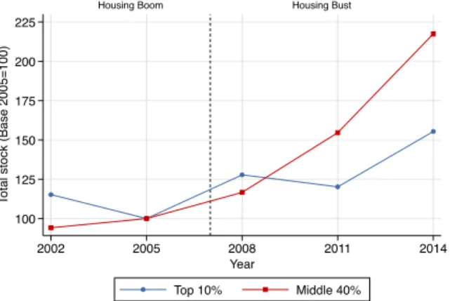
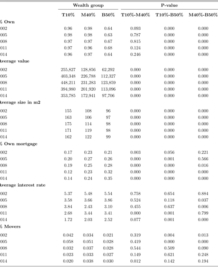
Real estate market dynamics could be a competing explanation for the larger portfolio reshuf-fling among top wealth holders during housing busts. Both housing demand and housing prices could evolve differently across time and space affecting wealth groups in an heterogeneous man-ner. If the dynamics of the real estate market are such that there is a higher demand for the type of properties owned by top wealth holders during the housing bust, this could explain why they managed to dissave more in real estate. Using wealth surveys, I document that indeed primary residences and other properties owned by bottom and middle wealth holders have different char-acteristics (e.g., value, size) than properties owned by the top. However, using information (e.g., number of listings, number of contacts received by listing, offer price) on the universe of 2009 property listings from the largest Spanish commercial real estate website, I find that the demand for housing was not significantly different in districts with the highest average house price versus the rest of districts.3 Furthermore, top wealth holders might have decided to dissave relatively more in housing than middle and bottom wealth holders if the value of their properties had not declined or had declined less. Nonetheless, I show that top wealth holders live in municipalities whose average house price has experienced a similar evolution to municipalities in which bottom and middle wealth holders reside. This evidence suggests that real estate market dynamics are not driving the differential saving behavior across wealth groups during housing busts.
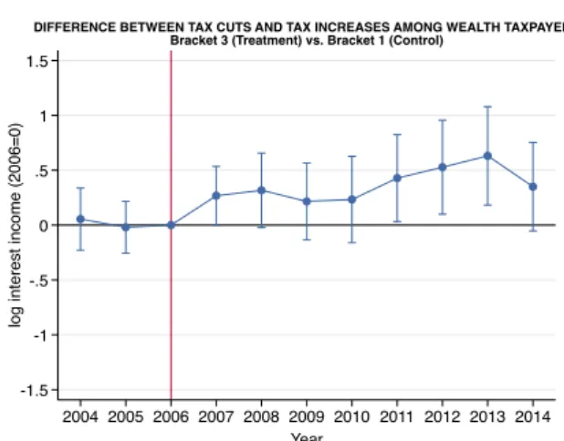
I also document that institutional factors such as tax incentives can exacerbate differences in saving behavior along the wealth distribution. In particular, I examine a large reform introduced in 2007 on the Spanish personal income tax aimed at incentivizing saving on financial assets. Financial income (i.e., interest, dividends, short-term capital gains) that used to be taxed under a progressive tax schedule with the rest of income components, started to be taxed at a flat rate of 18%. The reform implied substantial tax variation across individuals, largely benefiting top
3The demand index I use is directly elaborated by the commercial real estate company (El Idealista). It is based
on the number of e-mails received by listing normalized by a factor, to make it comparable across space and time.
wealth holders. Using a novel personal income and wealth tax panel, I exploit quasi-experimental variation created by the reform to estimate behavioral responses to the Spanish personal income tax in a differences-in-differences setting. I compare the evolution of reported interest income for individuals who experience a tax cut (treatment group) with individuals who experience a slight tax increase (control group) after the reform.4 I find that interest income increased on average 76% more for individuals who experienced a tax cut relative to those who experience a slightly tax increase. The effect is increasing with the size of the tax cut. Counterfactual simulations with the wealth distribution series reveal that the capital income tax reform explains on average 60% of the growth rate in the top 10% wealth share during the recent housing bust. In conjuction, these analyses suggest that portfolio adjustment frictions appear to be the most plausible explanation for the differential saving behavior across wealth groups during housing busts and that behavioral responses to tax incentives can exacerbate this behavior.5
This paper contributes to four main literatures. First, there is a nascent theoretical and em-pirical literature analyzing the determinants of wealth inequality dynamics (Bach et al. [2018a],
Bach et al.[2018b],Fagereng et al.[2019a],Fagereng et al.[2019b],Gomez[2019],Hubmer et al.
[2019],Kuhn et al.[2018]). While these studies have mainly focused on the implications of asset prices and rates of return for wealth inequality, my results reveal that behavioral components, and in particular saving responses, are also important factors behind wealth inequality dynam-ics. To my knowledge, this is the first study documenting how changes in the composition of savings across wealth groups shape the wealth distribution over the business cycle. Moreover, these studies have barely documented or explained why saving rates change in the way they do. This paper moves one step forward and uses quasi-experimental evidence from a large Spanish reform to quantify for the first time by how much capital income tax cuts contribute to changes in saving behavior and wealth concentration.
Second, this work also relates to the literature measuring wealth distributions (Alvaredo et al. [2018a], Garbinti et al. [2018a], Kopczuk and Saez [2004], Kuhn et al. [2018], Roine
4I focus on interest because dividends and capital gains are quite volatile and even more so during the crisis, so
that any type of saving response is very hard to identify.
5I also briefly discuss other candidate explanations: differences in risk aversion, financial literacy, financial
advi-sory and expectations on house prices. First, using Spanish wealth surveys I show that the fraction of households reporting not to be willing to take any financial risk is significantly lower for the top 10% wealth group relative to the middle 40% wealth group and even lower relative to the bottom 50% wealth group. Second, using a Spanish survey of financial competences I document that both financial knowledge and independent financial advising are positively correlated with economic outcomes, such as income. Thus, top wealth holders might have reshuffled their portfolio more during the housing bust because they were less risk averse or more financially informed. Nonetheless, differences in risk aversion, financial knowledge and financial advising seem to only explain why bottom and middle wealth holders did not invest as much as top wealth holders in risky financial assets (i.e., stocks), but not why they did not invest as much on safe financial assets (i.e., deposits). Little financial knowledge or advice is needed to invest in safe financial assets, especially deposits. Third, top wealth holders could have also dissaved more in housing if they had more pessimistic expectations about the future evolution of house prices. However,Bover[2015] finds using survey data no significant association of such beliefs with wealth during the recent housing bust.
and Waldenström [2009], Saez and Zucman [2016], Smith et al. [2019]). These studies have
documented long-term wealth inequality trends, but abstracting from cyclical effects. This
paper is the first to provide comprehensive long-term evidence on how housing booms and busts
shape the wealth distribution. Kuhn et al. [2018] have recently shown that housing booms
lead to substantial wealth gains for leveraged middle-class households in the US. However, the extent to which this pattern persists or not throughout housing busts has received much less attention so far. In Spain, the wealth distribution has been analyzed in the past using wealth tax records (Alvaredo and Saez [2009]) and wealth survey data (Anghel et al. [2018]), but the coverage in terms of distribution and time span was limited. The new wealth distribution series constructed in this paper covers the full distribution over the period 1984-2015 and provides complete long-run evidence on the evolution of wealth inequality over the last four decades in Spain.
Third, I also contribute to the literature studying how inequality evolves over the business cycle (Barlevy and Tsiddon [2006], Bonhomme and Hospido [2017], Castañeda et al. [1998],
Heathcote et al. [2010], Kuznets and Jenks [1953], Storesletten et al. [2004]). These studies find that income inequality is countercyclical—with some exceptions at the top of the income distribution—but they do not analyze the implications of cyclical effects for wealth inequality.6 This paper shows that wealth inequality is also countercyclical in the context of housing booms and busts.
Finally, this study contributes to the literature on housing and portfolio choice (Campbell
[2006], Chetty et al. [2017], Cocco [2004], Guiso et al. [2002]). These studies analyze the role played by housing in the portfolio decisions of households, but they abstract from the implications of these decisions for wealth inequality. The results of this paper emphasize the importance of portfolio choice and in particular, differences in portfolio rebalancing across wealth groups, in shaping wealth inequality dynamics.
The layout of the paper is as follows. Section II discusses the concepts, data and methodology used to construct the wealth distribution series. In Section III, I first present the main patterns in real house prices and aggregate wealth and I then analyze wealth inequality dynamics during housing booms and busts. Lastly, I develop a new asset-specific decomposition of wealth accu-mulation and carry some siaccu-mulation exercises to understand the key drivers of the dynamics of wealth inequality during housing booms and busts. In Section IV, I propose and explore several candidate explanations for the observed asset-specific saving responses. In Section V, I reconcile and test the methodology used with other sources. Finally, Section VI concludes.
II
Concepts, Data and Methodology
This section describes the concepts, data and methodology used to construct the Spanish wealth distribution series over the period 1984-2015, which will then be used to study the implications of housing booms and busts for wealth inequality. Further methodological details of the Spanish specific data sources and computations can be found in the appendix at the end of the paper and all detailed calculations in the companion data appendix.
II.I
Aggregate Wealth: Concept and Data Sources
The wealth concept used is based upon national accounts and it is restricted to net household wealth, that is, the current market value of all financial and non-financial assets owned by the household sector net of all debts. For net financial wealth, that is, for financial assets net of liabilities, I rely on the latest and previous financial accounts (European System of Accounts (ESA) 2010 and 1995, Bank of Spain) for the period 1996-2015 and 1984-1995, respectively. Financial accounts report wealth quarterly and I use mid-year values.
Households’ financial assets include equities (stocks, investment funds and financial deriva-tives), debt assets, cash, deposits, life insurance and pensions. Households’ financial liabilities are composed of loans and other debts. It is important to mention that pension wealth excludes Social Security pensions, since they are promises of future government transfers. As stated in
Saez and Zucman[2016], including them in wealth would thus call for including the present value of future health care benefits, future government education spending for one’s children, etc., net of future taxes. Hence, it would not be clear where to stop.
The wealth concept used only considers the household sector (code S14, according to the System of National Accounts (SNA)) and excludes non-profit institutions serving households (NPISH, code S15). There are three reasons which explain this decision. First, due to lack of data, non-profit wealth is not easy attributable to individuals. Second, income from NPISH is not reported in personal income tax returns. Third, non-profit financial wealth amounts to
approximately 1-3% of household financial wealth between 1995 and 2017 in Spain (TableA1).
Hence, it is a negligible part of wealth and excluding it should not alter the results.
Spanish financial accounts report financial wealth for the household and NPISH sector and also for both households and NPISH isolated as separate sectors. However, the level of disaggre-gation of the balance sheets in the latter case is lower than in the case in which households and NPISH are considered as one single sector. For instance, whereas the balance sheet of the sector of households and NPISH distinguishes among wealth held in investment funds and wealth held in stocks, the balance sheet of the household sector only provides an aggregate value with the sum of wealth held in these two assets. In order to have one value for household wealth held in investment funds and one value for household wealth held in stocks, I assume that they are
proportional to the values of households’ investment funds and stocks in the balance sheet of households and NPISH.
For non-financial wealth, it is not possible to rely on non-financial accounts based on the SNA. Even though there are some countries that have these accounts, such as France and United King-dom, no institution has constructed these type of statistics for Spain yet. I need to use other statistics instead. My definition of household non-financial wealth consists of housing and un-incorporated business assets and I rely on the series elaborated by Artola Blanco et al. [2019]. Housing wealth is derived based on residential units and average surface from census data on the one hand, and average market prices from property appraisals, on the other hand.7 Unincor-porated business assets have been constructed using the five waves of the Survey of Household Finances (2002, 2005, 2008, 2011, 2014) elaborated by the Bank of Spain and extrapolated back-wards using the series of non-financial assets held by non-financial corporations also constructed by the Bank of Spain.8
I exclude collectibles since they amount to less than 1% of total household wealth and they are not subject to the personal income tax. Furthermore, consumer durables, which amount to approximately 10% of total household wealth, are also excluded, because they are not included in the definition of wealth by the SNA and there are no statistics about consumer durables owned by Spanish households for the period prior to 2002.9
II.II
Distribution of Wealth: The Mixed Capitalization-Survey
Ap-proach
The wealth distribution series are constructed by allocating the total household wealth as defined in the previous subsection to the various groups of the distribution. I proceed with the following three steps. First, the distribution of taxable capital income is calculated. Second, the taxable capital income is capitalized. Third, I account for wealth that does not generate taxable income. This is a mixed method and not the pure capitalization technique, because income and wealth surveys are used in order to account for both income at the bottom of the distribution and assets that do not generate taxable income.
7Net housing wealth is the result of deducting real estate debt from household real estate wealth. Note that
real estate debt is approximated by total household liabilities. This a quite reasonable approximation since as Table A2in appendix shows, real estate property debt accounts for 80-88% of total household debt over the period 2002-2014 according to the Survey of Household Finances.
8A detailed explanation of the sources and methodology used in order to construct these two series can be found
in the appendix ofArtola Blanco et al.[2019].
9The shares of both collectibles and consumer durables over total household wealth are obtained using the Survey
II.II.I The Distribution of Taxable Capital Income
The starting point is the taxable capital income reported on personal income tax returns. I use micro-files of personal income tax returns constructed by the Spanish Institute of Fiscal Studies (Instituto de Estudios Fiscales (IEF)) in collaboration with the State Agency of Fiscal Adminis-tration (Agencia Estatal de Administración Tributaria (AEAT)). Three different databases are available: two personal income tax panels that range from 1982-1998 and 1999-2014, respec-tively, and personal income tax samples for 2002-2015. For the benchmark series, I use the first income tax panel for 1984-1998, the second panel for 1999-2001 and all income tax samples for 2002-201510. I also use the full second panel 1999-2014 to carry robustness checks. The micro-files provide information for a large sample of taxpayers11, with detailed income categories and an oversampling of the top. The income categories I use are interest, dividends, effective and imputed housing rents, as well as the profits of sole proprietorships.12 The micro-files are drawn from 15 of the 17 autonomous communities of Spain, in addition to the two autonomous cities, Ceuta and Melilla. Two autonomous regions, Basque Country and Navarre, are excluded, as they do not belong to the Common Fiscal Regime (Régimen Fiscal Común), because they manage their income taxes directly. Combined these two regions represent about 6-7% and 8% of Spain in terms of population and gross domestic product, respectively (Tables A4 and A5).
The unit of analysis used is the adult individual (aged 20 or above), rather than the tax unit. Splitting the data into individual units has on the one hand the advantage of increasing comparability as across units since individuals in a couple with income for example at the 90th percentile is not as well off as an individual with the same level of income. On the other hand, it is also more advantageous for making international comparisons, given that in some countries individual filing is possible (i.e. Spain, Italy) and in others (i.e. France, US) not. Since in personal income tax returns the reporting unit is the tax unit, I need to transform it into an individual unit. A tax unit in Spain is defined as a married couple (with or without dependent children aged less than 18 or aged more than 18 if they are disabled) living together, or a single adult (with or without dependent children aged less than 18 or aged more than 18 if they are disabled). Hence, only the units for which the tax return has been jointly made by a married couple need to be transformed. For each of these units I split the joint tax returns into two separate individual returns and assign half of the jointly reported capital income to each
10Even though the first panel is available since 1982, I decided to start using it from 1984 since I found some
inconsistencies between the files for 1982 and 1983 and subsequent years.
11Personal income tax samples are more exhaustive (i.e. 2,700,593 tax units in 2015) than the panels (i.e. 390,613
tax units in 1999). This is the reason why I rely on the tax samples for constructing the benchmark series.
12Note that imputed housing rents exclude primary residence from the period 1999-2015. I explain the way in
which I account for primary residence in the following subsection. Moreover, profits of sole proprietorships are considered as a mixed income, so that I assume as it is commonly done in the literature that 70% of profits are labor income and 30% capital income.
member of the couple.13 In 2015, for instance, this operation converts 19,480,423 tax units into 22,945,329 individual units in the population aged 20 or above, that is, approximately 18% of units are converted.14
One limitation of using personal income tax returns to construct income shares in the Spanish case is that not all individuals are obliged to file. There exist some labor income and capital income thresholds under which individuals are exempted from filing. In 2015, for instance, the labor income threshold when receiving labor income from one single source was 22,000 euros and 12,000 euros when receiving it from two or more sources. The capital income threshold was 1,600 euros for interest, dividends and/or capital gains and 1,000 euros for imputed rental income and/or Treasury bills.15 For instance, over the period 1999-2015, approximately one third of the adult population was exempted from filing (TableA6). I account for the missing adults by first calculating the difference between the population totals by age and gender of the Spanish Population Census with the population totals of the micro-files. I then create new observations for all the missing individuals. By construction, my series perfectly match the Population Census
series by gender and age.16 These new individuals, although being the poorest since they do
not have to file the personal income tax, earn some labor and also some capital income. Hence, we need to account for this missing income, otherwise we would be overestimating the amount of wealth held by the middle and top of the distribution. For that, I rely on the Survey of Household Finances for the period 1999-2015 and on the Household Budget Continuous Survey for the period 1984-1998. AppendixA.I explains in detail the imputation method followed using the two surveys. In Section V, different tests are run to prove the accuracy and robustness of the imputation method.
Finally, before capitalizing the capital income shares, it is important to make sure that in-come is distributed in a coherent way and that there are no significant breaks across years due to, for instance, tax reforms or the use of different data sources. If already the income data are not coherently distributed, neither the wealth distribution estimates will be. In appendixB.I, I explain in detail the particular aspects of the reforms which could potentially affect my method-ology and how I deal with them in order to ensure consistency in the series across the whole
13Since business income from self-employment is a mixed income, only the part corresponding to capital income
is split among the couple.
14Given the incentives of the tax code to file separately whenever both individuals in the couple receive income—
the reductions for filing jointly usually do not compensate for the increase in the tax base—there are more married couples filing individually the further we move up in the income distribution. The 2015 Spanish Personal Income Tax Guide (Guía de la Declaración de la Renta 2015 ) includes a more detailed explanation in Spanish about how personal income tax filing works in Spain.
15In the 2015 Spanish Personal Income Tax Guide (Guía de la Declaración de la Renta 2015 ) the Spanish Tax
Agency includes a more detailed explanation in Spanish about how personal income tax filing works in Spain for tax year 2015.
16The oldest personal income tax panel that I use for the period 1984-1998 does not include information about
age nor gender. Hence, for this period of time I simply adjust the micro-files to match the Population Census totals excluding Basque Country and Navarre but without taking age and gender into consideration.
period of analysis.
II.II.II The Income Capitalization Method
In the second step of the analysis the investment income approach is used. In essence, this method involves the application of a capitalization factor to the distribution of taxable capital income to arrive to an estimate of the wealth distribution.
The income capitalization method used in this paper may be set out formally as follows. An individual i with wealth w invests an amount aij in assets of type j, where j is an index of the
asset classification (j = 1, .., J ). If the return obtained by the individual on asset type j is rj17,
his investment income by asset type is:
yij = rj ∗ aij (1)
and his total investment income:
yi = J
X
j=1
rj∗ aij (2)
Rearranging equation (1), the wealth for each individual by asset type is, thus, the following:
aij =
yij
rj
(3)
By rearranging equation (2), the total wealth for each individual is:
wi = J X j=1 yij rj (4)
In the following paragraphs, I explain how this formal setting is applied to the Spanish case in order to obtain the wealth distribution series.
There are five categories of capital income in personal income tax data: effective and imputed rental income (excluding primary residence since 1999), business income from self-employment, interest and dividends. Tax return income for each category is weighted to match aggregate
national income from National Accounts. I then map each income category (e.g. business
income from self-employment) to a wealth category in the Financial Accounts from the Bank of Spain (e.g. business assets from self-employment).18
As it was mentioned in the previous subsection, income tax data exclude the regions of
17Note that the capitalization method relies on the assumption that the rate of return is constant for each asset
type, that is, it does not vary at the individual level.
18Capital gains are excluded from the analysis. The reason is that they are not an annual flow of income and
consequently, they experience large aggregate variations from year to year depending on stock price variations. By including them, the fluctuations in the wealth distribution series could be biased since we observe large variations in capital gains from year to year.
Basque Country and Navarre. Therefore, before mapping the taxable income to each wealth category, income and wealth in national accounts need to be adjusted to exclude the amounts corresponding to these two regions. Ideally, if one would know the amount of wealth and income in each category by region, one could simply discount the wealth and income corresponding to these two regions. Unfortunately, neither the Bank of Spain nor the National Statistics Institute have constructed regional national accounts with disaggregated information by asset type yet, so another methodology needs to be used. I assume that income and wealth in each category are proportional to total gross domestic product and housing wealth excluding these two regions, respectively.19
Once income and wealth have been adjusted, a capitalization factor is computed for each category as the ratio of aggregate wealth to tax return income, every year since 1984. In 2015, for instance, business income accounts for about 20.6 billion euros and business assets from self-employees for 575.6 billion euros. Hence, the rate of return on business assets is 3.6% and the capitalization factor is equal to 27.9. Flow returns (and thus capitalization factors) vary across asset types, being for most of the period higher for financial assets than for business assets and housing (Table1).20 This is consistent with the findings ofJordà et al.[2019], who show that the rate of return on equities has outperformed on average the rate of return on housing since the 1980s, but not in previous decades. This procedure ensures consistency with aggregate national income and wealth accounts. Having wealth distribution series which take all aggregated wealth into account is specially relevant for the purpose of this paper, which is to understand how periods of large changes in housing prices shape the entire wealth distribution.
The capitalization method is well suited to estimating the Spanish wealth distribution because the Spanish income tax code is designed so that a large part of capital income flows are taxable. However, as it has been already mentioned, tax returns do not include all income categories. In the following subsection, I carefully account for the assets that do not generate taxable income.
19As it has already been mentioned, total gross domestic product in Basque Country and Navarre accounts for
approximately 8% of total gross domestic product over the period 1984-2016 (TableA5). This assumption seems reasonable since the share of housing wealth in Basque Country and Navarre also amounts to approximately 8% of total housing wealth (Table A7).
20The rate of return on housing using National Accounts is very low for international standards, particularly
during the most recent period (2002-2015). This can be explained by the fact that differences in housing wealth growth versus housing rental income growth were much larger in Spain than in the rest of advanced economies. One potential explanation are the large differences in demand for renting (low) versus buying (high) dwellings in Spain, which have led to a larger increase in housing versus rental prices. In fact, the home-ownership ratio for primary residences is approximately 80% according to the 2011 Census of dwellings (INE) and the calculations of the Bank of Spain (TableA8). One cannot, however, fully disregard the existence of some type of measurement error in the construction of the rental income and/or housing wealth series. Nonetheless, the methodology used in this paper relies on the assumption of equal returns by asset class along the wealth distribution and in Section V I show that this is a plausible assumption in the Spanish context. Hence, if there exists some type of measurement error, it should not alter the wealth distribution series.
II.II.III Accounting for Wealth that Does not Generate Taxable Income
The third and last step consists of dealing with the assets that do not generate taxable income. In Spain, there are four assets whose generated income is not subject to the personal income tax: Primary residences21, life insurance, investment and pension funds.22 Although these assets account for a large part of total household wealth, namely around 40-50% of total net household
wealth (Table A9), the fact that they do not generate taxable income does not constitute a
non-solvable problem for one main reason: Spain has a high quality wealth survey, the Survey of Household Finances (SHF).
As it was mentioned in the beginning of this section, this survey is elaborated every three years since 2002 by the Bank of Spain. It provides a representative picture of the structure of incomes, assets and debts at the household level and does an oversampling at the top. This is achieved on the basis of the wealth tax through a blind system of collaboration between the National Statistics Institute and the State Agency of Fiscal Administration, which preserves stringent tax confidentiality. The distribution of wealth is heavily skewed and some types of assets are held by only a small fraction of the population. Therefore, unless one is prepared to collect very large samples, oversampling is important to achieve representativeness of the population and of aggregate wealth and also, to enable the study of financial behavior at the top of the wealth distribution. Hence, this survey is extremely suitable for this analysis and it allows to allocate all the previous assets on the basis of how they are distributed, in such a way as to match the distribution of wealth for each of these assets in the survey. AppendixA.II
explains in detail the imputation method used relying on the survey, which is very similar to the one developed by Garbinti et al.[2018b] for France.
To make sure that the imputations are correctly done, in Section V I have carried different robustness checks using the Survey of Household Finances. The levels and composition of my series are almost identical to the ones obtained using the direct reported wealth from the survey.
III
How do Housing Booms and Busts Shape the Wealth
Distribution?
This section presents the main results of the paper. The first subsection describes the evolu-tion of real house prices and aggregate household wealth in Spain over the period 1984-2015
21Imputed rents on primary residence are exempted since 1999. Hence, I only need to impute primary residence
for the period 1999-2015.
22Unreported offshore assets do also not generate taxable income. Following Alstadsæter et al. [2019], I
re-calculate the wealth distribution series accounting for unreported offshore assets by assigning proportionally to the top 1% wealth group the annual estimate of unreported offshore wealth of Artola Blanco et al. [2019]. Due to the uncertainties related to these calculations, I do not include offshore assets in my benchmark series. Appendix D describes the methodology used to account for unreported offshore assets in detail and presents the adjusted wealth distribution series.
and identifies the different housing booms and busts episodes. The second subsection docu-ments the wealth inequality fluctuations and uses a new asset-specific decomposition of wealth accumulation to better understand the observed dynamics during house price cycles.
III.I
Evolution of Real House Prices and Aggregate Household Wealth
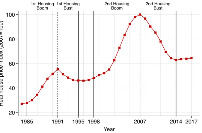
Spain is an ideal laboratory to understand the implications of housing booms and busts for wealth inequality for three main reasons. First, the country has experienced two house price cycles over the period 1984-2015, which makes it possible to analyze in detail the implications of large asset price changes for wealth inequality taking a long-term perspective. The first house price cycle started in 1984 and ended up in 1995, with 1991 as turning point. The second house price cycle started in 1996 and finished in 2014, with 2007 as turning point. Housing booms and busts are house price cycles in which house price growth is considered large enough. There is no consensus about the threshold that needs to be chosen. In this paper, I will follow a similar approach to
International Monetary Fund [2009] and identify housing boom and busts as periods when the four-quarter moving average of the annual growth rate of real housing prices falls above (below) 2.5%. According to this methodology, Spain had two housing booms (1985-1991, 1998-2007) and
two housing busts (1991-1995, 2007-2014) during this period of time (Figure 1). Appendix C
discusses alternative methodologies that have been used to identify housing booms and busts. No matter which methodology is used results are very similar.
Second, the dimensions of the two house price cycles were quite different. Whereas during the first and second boom housing prices rose on average 11.6% and 11.8% by year, respectively, the decline in house prices was larger during the recent housing bust (5.7% on average by year) than during the old housing bust (3.6% on average by year). Moreover, the rise in total real estate transactions was much larger during the second episode than during the first one (Figure A3a). The larger increase was partly due to an increase in the stock of new dwellings (Figure A3b), many of which were acquired through mortgage loans (FigureA3c). Moreover, the recent housing bust happened together with an economic crisis and a stock market crash, whereas there was no stock market collapse nor economic crisis at the turning point of the old housing boom.23 This heterogeneity across the two episodes is useful to understand the implications of housing booms and busts for wealth inequality under different economic scenarios and house price cycle intensities.
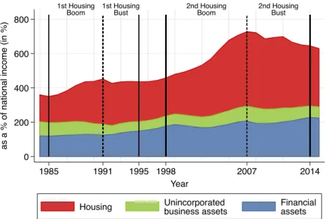
Third, Spain reached an unprecedented level in its household wealth to national income ratio, almost doubling during this period of time. Household wealth amounted to 359% in 1984 and it grew up during the first housing boom up to 435% in the early 1990s. During the housing
23Spain went under a profound economic crisis during the 1990s but it did not start until 1993 and ended up in
bust of the mid-1990s it stabilized and from 1998 onwards, it started to increase more rapidly reaching the peak of 727% of national income at the end of the second housing boom in 2007. After the burst of the crisis in 2008, it dropped and it has been decreasing since then. In 2015, the household wealth to national income ratio amounted to 629%, a level which is similar to the wealth to national income ratio of 2004, but much higher than the household wealth to national
income ratios of the 1980s and 1990s (Figure 2a). The level of household wealth to national
income that Spain reached in 2007 is the highest among all countries with available records in the early twenty-first century (Figure2b).
III.II
Wealth Inequality Dynamics during Housing Booms and Busts
The high level of disaggregation of the Spanish wealth distribution series, together with the existence of the two housing boom-busts episodes, allows me to carry the first comprehensive long-term study on how housing ups and downs shape the wealth distribution.
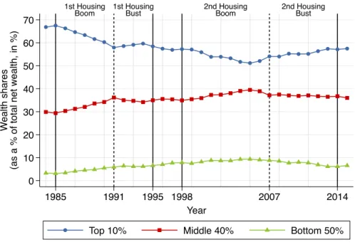
Figure 3a displays the wealth distribution in Spain over the period 1984-2015 decomposed
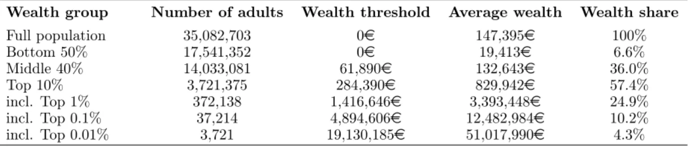
into three groups: top 10%, middle 40% and bottom 50%. The wealth share going to the bottom 50% has always been very small ranging from 3 to 10%, the middle 40% has concentrated between 29% and 40% of total net wealth and the top 10% between 51% and 68% over the period of analysis. Wealth levels, thresholds and shares for 2015 are reported on Table2. In 2015, average net wealth per adult in Spain was about 150,000 euros. Average wealth within the bottom 50% of the distribution was slightly less than 20,000 euros and their wealth share was 6.4%. Average wealth within the next 40% of the distribution was slightly more than 132,000 euros and their wealth share was 36%. Finally, average wealth within the top 10% was nearly 830,000 euros (i.e. about 5.6 times average wealth) and their wealth share was 57.4%.
In terms of long-term dynamics, Figure3ashows that top 10% wealth concentration followed a decreasing trend since the 1980s that reverted at the the beginning of the 2000s. This decline happened at the expense of wealth gains for both middle and bottom wealth groups. Focusing on the dynamics during the two house price cycles, I find that top 10% wealth concentration decreased during the two housing boom episodes and increased during the two housing busts. Both bottom—to a low extent—and middle—to a large extent—wealth holders benefit from housing booms. Contradictory movements in relative asset prices have an important impact on the dynamics of the wealth distribution because asset composition is very different across
wealth groups. As it is shown on Figure 3b, bottom deciles of the distribution own mostly
financial assets in the form of cash and deposits, whereas primary residence is the main form of wealth for the middle of the distribution in 2015. As we move toward the top 10% and the top 1% of the distribution, unincorporated business assets, secondary owner-occupied and tenant-occupied housing gain importance, and financial assets (mainly equities) gradually become the dominant form of wealth. The same general pattern applies for the period 1984-2015, except that
unincorporated assets have lost importance over time, due mainly to the reduction in agricultural activity among self-employees.24
When decomposing the evolution of the wealth shares going to the bottom 50%, middle 40%, top 10% and top 1% by asset class, the impact of asset price movements on wealth shares, particularly the impact of the 2000 stock market boom and the 2007 housing bust, are clearly captured (Figure 4). One particularity of the Spanish case is that housing constitutes a very important asset in the portfolio of households even at the top of the distribution. This has been the case during the whole period of analysis, but it has become more striking in the last fifteen years due to the increase in the value of dwellings. For instance, whereas in 2012 the top 10% and 1% of the wealth distribution in Spain own 26% and 9% of total net wealth in housing, respectively, in France these figures are 19% and 5%, respectively (Garbinti et al. [2018a]).25
The negative correlation between wealth concentration and housing expansions and the pos-itive correlation during housing busts seems to hold in other countries too. Figure A5adepicts the real house price index in Spain, France and the US. All three countries experienced a housing expansion over the period 1998-2007, but the length and dimension of the housing contraction
after 2007 was quite different across the three countries. Figure A5b shows the evolution of
the top 10% wealth share in these three countries. Wealth concentration was higher in Spain than in the US during the 1980s, but since the 1990s trends have diverged. In Spain, top 10% wealth concentration declined and has converged to the levels of the rest of Western European countries such as France (Garbinti et al. [2018a]). In contrast, wealth concentration in the US has been steadily increasing since the late 1980s and it is currently much higher than in conti-nental Europe. In line with the findings for Spain, both in France and the US the evolution of 10% wealth concentration is different during housing expansions and contractions. The top 10% wealth share stabilized in the US and declined in France during the 1998-2007 housing expansion and increased during the housing contraction.
Kuhn et al. [2018] also document using long-term survey data that housing booms lead to substantial wealth gains for leveraged middle-class households and tend to decrease wealth inequality in the US. However, the extent to which these dynamics are purely mechanical or not is still an open question which I address in the next subsection.
III.III
An Asset-Specific Decomposition of Wealth Accumulation
The drop in wealth inequality during booms and the increase during busts would be mechanical if all individuals kept their portfolio composition fixed—that is, they did not sell any of their
24Equities include both listed and non-listed equities and that non-listed equities include incorporated business
assets.
25The Spanish wealth distribution series can be also decomposed by age over the period 1999-2015. AppendixE
assets nor buy or acquire new assets—so that the decline and increase would be entirely explained by differences in capital gains along the distribution. During housing booms, capital gains on housing are usually larger than on financial assets. Consequently, because the middle and bottom of the wealth distribution have a larger share of housing in their portfolio than the top, they experience larger wealth gains, all else equal. On the contrary, during housing busts, capital gains on housing tend to fall more than on financial assets. As a result, because the middle and bottom of the wealth distribution have a larger share of housing in their portfolio than the top, they experience larger wealth losses, all else equal. Table1shows that indeed capital gains on housing were larger than on financial assets during both housing booms and lower than on financial assets during both housing busts in Spain.
The aim of this section is thus to analyze which are the underlying forces driving the dynamics of wealth inequality during housing booms and busts and quantify its importance. Are the observed dynamics entirely due to differences in capital gains or are there any other forces (i.e., labor income, saving rates) driving the dynamics? To answer this question, my starting point is to decompose the wealth distribution series using the following transition equation:
Wt+1g = (1 + qgt)[Wtg+ sgt(YLgt + rgtWtg)], (5)
where Wtg stands for the average real wealth of wealth group g at time t, YLgt is the average real labor income of wealth group g at time t, rgt the average rate of return of group g at time t, qgt the average rate of real capital gains of wealth group g at time t26 and sg
t the synthetic saving
rate of wealth group g at time t. By convention, savings are assumed to be made before the asset price effect qtg is realized. The saving rate is synthetic because the identity of individuals in wealth group g changes over time due to wealth mobility.
I follow the same approach as Garbinti et al. [2018a] and Saez and Zucman [2016] and
calculate the synthetic saving rates that can account for the evolution of average wealth of each group g as a residual from the previous transition equation. This is a straightforward calculation since I observe variables Wtg, Wt+1g , YLgt, rtg and qtg over the whole period 1984-2015. Hence, the three forces that can affect the dynamics of wealth inequality are inequality in labor incomes, rates of return and saving rates.
In this paper, I go one step forward and develop a new asset-specific wealth accumulation decomposition by breaking down the previous transition equation by asset class: net housing, business assets and financial assets.27 The transition equation is as follows:
26Real capital gains are defined as the excess of average asset price inflation, given average portfolio composition
of wealth group g, over consumer price inflation.
27Artola Blanco et al. [2019] do a similar decomposition to analyze the dynamics of aggregate wealth in Spain,
Wt+1g = WH,t+1g + WB,t+1g + WF,t+1g , (6) where WH,t+1g = (1 + qtg)[WH,tg + sgH,t(YLg t + r g tW g H,t)] (7) WB,t+1g = (1 + qgt)[WB,tg + sgB,t(YLgt + rgtWB,tg )] (8) WF,t+1g = (1 + qtg)[WF,tg + sgF,t(YLg t+ r g tW g F,t)] (9)
This new asset-specific wealth decomposition allows me to quantify not only the relative importance of each channel, but also the role played by each asset in explaining the saving dynamics along the wealth distribution. By construction, the sum of the saving rates in equations 7-9 adds up to the total saving rate for wealth group g. This decomposition is critical for my purpose of understanding how housing booms and busts shape the wealth distribution. The reason is that during these episodes one should expect housing to play a relative more important role than other assets in explaining wealth inequality dynamics.
The first potential force which can drive wealth inequality dynamics is labor income inequal-ity. Figure 5a depicts the evolution of labor income shares for the different wealth groups over the 1984-2015 period. Overall, the evolution of labor income inequality has been quite stable throughout the whole period, with some moderate fluctuations. The middle 40% share declined during the first housing boom and it then remained stable until 2010, after which it started to increase at the expense of the decline in the bottom 50% share. This is consistent with the large increase and high levels of unemployment, specially among the young, during the recent housing bust.28 The top 10% share increased during the mid-1980s and decreased during the beginning of the 2000s, a period of rapid economic growth. Despite these fluctuations, the shares are overall quite stable and there is nothing particular in the observed labor income dynamics which seems to have played an important role in explaining the evolution of wealth inequality during housing booms nor busts.
Rate of return inequality is the second potential force driving wealth inequality dynamics. It might arise due to differences in flow rates of return or real capital gains along the distribution. Figure 5b displays the evolution of flow rates of return and Figure 5c of real capital gains for the different wealth groups over the 1984-2015 period. Rates of return have considerably fallen in the last thirty years, following similar trends across the whole wealth distribution. This is
28According to the Spanish Statistics Institute (INE), the unemployment rate almost tripled between 2007 and
mainly due to the fall in returns on some financial assets, such as interest rates. However, differences in rates of return levels across wealth groups are still quite significant. The further up one moves along the distribution, the higher are the rates of return.29 This is consistent with the large portfolio differences that were previously documented, that is, top wealth groups own more financial assets, such as equities, that have higher rates of return than for instance housing. Persistent differences in rates of return over time across the whole distribution seem to perpetuate the high levels of long-run wealth concentration. Nonetheless, because trends are quite similar across wealth groups, they do not seem to be the main drivers of wealth inequality dynamics during housing booms and busts.
Contrary to flow rates of return, differences in real capital gains along the distribution do seem to considerably change during housing booms and busts (Figure5c). Capital gains increase during housing booms and decline during housing busts across all wealth groups. During housing booms, capital gains are larger for the middle 40% and bottom 50% of the wealth distribution than for the top 10%. The reason is that the middle and the bottom have a larger share of housing in their portfolio than the top and consequently, they benefit more from the larger increase in capital gains on housing relative to financial assets (Table1). In contrast, differences in capital
gains almost fully converge across all wealth groups during housing busts. Figure 6 compares
the evolution of the benchmark top 10% wealth share with the evolution of the simulated top 10% wealth share using the wealth accumulation decomposition and setting the rate of capital gain equal to zero all along the wealth distribution. Differences in capital gains appear to reduce wealth concentration during housing booms but do not seem to explain the reverting evolution during housing busts. These results could be confounded by the existence of stock market booms and busts. For instance, the larger convergence in capital gains across wealth groups during housing busts relative to housing booms could be simply explained because housing busts take place together with stock market crashes, as it happened during the recent episode. Interestingly, rates of capital gain also nearly converged during the old housing bust and there was no stock market collapse.
By construction, differences in capital gains across wealth groups only come from differences in portfolio composition, since the methodology used relies on the assumption of constant rates of capital gain by asset class along the wealth distribution. These results could be biased if rates of capital gain by asset class were different across wealth groups. For financial assets, this is less of a concern for two main reasons. First, as it has already been shown, individuals in bottom wealth groups hold mainly deposits—which do not generate capital gains—so that most capital gains on financial assets are earned by top wealth groups. Second, I use different rates of capital
29Bach et al.[2018b] andFagereng et al.[2019b] also document a positive relationship between returns and wealth
gain for each financial asset class (debt securities, equities, investment funds, life insurance and pension funds) instead of a single rate of capital gain for all financial assets. In contrast, I only rely on one rate of capital gain for housing. This could be a concern if housing price growth was different along the wealth distribution during housing-price cycles.
To show that differences in house prices across wealth groups are modest in this context, I assign to each individual the average house price of the municipality in which they reside. I then
calculate the average house price by wealth group. Figure A6a shows average house prices for
the top 1% and top 10%, middle 40% and bottom 50% wealth groups over the period 2005-2015. Despite the large volatility in house prices during this period of time, the evolution of average house prices has been quite similar across wealth groups. It is only after 2014—when average house prices started to rise for the first time since the end of the housing boom—that house prices across wealth groups have started to diverge. The homogeneity in the evolution of house prices in Spain can also be also seen when comparing the evolution of average house prices between coastal versus non-coastal municipalities (FigureA6b) and between municipalities with different population size (Figure A6c). These results are also in line with Fagereng et al. [2019b], who document that heterogeneity in rates of return is much lower for housing than for most financial assets using Norwegian data.
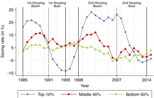
Finally, the third force which can potentially drive wealth inequality dynamics is inequality in saving rates. Figure5ddepicts synthetic saving rates for the top 10%, middle 40% and bottom 50% over the period 1985-2015. Consistent with the high levels of concentration that we observe during this period in Spain, there is a high level of stratification between the top 10%, who save on average 24% of their income annually, and the middle 40% and bottom 50%, who save 10% and 3% of their income on average. These figures are similar to the ones obtained for France and the US (Garbinti et al.[2018a], Saez and Zucman[2016]).
Differences in saving rates across wealth groups increase during booms and decrease during busts. However, contrary to real capital gains, saving rate levels remain higher for the top than for the middle and bottom of the distribution during busts. The stratification in saving rates was more remarkable during the recent episode than during the old one because of differences in the intensity of the house price cycle. The larger increase in saving rates for the top during the recent than during the old boom is mainly due to purchases of secondary residences, both owner-occupied and tenant-owner-occupied housing. As it is shown on Figure A11a, the share of individuals owning a secondary residence rose from 58% to 72% over the period 1998-2007. This is consistent with the large increase in the total number of dwellings transacted during the recent housing
boom, which did not happen during the old episode (Figure A3a). The saving rate for the top
10% wealth group remained at a higher level than for the other wealth groups during the recent housing bust, but it considerably fell. There are two main reasons that explain this drop. First,
both average labor and capital income declined (Figure7). Second, total consumption remained nearly constant (Figure 8a), so that they had to reduce their savings to smooth consumption.
In contrast, saving rates for the middle 40% and bottom 50% declined during the recent housing boom and increased during the bust, contrary to the stability in saving rates for these two groups during the old episode. Middle and bottom individuals also purchased new dwellings.
Figure A11b shows that the middle 40% mainly purchased secondary owner-occupied housing,
since the share of individuals owning secondary owner-occupied housing rose from 25% to 33%
over the period 1998-2007. Figure A11c shows that the homeownership ratio rose from 38%
to 42% for the bottom 50% over the period 1999-2007, mainly due to the purchase of primary
residences.30 However, both middle and bottom individuals acquired their new dwellings by
getting on average highly indebted. Figure 8b depicts the evolution of debt-to-income ratios
by wealth group during the recent house price cycle. Debt-to-income ratio levels significantly differ across wealth groups. They are much higher for the bottom 50% wealth group (100-230%), than for the middle 40% wealth group (38-52%) and the top 10% wealth group (13-24%). The ratio of indebtedness for the bottom 50% experienced the largest changes during the house price cycle. It doubled from 100 to 200% during the housing boom and remained at very high levels during the housing bust. These patterns are also consistent with the large increase in the total number of new mortgage loans attached to real estate during the recent housing boom, which did
not happen during the old episode (Figure A3c). The rise in consumption and in total income
was larger than the saving capacity for the middle 40% and bottom 50% wealth groups, which explains why their saving rates significantly declined over the period 1998-2007. In contrast, the increase in the saving rate for the middle and bottom wealth group during the recent housing bust was due to a drop in consumption to increase savings for prudential reasons (Figure 8a). The drop in consumption for the bottom wealth group was much larger than for the top wealth group, since they also experienced a larger decline in total income, in particular labor income (Figure 7), and they still managed to slightly increase their saving rate.
To better understand the saving patterns of the different wealth groups it is quite useful to look at the composition of the saving rate by asset class, in particular at the share of saving on net housing and on financial assets.31 Figure 9 documents one striking fact: Saving rates on housing and financial assets are much more volatile for the top 10% wealth group than for the middle 40% and bottom 50% wealth groups during housing boom and busts. Saving rates
30The home-ownership ratio keeps growing after 2007. This is most likely due to the fact that many of the
purchased dwellings were actually transacted after 2007 since they were under construction. In fact, FigureA3b
shows that the number of new registered dwellings remain quite high over the period 2008-2010. Another potential explanation for this increase can be mobility along the wealth distribution.
31To simplify the analysis, I do not show the saving rate on unincorporated business assets, since they account on
average for less than 15% of total net household wealth and consequently, they play a minor role in explaining wealth inequality dynamics. This saving rate can be found in the appendix (FigureA7).