HAL Id: hal-02876981
https://hal-pjse.archives-ouvertes.fr/hal-02876981
Preprint submitted on 21 Jun 2020
HAL is a multi-disciplinary open access
archive for the deposit and dissemination of
sci-entific research documents, whether they are
pub-lished or not. The documents may come from
teaching and research institutions in France or
L’archive ouverte pluridisciplinaire HAL, est
destinée au dépôt et à la diffusion de documents
scientifiques de niveau recherche, publiés ou non,
émanant des établissements d’enseignement et de
recherche français ou étrangers, des laboratoires
Examining the Great Leveling: New Evidence on
Midcentury American Inequality
Matthew Fisher-Post
To cite this version:
Matthew Fisher-Post. Examining the Great Leveling: New Evidence on Midcentury American
In-equality. 2020. �hal-02876981�
World Inequality Lab Working papers n°2020/01
Examining the Great Leveling: New Evidence on Midcentury American
Inequality
Matthew Fisher-Post
Keywords : United States; Economic history; Inequality; income inequality;
wage inequality
Examining the Great Leveling: New Evidence on
Midcentury American Inequality
Matthew Fisher-Post
∗†January 2020
Abstract
The mid-20th century American decline in income inequality has been called “the greatest leveling of all time,” despite a similarly unmatched rate of economic growth. To establish this insight, pioneering research has tracked a century of top income shares. However, limitations in the historical data had meant that we still do not fully understand the dynamics of change within the bottom 90% of the income distribution (prior to the 1960s). This paper sheds light on changes within the
mid-dle class—to study early and midcentury trends in income and wage in-equality, by applying a powerful statistical model to archival tax records and survey data. We find that: (i) pre-war economic growth (and reduc-tion in inequality) reached the upper middle class sooner than it (and they) reached the poorest households; and (ii) wartime relative income gains for the poorest were short-lived, while they proved durable for the upper middle class. In short, the relative gains from the New Deal, World War II and postwar eras were both more pronounced and more durable for the upper middle class than for the poorest. However, post-war wage compression lasted 30 years, to the particular benefit of the working poor.
JEL N92, O51, H2, J3
∗World Inequality Lab, Paris School of Economics 48 Boulevard Jourdan, Paris 75014 France
mfp@psemail.eu
†The author gratefully acknowledges research support from the Sloan Foundation and the Franco-American Fulbright Commission—as well as guidance and insight from Facundo Alvaredo, Thomas Piketty and Gabriel Zucman, among many more without whose inputs this project would not have been possible. Errors are mine.
1
Introduction
This investigation will re-examine long-run trends in income distribution in the 20th century United States among the “bottom 90” percent of income earners, by returning to previously unused archival data, by using a new method for statistical inference on this data, and by a series of imputations for problematic missing data,
The foundation for this work, Piketty and Saez’s first (2003) foray painstak-ingly tracked US wealth and income inequality over the 20th century, a series that has since been expanded to include the early 21st century (Saez 2016). Most recently Piketty, Saez and Zucman (2018) harmonized long-run macroe-conomic data with the same tax data and more recent survey estimates, in order to provide an estimate of the full national income distribution, one that includes all sources of income in the national accounts. Taken together, these analyses have helped to both predict and now explain the increasing concen-tration of income at the top of the distribution, as income and wealth inequal-ity in the US have risen to a level not seen since the early 20th century.
This study will attempt to extend the detail found in those later esti-mates, to the earlier era: Where the existing distributional national accounts study for the United States only begins in 1962 (for the full income distribu-tion and not only the top 10 percent), we provide estimates back to 1913 (the beginning of the federal income tax).
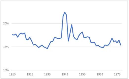
To place this study in the context of the literature from Piketty-Saez (2003) to present, first we show the existing long-run series on American
fis-cal income inequality at the tax unit level (Figure1). Overlaid in blue is a preview of our results.
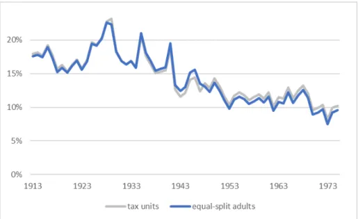
Continuing in the tradition of this literature, after the Piketty-Saez-Zucman (2018) study, we also now observe the top 10% and top 1% shares not only on a tax unit basis, but also since 1962 on the basis of equal-split adults. The concept of equal-split adults (splitting tax-unit income equally among the adults within a tax unit) eliminates any bias in the series that might owe to demographic characteristics, by which high-income earning households (and tax units) might file as a married couple more frequently than low-income households (which would bias the measure or inequality up-ward, if we compare rich couples with poor individuals). Also since 1962, we now know the evolution of middle-class and lowest income shares, including the share of total fiscal income that accrued to the bottom 50% of earners, and that to the 50th to 90th percentiles (what we call the middle 40%). Bot-tom 50% and middle 40% shares are shown below (Figure2) in dark green, while top 10% and top 1% shares are shown in red. The dash line overlay is a preview of our new results.
Figure 1: Top 10% and top 1% fiscal income share, tax units, 1913-2014. Adapted from Piketty-Saez (2003) benchmark series. Blue dash line overlay is a preview of our results.
We extend this innovative historical record back from 1962 to 1913. While Piketty, Saez and Zucman (2018) have estimated the full percentile distribu-tion of US income shares since 1962, this had not yet been done for the years prior to 1962. Nor had this been done for the income from wages and salaries, which is the most significant source of total fiscal income, and especially for middle-class households. Finally, we scale up our inference from fiscal income to pre-tax distributional national accounts.1
The purpose of this study, then, is threefold: (1) to contribute data inter-polation and analysis on the distribution of American income prior to 1962; (2) to place new inferences in the context of what is already known about the
evolution of American income inequality in the 20th century; and (3) to make sense of these observed patterns.
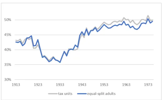
One of our main results can be neatly summarized in Figure3. We ob-serve that the bottom 90 percent share of national income has indeed changed over time, but that the split within the bottom 90 had been relatively sta-ble over the middle of the 20th century. Indeed, as the Piketty-Saez-Zucman study shows, the poorest 50 percent of the population has lost in its share of national income proportionally to the loss of the ”middle” 40 percent (upper middle class, from 50th to 90th percentiles of the income distribution).
1For a more thorough discussion of the income concepts used in this paper, please refer to Alvaredo et al (2016).
Figure 2: Top 10% and top 1%, middle 40% and bottom 50% fiscal income share, equal-split adults, 1913-2014. Adapted from Piketty-Saez-Zucman (2018) benchmark series. Dashed lines preview results.
What the new results now show is that the gains of the poorest 50 per-cent earlier in the per-century were not proportional to the gains of the middle 40 percent. In fact, by the early 2010s the poorest 50 percent had become as poor as they had been at any point in the past century (relatively speak-ing, i.e., as a proportion of the overall ”pie” of national income)–while for the middle 40 percent this was not true. The relative gains from the New Deal, World War II and postwar eras were both more pronounced and have been more durable for the upper middle class than for the poorest. What the mid-century middle class gained, the poorest (proportionally) did not gain; what the late 20th century working poor lost, the middle class (proportionally) did not lose.
Prior to this study, the full picture of early and mid-20th century pat-terns of income distribution had been missing. Data had been the largest constraint. For the early 20th century American economy, Piketty, Saez and Zucman (2018) summarize the missing data issue as follows:
For the pre-1962 period, no micro-files are available so we rely in-stead on the Piketty and Saez (2003, updated to 2015) series of top income shares, which were constructed from annual tabula-tions of income and its composition by size of income (US Trea-sury Department, Internal Revenue Service, annual since 1916). (ibid.)
Regarding these top 10% shares, the earlier paper explains: “Before 1944, because of large exemptions levels, only a small fraction of individuals had to file tax returns and therefore, by necessity, we must restrict our analysis to the top decile of the income distribution” (Piketty Saez 2003).
Until now, the paucity of pre-1962 data has inhibited analysis of early 20th century changes across the whole of the income distribution. However, as total income (national accounts) data was not missing for these years, and since top decile income data was not missing, it was possible to estimate the “top 10” vs. “bottom 90” percent split in the income distribution.
A striking methodological advance allows us to estimate a generalized Pareto curve and “nonparametrically recover the entire distribution based on tabulated income or wealth data as is generally available from tax authori-ties” (Blanchet, Fournier and Piketty 2017). Applied to United States data 1962-2014, the method is shown to closely follow the true distribution using only threshold tabulations. Since this type of tabulation remains the extent of our tax data for the period 1913-1961, in the absence of micro-data tax records, such precision to “smooth” the income density distribution is a wel-come source of new estimation.
Figure 3: Middle 40% (green, above) and bottom 50% (yellow, below) pre-tax national income share, equal-split adults, 1913-2014. Dark shaded areas pre-1962 are new results. Light shaded areas after 1962 are from Piketty-Saez-Zucman (2018).
However, several imputations are necessary for the generalized Pareto interpolation technique to treat our data without bias. First, it is necessary to treat tax units as equal-split adults. Even if the relative distribution of two-income households had not changed over time (it did), tax incentives also could have changed in a way that was heterogeneous across the income distri-bution. The increasing level of households filing tax returns jointly or sepa-rately (whether due to changing incentives, or an increasing number of women in the labor force, or both) could give a misleading impression of middle-class growth if we do not account for the trend by calculating these propensities with greater precision.
A particular challenge in the construction of this dataset will be our treatment of “missing” tax units who did not file tax returns. There are sev-eral approaches we can take to deal with missing data, and we explore two of them. One approach is to assign missing income and missing people to the leftmost side of income distribution, under the (realistic) inference that it is poorer households who do not file tax returns (Saez 2016). Another approach would be to assume that these non-filers were randomly or equally distributed throughout the lower deciles, an approach that is applied with success to French historical income data in Garbinti, Goupille-Lebret and Piketty (2017). We show results from both methods, and ultimately select the former as more appropriate in the context of this data.
An even greater challenge for imputation of missing tax data is in the pre-World War II period, when the majority of American households did not file tax returns—namely, those below the top 10% of the income distribution. To deal with this missing middle-class tax data, we will integrate a historical survey on American family income from 1929-44, harmonized with the tax data. To the extent that they are representative and include reliable informa-tion our “missing” tax units, data from this Goldsmith-OBE series helps us assign the non-missing tax units to their appropriate and realistic rankings in the imputed income distribution—prior to generalized Pareto interpolation the fills in the rest of the cumulative distribution function.
These imputation methods, discussed further below, can be calibrated us-ing post-1962 data: If the survey data distributions match our IRS Statement of Income (SOI) tabulations in the years immediately after 1962, according to micro-data tax records, we can infer that a similar match exists in the years immediately prior to 1962. That inference may be less robust as we move farther into history from this time period, but we pay special attention to changes in pre-World War II survey statistics and federal income tax legisla-tion (cf. Witte 1985) and filing requirements.
Last, we explain the method to move from fiscal income to pre-tax na-tional income, harmonizing tax data with nana-tional accounts to match and distribute 100% of the annual macroeconomic totals from the National Income and Product Accounts.
2
Data and Methodology
Sources
We begin with the same sources as Piketty-Saez (2003) and Piketty-Saez-Zucman (2018). The annual Statement of Income reports of the United States Internal Revenue Service have documented brackets of earned income for the entire taxpaying population since 1916 (and in an earlier version from the Commissioner of Internal Revenue, 1913-15). While micro files (public use sample datasets) are available for the period after 1962, they are not avail-able before, so we revert to meso-level data in tabular form, in which the SOI calculated the number of tax returns and gross income according to stepwise income brackets. These tables were presented each year in similar but not identical formats, with various levels of disaggregation and reformatting, e.g., by specific source of income, by type of tax return, or even by state. Thresh-old levels of tabulated income, categories for inclusion and exemption, and definitions of concepts all fluctuated over time, as did the legislation for tax
filing and taxable status. Nonetheless, we build on the former studies to har-monize a more complete record of fiscal and wage income in the 20th century.
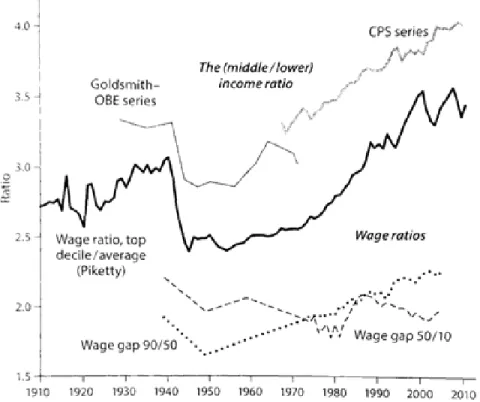
We take advantage of what few sources of information are available on the historical income distribution (see Figure4).
It is clear that there is little information available before World War II (the Census at the time did not ask questions about income). Autor and Goldin, among others (cf. Autor et al 2013; Acemoglu and Autor 2012; Goldin and Katz 2008) have contributed to the literature with studies of US wage trends, but the datasets are either strictly post-1962 (Autor et al 2013) or, at best, have limited explanatory power pre-1940 (Goldin and Katz 2008). Goldin and Katz (2008) made use of occupational wage ratios to draw infer-ences about the evolution of the “skill premium” of white-collar vs. blue-collar jobs, but even if this data is informative, unfortunately it is neither compre-hensive nor does it extend much before World War II. In the present study, we rely primarily on IRS data before complementing it with Goldsmith-OBE survey data for the years before 1945. We will return to discuss that method at the end of this section.
Returning to the IRS archive first of all, then, we produce a dataset with income and wage and filing statistics for the entire register of tax brackets in every year for which the records are available. Beyond the top ten percent of highest-income tax returns, we include every recorded bracket of tax returns, including zero net income, so that we can later analyze the proportion of total income accruing to the bottom 50% of households, and to the “middle” 40% (51st to 90th percentiles of the distribution).
Generalized Pareto curves
The method we use to infer the entire distribution, including below the 90th percentile, is a generalized Pareto curve interpolation (Blanchet, Fournier and Piketty 2017). While the well-known original Pareto distribution function has been taken as roughly appropriate to interpolate the top percentiles of an income distribution (Pareto 1897; Kuznets 1953; Atkinson 2017), Blanchet and Fournier and Piketty developed the nonparametric generalized Pareto curve in order to recover an entire distribution according to varying inverted Pareto coefficients b(p) that are similar but not precisely identical over the course of the smooth distribution function.
Following Fournier (2015) and Atkinson, Piketty and Saez (2011), the Pareto distribution can be expressed as:
F (y) = 1 − (k y)
Figure 4: A catalog of historical income data in the United States, 1910-2010, with findings on inequality ratios (Lindert and Williamson 2016).
where k > 0 is the scale parameter, income is y > k, and α > 1 is the Pareto parameter determining the shape of the distribution. In the classical Pare-tian distribution, the ratio of the average income above y to y itself does not depend on the threshold level of y. This ratio b(p) is the inverted Pareto coef-ficient, given by:
b(p) = a a − 1
While this Pareto coefficient b(p) can be considered as a constant parameter throughout the distribution, it can also be modeled more flexibly to match empirically observed data. This is one of the most interesting contributions of the theory of generalized Pareto curves (Blanchet, Fournier and Piketty 2017), as the technique allows the parameter b(p) to change over the course of the distribution. In turn, this allows us to model an entire income distri-bution based on no more than a few pieces of information sampled from the population: several income levels (e.g., thresholds at cumulative population density p = 10%, 50%, 90% and 99%), and the average income of earners within those brackets. The interpolation method creates a polynomial spline function from these pieces of information. Tests of the method show that an estimation error of less than 1% (on top incomes shares) can be achieved with income information on as little as three brackets, and that the error can be re-duced to less than 0.05% with seven brackets (Blanchet, Fournier and Piketty 2017).
However, the information on these brackets needs to be well placed over the income distribution in order to yield the most precise results. Fortunately, our income data from American tax records after 1944 meets that criterion, and is granular enough to provide information across the entire distribu-tion—for the years in which tax returns are representative of the population (or close to a full population sample). Unfortunately, before 1945, we do not observe a full population sample filing tax returns. We will turn to this ques-tion below. As we will discuss, when we do not have informaques-tion below the 90th percentile, then it is difficult at best (speculative at worst) to infer the levels and shares of income for middle-class earners. Therefore, we must infer or impute as much information as possible about income levels throughout the population, before setting our generalized Pareto curve distribution func-tion to smooth out the cumulative distribufunc-tion funcfunc-tion and rigorously model income shares accruing to the middle-class and poorest households.
In fine, when we model the cumulative distribution function2, we infer
the entire taxpayer income distribution based on available information from tax brackets and complementary information that we have imputed and as-signed accordingly.
Missing income and missing people: two approaches
One of the greatest challenges of this approach, then, is what to infer about missing information: the people and the income that go unreported in the annual SOI tabulations.
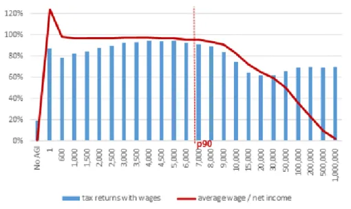
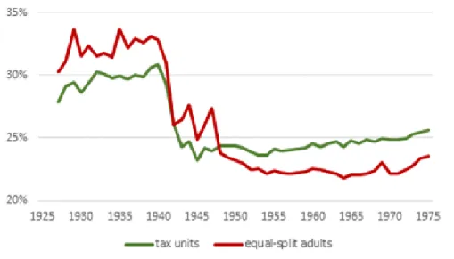
Harmonizing our procedure with the original Piketty-Saez (2003) analy-sis and more recent Piketty-Saez-Zucman (2018) datasets, we know the total number of tax units in the population thanks to US Census and historical data on the marital structure of the population. And from the same source we use the total income of the population (beyond only the tax filers) computed from national accounts data. Piketty and Saez (2003) found that tax return gross income (adjusted gross income, plus transfers, minus capital gains) re-mained between 77 and 83 percent of national accounts’ personal income from 1944 through 1998, after adjustments for non-filers, and imputed this fraction at exactly 80 percent from 1913 to 1944. There were fewer non-filers after 1944, so the amount imputed to non-filers equals only 2-3% of the total income.3 By contrast, non-filers before 1944 represented a much greater
pro-portion of the population (up to 90 percent or more), so the challenge is how to allocate their imputed income across the income distribution. (See Figure
5.)
To determine the full income distribution including non-filers, we will test two approaches. One approach is to simply allocate all missing income on the left side of the income distribution, below a certain threshold where it is assumed that all earners faithfully report their income to the tax authorities. That is the filing threshold of IRS returns. This would not be an unheard-of solution, especially if most unheard-of the unreported income was due to a “filing requirement” below which point of income a person or household was not required to file a tax return.
However, it is possible that this line may be too arbitrary: either (a) many non-filers would be spread along the “true” income distribution even above this amount—and to draw the legal line below which to assign all miss-ing income would be to overestimate the bottom portion of the income distri-bution; or (b), we would be drawing a threshold so high as to be analytically meaningless and lose valuable information about the income distribution be-low that point.
Instead, in a second approach, we could remain agnostic about the rea-sons for non-filing,4and compare another solution: to allocate all missing tax
3After 1945, missing tax units were assumed to average 30% of the non-missing tax units’ average income; they were imputed 50% of that average in 1944-45.
4Tax avoidance and tax evasion represent another possible source of missing income, ac-cording to which we would underestimate the income at the top of the distribution (Zucman 2015). In the case of hidden high incomes, our estimates on inequality here would become
Figure 5: Data availability from tax archives, 1916-75: Tax returns filed as a percentage of estimated total tax units; income on tax returns filed to IRS as a percentage of estimated total personal income.
units with a simple proportional split from the bottom of the distribution up the 90th percentile. Garbinti, Goupille-Lebret and Piketty (2017) applied this solution to missing income data in the distributional national account-ing framework from French data. That is, we would first assume there are no missing units from the tax data whose income would place them in the top 10% of the income distribution. Beyond that, we would not presume to know where along the cumulative distribution function the missing observations would fall.
Under that approach, we would thereby preserve the shape of the income distribution that is given by the original tax data, and simply re-weight the existing observations from 0 to the 90th percentile of the overall population, such that the total number of observations in the tax data is equal to the total number of tax units in the earlier demographic calculations from Census data. According to this methodology, for income brackets below the 90th percentile (after inclusion of missing tax units), we would impute a number of missing tax returns per bracket in exact proportion to the number of tax returns that are not missing.
After we assign “missing” tax units (the non-filers) along the overall income distribution from zero to 90th percentiles—whether at the far left,
the lower bound, and true incomes at the top of the distribution may be even higher than those supposed in the recent scholarly literature. We leave that concern aside for now and rely on tax data as, at least, a more reliable source for top income information than would be, say, survey data.
or equal-split—our generalized Pareto curve technique is able to automati-cally determine the amount of “missing” income that is apportioned to each tax unit (or tax bracket), based on the existing SOI information on average bracket income and the overall average for the distribution.
It should be noted that this method is not intended to give us a precise estimate of the poverty line or a poverty headcount (especially when the num-ber of missing observations is particularly high), but rather at least on or-ders of magnitude to reproduce a rough distribution of income in the popula-tion, such that we can observe top shares of income, and furthermore to draw inferences about the middle class share of income. We could not provide a histogram or income distribution function at the far left of the distribution, without much more information on non-filers (cf. Saez 2016).
In fact, a method for allocating missing tax units via simple proportional split can be viewed as either an upper-bound or a lower-bound estimate on inequality. There is a compelling argument that households are less likely to file taxes if their income is lower; but as above, without any data on such households we might not want to assume a concentration of non-filers at the left-hand side of the distribution. In that case, we might view it as the safest assumption to say nothing about the non-filers except that we do not place them among the top 10% of the income distribution. In particular, the IRS “filing requirement” meant that non-filers were more likely to be found below
$2000 net income or $5000 gross income before World War II, because below this level of income they were not required to file a tax return.5 In any case,
we draw this level as our lowest income threshold to include in generalized Pareto interpolation. After World War II, the filing threshold was lowered to $600 in gross income, regardless of marital/filing status.6
To proportionally split missing tax units might make more sense when there are fewer tax units missing, and when the missing data can be construed as more of a “random” process (and less to do with a “filing requirement” and likely poverty). Therefore, the simple proportional split might make more sense in our dataset after World War II or more recently, and we would have to look for another method to make sense of the full income distribution in the years prior to World War II.
5Checking in the data after 1945, after almost all tax units in the population begin fil-ing, we observe that this level corresponds to the 90th percentile of the income distribution. 6Regarding this filing requirement and the left side of the distribution, we should also note that 1951 is the first year in which filers are allowed to claim “no adjusted gross in-come.” We have bottom-coded negative income post-1965 at zero. Before 1951 all filers reported positive income. The exemption levels below which taxpayers would not have filed a return creates the problem of a truncated distribution when studying returns only above the amount giving by the filing requirement. However, it may be for many reasons, not just this one, that we observe a limited distribution until the post-war period, so the truncated distribution at the left-hand side of the distribution may a lesser concern. We return to the question of imputing pre-1945 data in Appendix 2.
The results from these two approaches are compared in Appendix 2. From these results, we see that the more robust approach is to impute the non-filers as low-income—as below the filing threshold—and not as equally spread throughout the lower 90 percent of the distribution. We also show sev-eral visualizations on this comparison in the appendix section.
From those comparisons, we moved forward with the imputation method that placed missing income and missing tax returns on the lefthand side of the distribution, below the filing threshold, rather than the imputation that allocates non-filers equally among the entire bottom 90 percentiles of the distribution.
Unfortunately not applicable to the current context, a third approach would have been to impute the income of non-filers using disaggregated data about the determinants of their non-filing status. Saez (2016) and Rohaly, Carasso and Saleem (2005) studied the recent IRS samples of non-filers since 1999 to predict which income levels (and other demographic characteristics) would determine the absence of an individual record in the SOI statistics. From that function, one can then create a pseudo-sample of non-filing tax units. Indeed, this is the approach selected by Piketty-Saez-Zucman (2018) to infer the distribution of non-filers’ income, using micro data on filers and adding an imputed set of observations and income for non-filers.7
However, micro data from the Statistics of Income were not available un-til 1962, so we cannot pursue the same approach here. And before 1945 there are not enough observed tax units on which to anchor a predicted distribution for the unobserved tax units. It would be a stretch of external validity to infer that precisely the same determinants of non-filing after 1999 would hold for non-filing before 1962, or that the same relative distribution of income among non-filing tax units after 1999 would hold for the earlier eras.
Equal-split adults
Although the United States and other countries often report tabulations in terms of tax units (the unit of observation filing the return—conceptually sim-ilar to a household, if on average slightly smaller), to report income inequality statistics on the basis of tax units could give a misleading impression of true inequality. For example, tax units at the top of the income distribution may have a greater propensity to be filing jointly rather than as single individuals. In the top tax brackets, it might rare to observe a single adult rather than a complete household. In the lower tax brackets, the reverse could be true.
7For a visual comparison of our results to Piketty-Saez-Zucman (2018) microestimates, please refer to Appendix 3.
Therefore, if we report income distribution statistics on the basis of tax units, we would overstate the disparity of income at the top.
Instead, our preferred benchmark series is to report income inequality on the basis of equal-split adults. Whenever we observe a married couple tax unit filing their return jointly, we split the total income in two. While this is still not a perfect approximation of income distribution among individuals—we would need to know to what extent there are economies of scale within a household; and to what extent income is actually shared equally between the married couple filing jointly—it more closely represents the distribution of income among adults than it would to, say, compare a high-earning individ-ual to the combined income of a middle-income married couple. Therefore we choose to represent an individualized income distribution as our benchmark series.
Before we could split tax units into an individualized income distribution, it was necessary to retrieve from the SOI archive data the entire record of joint vs. nonjoint tax return filing status, per bracket. Each year, the SOI reports listed for each income bracket (“net income” pre-1944; “adjusted gross income” since then) the number of returns for “joint” married couples filing as a single household tax units, distinguishing these from married couples filing separately or from single adults. We brought all of this information into our long-run dataset.8
To equally split the joint incomes in our dataset is accomplished by divid-ing into two the married couples fildivid-ing jointly, and then joindivid-ing the full income distribution as if all earners are single or nonjoint.9 By construction, the
lev-els and averages of this resulting distribution are lower than is the tax-unit distribution, which is undifferentiated by joint or single filing status.
8In some years, the brackets of income in which joint vs. nonjoint returns were reported varied from the thresholds in which tax unit income itself was reported (with either more or fewer stepwise brackets reported for marital filing status), so it was necessary to correct with linear averages the imputed number of married vs. non-married tax units based on the bracketwise reporting. Furthermore, the “taxable” and “nontaxable” returns were often categorized differently below a certain threshold: The filing requirement could be lower than the exemption level, so within lower income brackets there could be returns that were required to file but were not required to pay any tax. Taxability status was one level of disaggregation of reported statistics during the period of archival reports we examined, as were “optional” taxes and separate filing formats during the World War II era. Finally, we aggregate joint vs. nonjoint returns from differing taxability, to create a unified bracketwise percentage of single filers, by which to split the tax units and individualize the income distribution among all adults
9First, the generalized Pareto curve smoothing function takes into account the income thresholds and bracket averages; and then, on the basis of the percentage of joint vs. non-joint tax returns per bracket, creates a set of adults with incomes either consistent with the level of the bracket (singles), or of the bracket divided by two (if married). Combining these together again yields the individualized cumulative distribution function.
Non-filers’ joint tax-return status depends on our methods for imputation (discussed above). In the method that proportionally splits all missing income
among the distribution, non-filers would be assumed the same “propensity to file jointly” as is true of the income bracket into which the tax unit is im-puted. By contrast, when we impute the missing tax units as uniformly be-low the filing threshold, we do not make any assumption about whether they would have filed jointly, if they had filed. Instead, we use the overall average number of adults per tax unit (calculated in Piketty-Saez-Zucman 2018 from historical demographic statistics) and re-weight that average to exclude the joint-filing propensity of observed tax units. In this way, we arrive at a pro-portion of imputed “joint” tax units among unobserved non-filers below the filing threshold. While it is simply a record of the number of adults per tax unit among missing tax units, this “imputed propensity to file jointly” is actu-ally considerably higher than the proportion of joint tax units just above the filing threshold. However, the result is a plausible—and in our view represents a more robust imputation of “adults per tax unit” than would be the assump-tion that non-filing tax units follow the same pattern of “joint” households and tax units who do file (even or especially at the precise threshold of the filing requirement—given the changing incentives). In practice, our results on overall shares of income distribution are not greatly affected, since this imputation takes place at the level of the lowest tax brackets. However, it is still worth noting this rationale for the relatively high proportion of would-be “joint” tax units among non-filer tax units at the base of the income
distribu-tion.
Toward a harmonized income concept over time
As in Piketty-Saez (2003), it was necessary here to adjust the “net income” and “adjusted gross income” concepts to create a harmonized fiscal income concept for comparability over time. To create a harmonized fiscal income concept has been a chimera since Scheuren and McCubbin (1989) attempted the effort, and still has not been resolved even by the efforts of Statistics of Income scholars at the IRS (Bryant et al 2010). The changing nature of ex-emptions and deductions codified into law has meant that net income and adjusted gross income are not the same across time. But we do make some calculations to retrieve a gross income concept, before the tax and transfer system, without pensions, and including capital gains.
As the SOI report for 1939 puts it, “It is not possible. . . to adjust the ‘Total income,’ ‘Total deductions,’ and ‘Net income’ so that they will be
com-parable with these items as tabulated for prior years” (SOI 1942). Even the definition of what was deductible changed over time. More significantly, in 1944 the IRS changed their definition of the tabulated income statistic, from “net income” to “adjusted gross income”:
The income concept applicable to 1951 through 1986 is adjusted gross income (AGI). Introduced in 1944, AGI is generally defined as gross income less (1) allowable trade and business deductions, (2) travel, lodging and other reimbursed expenses connected with
employment, (3) deductions attributable to rents and royalties, (4) deductions for depreciation and depletion allowable to beneficia-ries of property held in trust, and (5) allowable losses from sales of property. (Personal deductions, such as those for medical expenses, personal interest paid and charitable contributions, are not sub-tracted from income until later, when the net income of itemizers is computed.)
The precise definition of AGI did change fairly often during this period, as various tax laws were enacted. The treatment of cap-ital gains and losses was altered the most frequently, although other sources of income were included or exempted from time to time, as well. SOI data suggest, that the definitional changes that occurred in the gross income concept did not greatly affect the dis-tribution of returns with income of $25,000 or more in 1986 dollars in the 1916 to 1950 period. However, the increasing frequency of significant tax law changes in the 1950 to 1986 period make these assertions more problematic. (Scheuren and McCubbin 1989)
The new “adjusted gross income” concept of 1944 was meant to allow a har-monization between self-employment and salary/wage income concepts, as more taxpayers entered the IRS system and SOI reporting framework. How-ever, the income concepts are not immediately comparable over time, even if they are comparable within a given year. According to the 1944 SOI report on the nature of the new AGI concept and its itemized deductions:
One group, deductible from gross income in computing adjusted gross income, consists of expenses incurred in trade or business, deductions attributable to the production of rents arid royalties, expenses of travel and lodging in connection with employment, re-imbursed expenses in connection with employment, deductions for depreciation and depletion allowable to a life tenant or an income beneficiary of property held in trust, and allowable losses from sales or exchanges of property. These deductions, except losses from sales of property, are not tabulated. The income or loss to which such deductions relate is reported as a net amount.
The second group of deductions consists of the allowable expenses of a nontrade or nonbusiness character, such as contributions, med-ical expenses, taxes, interest, and casualty losses, which are de-ductible from the adjusted gross income for the computation of net income. . . (SOI 1950)
Not only there many more missing returns pre-1944 when “net income” as opposed to “adjusted gross income” was the main fiscal income concept, but the income concepts themselves are very difficult to reconcile. Nonetheless, we tabulate the deductions for each year, within each income bracket, in order to infer a gross income concept.
Revised bracket thresholds and bracket averages are expressed as:
s∗= s 1 − d
where s is the original threshold level or bracket average of net income or AGI, and d is the deduction as a percentage of the overall gross income, so s∗ gives the new threshold or bracket average for gross income prior to deductions and other adjustments.
The amount of deductions per bracket varied from as much as 40 percent of gross income in the lowest net income brackets to as little as 10 percent of gross income in the highest net income brackets. Fortunately, there is no ef-fect of re-ranking,10as the proportion of deductions changes rather smoothly,
but we have accounted for the percentage and amount of deductions in the overall gross income for each bracket, for each year.
One further adjustment was necessary in the income tax returns for the years 1941-43. For some filers whose net income was below $3000, it was not necessary to file a return, but rather optional. These taxpayers were ac-counted for separately in the SOI annual reports, as they had filed a separate return, the simplified 1040A instead of the 1040. Since the overall data from the IRS did not include these “optional” taxpayers within the net income brackets below $3000, instead listing them separately, we codified their gross income from the archive data that listed them separately, and folded them into homologous income brackets with similar earners in the years 1941-43.
Treatment of capital gains
Beyond these specific tweaks, the notion of capital gains represented a final remaining issue for the treatment of gross income over time.
Treatment of capital gains in tax law (and, therefore, tax return data) changed over time. To deal with this issue, Piketty and Saez (2003) calibrated
10Re-ranking would occur if the filers in a lower net income bracket had deducted so much more on average than a higher income bracket so as to become in effect higher earners in overall gross income. Such an issue of re-ranking would make it necessary to merge the brackets, at which point we would lose valuable information about the shape of the cumulative distribution function.
the resulting effect on net income, in order to calculate a gross income concept prior to the differential reporting of capital gains. In fact, they computed sev-eral variants of capital gains treatment in their dataset, including one which excludes capital gains, one which excludes but re-ranks top incomes according to capital gains, and finally a series that fully accounts for capital gains.11 In general, they found that the adjustments for capital gains could be given as a 4 percent adjustment upward for the top 0.01% of income earners, a 2 percent adjustment upward for the remaining top 0.5% of earners, and a 1 percent increase to adjust for capital gains in the income of remaining top 5% tax unit earners. These capital gains adjustments (from Piketty-Saez 2003) are stable over the period of our study. We revise threshold levels and bracket averages to reflect income from capital gains; in practice the adjustment only affects the top of the distribution.
Of course, capital gains are a lesser source of income for those below the top percentiles, and indeed negligible on average, so it was not necessary to make adjustments below the top thresholds. Using the Piketty-Saez (2003) capital gains adjustment multipliers allows us to create a harmonized gross income concept that is relatively uniform across years. As will be discussed below, we also end up with results that are consistent with the earlier findings of that paper and of Piketty-Saez-Zucman (2018).
With these corrections the issue of re-ranking can be overcome. For in-come from capital gains, the re-ranking problem would have arisen as follows: Incomes without capital gains can appear greater on “net” than incomes with capital gains, if the latter are not included in the SOI income concept in cer-tain years (due to a changing definition of net income or AGI). As we are looking for a harmonized time series on “gross” income, of course, it becomes important to adjust net income and AGI upward by the same as the propor-tion of missing capital income.
In fact, there is little capital gains correction to be made below the 90th percentile of income earners, as capital gains makes up a very small propor-tion of income for the average middle class tax unit, and there is almost zero income from capital among the poorest households. Adjustments for the changing definition of capital gains have a greater effect above the 90th per-centile, and particularly above the 95th and then 99th percentiles. We adjust accordingly and in tune with the corrections of Piketty-Saez (2003).
More recently, Piketty-Saez-Zucman (2018) and Saez-Zucman (2016) have adjusted post-1962 top incomes based on observations from the Survey of Con-sumer Finances (SCF) from 1989 to present. While we have not attempted to extrapolate SCF results to pre-1962 data, the smoothing function of Piketty-Saez-Zucman means that the top 99.999th (or 0.001) percentile of income
11All of this is despite the variable tax treatment of capital gains—including some levels of exclusion of this income source post-1934—or, rather, after adjusting for that variation.
earners shows more volatility in the raw SOI data than in their results.12 In principle, this does not affect our results on the middle class share of earned income, but is worth bearing mind as we consider pre-1962 results.
The notion of deductions changes slightly for post-war data (as the IRS changes its benchmark concept from “net” to “adjusted gross” income), and especially post-1962. Again, we make the same adjustments as Piketty-Saez (2003) in order to re-adjust the IRS adjusted gross income into our more
com-plete and comparable-over-time gross income concept. After World War II, these adjustments for deductions are less important than they had been be-forehand.
Wage income series
As the largest component of fiscal income among middle class households, wage and salary income is worthy of our particular attention. In addition to the benchmark series on overall income inequality, we have extended the Piketty-Saez (2003) series on wage income, to track the patterns of gain and loss of the lower 50% and middle 40% shares of wages and salaries, and in particular among equal-split adults in addition to tax units.
Many of the same adjustments from our income series (above) were also necessary in order to create a long-run wage series. We also use the same gen-eralized Pareto curves technique as discussed above. However, the definition of wage income is more constant over time, as this source of income does not admit as many variations of tax status and definition as does overall income (see above).
In general, in most years, the SOI reports list the number of tax returns with wages earned per bracket of net income (or, later, AGI). The reports also list amount of wages earned per income bracket. And the reports list the number of returns by wage bracket. Only in early years (pre-1935), however, do the reports list the amount of wages by wage bracket.
Therefore, we generalize a wage income distribution on the basis of a general imputation and interpolation following the procedure of Piketty-Saez (2003). For the lower zero to 90th percentiles of the wage income distribution, we infer that the average wage income distribution (which we do not observe) follows the overall income distribution (which we do). This is a safe inference: More than 90% of returns in these income brackets report wage income, and the average size of wage income (among wage earners) in these brackets is
very similar to the average size of gross income (among all earners) in these brackets.13 We can observe these patterns in the chart in Figure6.
The ratio of wage returns to total returns, and average wages to average net income, is stable within the bottom 90 percentiles of net income distribu-tion, and stable over time. We adjust the income bracket averages and thresh-olds by this ratio (average wage income to average overall income, within the income bracket), along the entire income distribution until the 90th percentile. This gives us imputed wage brackets up to the 90th percentile.
It is at the 90th percentile or above when wages begin to appear in fewer than 90 percent of returns, and to represent less than 90 percent of the aver-age income of the bracket. At this point, the issue of re-ranking would become too important to ignore.14 We would no longer be faithfully following the
wage distribution if we assumed its shape were the same as the overall income distribution (e.g., higher earners have great proportion of income from capital gains, rent, royalties, etc.). Therefore, we follow Piketty-Saez (2003) and turn back to the limited information on the wage distribution.
At the 90th percentile of the wage distribution, that is, we turn away from the net income distribution (with imputed wages per net income bracket) and now interpolate the wage distribution based on two pieces of data: the number of tax units in and above the 90th percentile, by wage bracket, which we observe in the SOI report; and the amount of wage income per wage bracket among the highest returns, which we do not observe in the reports. This is solved in the same way as in Piketty-Saez (2003). From the Pareto distribu-tion funcdistribu-tion above, they solved:
k = (s) ∗ (p)α1
and k = (t) ∗ (q)α1
where k and α are the Pareto parameters and can change from one wage bracket to another, and s and t are the lower and upper income thresholds of the
13Note that average wage income within an SOI net income bracket can exceed the aver-age net income of that bracket in one of two ways: Either the averaver-age waver-age income of tax returns with wages (more than 90 percent of the filers, within lower brackets) can exceed the average gross income of tax returns without wages (the remaining less than 10 percent of filers, within lower brackets); or the average wage income is similar to average gross in-come, which is of course higher than the average net income of the bracket, regardless of any difference between wage earners and non-wage earners within the net income bracket. 14That is, if a household has a high income but does not report much wage income, it would actually be lower on the wage income distribution than a household that is lower in the overall income distribution whose proportion of income from wages is much higher. This issue of re-ranking could cause us to misidentify the proportion of households at given levels of wage income.
Figure 6: Wage income as a proportion of net income, by net income bracket, 1952 (representative year; pattern is stable over time).
wage bracket, while p is the proportion of the population above s and q is the proportion above t. The parameter α is related to the inverted Pareto coefficient b mentioned earlier, simply as:
α = b b − 1
The amount of wage income in the wage bracket can then be given by:
Y = N Z t
s
y dF (y)
with N as the number of tax returns in the wage bracket. This is also related to the methods of Kuznets (1953) and Feenberg and Poterba (1993). Scheuren and McCubbin (1988) use a “spline-fitting” approach, but that is not necessary here, as we fit the Pareto distribution to top wage income brackets.
With this procedure, then, we calculate the same top 10% wage shares and wage income levels as Piketty-Saez (2003) observe.
With this imputed and interpolated information on the complete distribution of wage income thresholds and bracket averages, we are now in position to use
the generalized Pareto curve technique to estimate the levels and shares of wage income among the entire wage-earning population from zero through the 90th percentiles of the wage income distribution.
For missing wage income and missing wage-earning tax units: As in the overall income series above, and as in Piketty-Saez (2003), the total wage bill and the total number of tax units with wages are estimated from national accounts data 1929-present, and interpolated from Kuznets (1953) prior to that. From these totals, we know the amount of missing income and missing tax units that are not found in the annual SOI reports. We may know very little about missing wage returns (specifically, we do not know where they would fall along the overall income distribution), but we insert missing wage income and missing wage returns according to the first (and more robust) of the two imputations procedures for overall income discussed above. That is, we allocate missing wage-earning tax units below the filing threshold. This again relies on the observation that most income earners below the 90th percentile threshold earn wages, and most income below the 90th percentile is wage income. Therefore, in our interpolation technique, we set the lowest wage income bracket as the one corresponding to the overall income filing requirement, and we assign all missing wage income to the lowest bracket.
When Piketty and Saez (2003) estimated wage inequality among tax units, they made sure to account for the proportion of working wives in the population of married couple tax units. We are now able to disaggregate the wage-earning population into equal-split adults as above, by returning to the SOI reports archive for data on joint vs. nonjoint tax returns. For each income bracket of the wage-earning population, for each year, we record the propensity to file singly or jointly. The SOI did not report the number of wage returns among married couples filing jointly for wage income brackets, but only according to net income brackets, and only after 1954.
For equal-split adults among wage-earning tax units, we follow a similar line of reasoning as above. For the lowest zero to 90th percentiles, we again make use of the fact that there would be little re-ranking between income earners and wage earners. This is especially true when we are only looking at the number of joint returns that filed with wage income. Before 1947, we take the percentage of wage returns for each net income bracket, among joint vs. nonjoint returns, to split equally the (imputed average wage) income of those brackets. Later, when we have information on wage returns specifically within joint returns, we analyze according to the “propensity to file jointly” among wage returns specifically.
For the top 10 percent of wage earners, considering the significant re-ranking among wage returns and returns overall, it would not be safe to assume that the bracket averages among net income returns apply in the same way to wage income returns (which have distinct bracket thresholds, in any case, as derived above)—nor that the top net income brackets look similar to the top wage
income brackets in terms of “propensity to file jointly.” Rather, we take the average of wage returns filing jointly among all top-ten percent earners, and set this equal in each top-ten (imputed) wage income bracket. It may be the case that top 1% or top 0.01% wage earners actually filed jointly at a greater percentage than would top 10 or top 5% income earners, but the reverse might also be true, so we do not want to make any assumption. In practice, usually an average of 90% of returns are filed jointly within the top ten percent of the distribution (see Figure7).
We make one further correction to joint vs. single wage income returns: For the period 1947-1953, the number of wage returns filing jointly vs. separate/singly is not reported, and all we have is the overall number of joint vs. single returns per bracket, without knowing whether these varied by wage vs. nonwage returns. Therefore, we study the ratio for filing jointly within wage vs. overall returns from 1954-75, and find constant multipliers for the lower 50th percentiles, the middle 50-90 percentiles, and the top 10 percentiles. We impute the propensity to file jointly among wage earners in 1947-53, from the fraction among earners overall, according to the same ratio in years 1954-75. In practice, the correction is negligible among the lower net income (and wage) brackets, but becomes a more necessary correction among the top 10% of wage earners.
Unfortunately, for the years prior to 1947 we do not want to make the same imputation because the incentives to filing singly or jointly were very different. As discussed in Piketty-Saez (2003), before 1947 there was a single tax schedule applying to all tax units (whether filing jointly or separately, if married), so married couples had an incentive to file separately. This incentive may have impacted filing behavior of wage-earning couples distinctly from the way it impacted nonwage-earning couples, but we do not speculate and instead impute the overall propensity to file jointly among all couples, to be the same propensity as among wage-earning couples. That is, pre-1947 we assign to wage returns the same proportion of single vs. joint returns as is observed overall, per net income bracket, without any adjustment except the one for the top 10% of the distribution, discussed above.
Incorporating Goldsmith-OBE data into our estimates
Our final labor to prepare this new data series consisted of merging survey data from another distribution, into the SOI data.
As we have seen, the central challenge to interpolate the fiscal and wage income distributions prior to World War II is that we do not have many tax returns—often as few as 10 percent of the overall population. On top of this, even when we do have more than 10 percent of the population filing tax returns, the high filing requirements (discussed above) make it hard to say whether the returns that we do have are representative of any subsample of the population
Figure 7: Single filers as a proportion of total tax returns, by tax bracket, 1954 and 1975 (current $US): Returns with wages vs. overall, divergent only in net income brackets above the 90th percentile of earners.
beyond the top 10 percent of earners. We assume that the highest income earners observed in the tax data are the highest income earners overall, but we cannot be sure where the remaining earners fall on the total distribution that includes missing returns (non-filers). When there are many non-filers—as is the case in the early decades of American income tax data—we do not have enough of a distribution on which to anchor any imputation of missing tax units, even (or especially) if we wanted to split the non-filers equally from zero through 90th income percentiles.
Since we do not have reliable income data below the 90th percentile of tax units in the time period prior to World War II, we supplement the administrative tax data with survey data from the same period. The US Department of Commerce, Office of Business Economics (OBE, what would late become the Bureau of Economic Analysis) produced a periodic Survey of Current Business which tabulated the entire income distribution of family “consumer units.” This survey gathered data in 1929, 1935-36,151941, 1944, 1946, 1947 and then annually
from 1950 (cf. Fitzwilliams 1964).
While the survey data was harmonized to a large extent by Selma Goldsmith and coauthors (1954), it remained imperfectly comparable, particularly for 1929:
Unlike 1935-1936, 1941, and postwar years, there was no nationwide sample field survey of family incomes in 1929 on which to base the income distribution estimates. Instead, the Brookings Institution constructed a 1929 distribution for families and unattached indi-viduals by combining a variety of different sets of income statistics for persons (for example, for wage earners and farmers) and then converting them to a family-unit basis. The Brookings distribution is
admittedly rough, particularly for the lower end of the income scale. (Goldsmith 1958)
The Brookings Institution data for 1929 was harmonized by Goldsmith and colleagues for use in the long-run OBE income distribution series. They removed capital gains and losses, after which adjustments the top income shares and top tail of the distribution began to resemble those from the SOI data of that time for top earners (ibid.). The 1935-36 data is from the Consumer Purchases Study undertaken by the National Resources Committee and “did not have the benefit of subsequent advances in sampling techniques” (ibid.). The 1941 data is from the Bureau of Labor Statistics, and the 1944 and 1946 and 1947 surveys were carried out by the Census Bureau, with complementary inputs from the Federal Reserve Board. The Commerce Department Office of Business Economics (OBE) reworked these datasets to bring them into line with their own “personal income” concept of total money income (cf. Goldsmith 1951).
In discussing the trends of income distribution and the comparability of income concepts over time, Goldsmith felt that an increasing share of top incomes were given as in-kind benefits, deferred compensation and business expense accounts (1957).16 The OBE estimates also did not quite agree with
Census/CPS estimates of the bottom quintile of the distribution in the year of their comparison, i.e., with data for 1954 (Goldsmith 1958). For higher incomes, however, the two datasets began to match, which to Goldsmith served as testament to their fidelity to the true population parameters.
Even if these Goldsmith-OBE survey estimates prior to IRS comprehensive tax data are admittedly “rough,” as Goldsmith put it (1958), they remain our best source of information on nationwide income distribution below the 90th percentile, prior to World War II.17
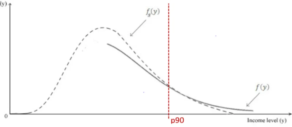
Since this OBE series is the only known survey of the full distribution of income prior to the mid-1940s expansion of comprehensive SOI data, we will use this source to draw some inferences about the shape of the distribution. Specifically, we use the SOI data above the 90th percentile, and the OBE data below the 90th percentile, and harmonize the estimates at this juncture. (Figure
8illustrates.)
We rescale the bottom 90 percent distribution of the OBE distribution according to the known average income level (and total income) from SOI statistics and the national accounts (discussed above), so that the OBE bottom
16If income components and income concepts that change over time, by bracket, this highlights one significant part of the appeal of creating a distributional national accounts measure—such that 100 percent of national income is allocated according to its distribution, regardless of whether it accrues to households as salaries, capital gains, benefits, or other forms of income.
17A few scholars have examined state-level income distributions for the era, a possibility we will return to in discussing further research below.
Figure 8: Harmonizing survey data with tax data. Adapted from Morgan (2018).
90 average and levels match that of the SOI bottom 90. Then we reweight the OBE distribution to accommodate missing tax units, such that family units of the OBE distribution match the tax units of the SOI distribution, with an imputed propensity of joint vs. single filers to seamlessly fit our calculation of a series for equal-split adults. We can only assume that the number of tax units per household is constant over the income distribution from zero to the 90th percentile, and that the propensity to file jointly among OBE households would be that of the SOI population average (making no distinction for tax bracket). Since we have observed from SOI that the majority of income among below-90th percentile income earners comes from wages and salaries, we can repeat the above exercise among the OBE below-90th percentile distribution to move from overall income to wage income. That is, we rescale the OBE income averages according to the known averages of the bottom-90 wage distribution, and we reweight the distribution up to the 90th percentile according to the known population of wage earners.
After these adjustments and the above method of interpolation, we now have estimates for 1929, 1935-36,18 1941, and 1944 that cover the whole population,
for overall income and for wage income, for both tax units and equal-split adults. First, it is important to show that these estimates agree with the benchmark series on top shares. In Figure9we compare these on a tax-unit basis, which is the only comparison available, as previous estimates could not examine equal-split adults.
18As the Goldsmith-OBE dataset is averaged for calendar years 1935-36, we have done the same with the SOI administrative tax records for those years.
Figure 9: Top 10% share of total fiscal income, tax units, 1925-45: Goldsmith-OBE pre-World War II interpolations compared to Piketty-Saez (2003) bench-mark estimates.
Indeed, the data from Selma Goldsmith and the US Commerce Department OBE do match Piketty-Saez (2003) and PSZ (2018) on the top 10% shares of fiscal income, which should not be surprising because we are using SOI data on top 10% shares to harmonize the OBE data. Estimates from the Goldsmith-OBE series are by necessity very rough, given the limitations of the source material, but at the same time they appear to be in the appropriate range to scrutinize further their depth and substance. We have also tested the fidelity of Goldsmith-OBE estimates in 1946, 1955 and 1962, to ensure the similarity with Piketty-Saez (2003), Piketty-Saez-Zucman (2018) and our own estimates. These results are
shown in Appendix 4.
These pre-1945 results can tie seamlessly together with our annual estimates of post-1945 income and wage inequality for the full distribution of equal-split adults. Furthermore, for the pre-1945 years we observe top 10% shares every year, so we can extrapolate shares within the bottom 90% in years for which we do not have survey data, by way of a simple ratio. That is, we take the ratio of distributions within the bottom 90%, to the top 10%, in years for which we do have data, and extend these backward for the bottom 90% in years for which we only have top 10% data.
In this way we show tabulations for bottom 90 percentiles, and a representa-tion of their income distriburepresenta-tion, for several years even before the comprehensive SOI data series began in the 1940s. For the post-war years, we have much more solid evidence from the entire population of tax filers. In all cases, we now can draw inferences on the entire adult population, as well, and not only the tax
units. We can now look inside the bottom 90th percentiles of fiscal and wage income distributions for all years 1913-75.19
From fiscal income to pre-tax national income
Once we have a reliable estimate of fiscal income distribution, it is only a small step to infer the distribution of national income. We do so here on a pre-tax basis, i.e., before the redistributive actions of the tax-and-transfer system (but including pension contributions and receipts among pre-tax income flows).
Specifically, our procedure to move from fiscal income to pre-tax national income is neatly summarized in a recent technical note from Piketty, Saez and Zucman (2019), and we make the following assumptions: (1) Non-fiscal labor income is distributed like fiscal labor income; (2) non-fiscal capital income from pensions is distributed like fiscal labor income; and (3) non-fiscal capital income (from all other sources) is distributed like fiscal capital income.20 The
authors show that this method produces a reliable estimate of pre-tax national income distribution to a first-order approximation, even without the more complex calculations that are feasible with their microdata after 1962 (ibid.). Therefore, even despite the aforementioned limitations in the available data and the associated caveats, we can be confident that our fiscal income estimates equally allow an estimation of pre-tax national income.
We are able to move from fiscal income to pre-tax income, then, because we know the components of fiscal and pre-tax income. That is, we know from which sources tax units earned their income–so we have an estimate of labor (and capital) income within the share of income that is reported to the SOI. Taking the difference of this fiscal labor (capital) income from the total amount of labor (capital) income in the economy as a whole—an amount which can be calculated from national accounts21—we distribute the residual non-fiscal labor
(capital) income according to the principles outlined above.
From this basis and the procedures above, we estimate the full distribution of national income (and its components) for the years 1913-62. While the pre-tax national income estimates are interesting in their own right (see Figure3 above) and perhaps deserve further discussion, the main focus of this paper has been the treatment of fiscal and wage income distributions–which, of course, comprise the majority of earnings among the lower 90 percent of the income distribution.
19Further research could extend these results from SOI raw tabulated data even into the 21st century, although we show below that this method already matches closely with the Piketty-Saez-Zucman microdata estimates for the period of overlap from 1962-75. Micro-data files are available from 1962.
20We also assume zero or negligible re-ranking from the differences between fiscal and non-fiscal income distributions.
21These macroeconomic components are reported in the appendix materials to Piketty, Saez, Zucman (2018)
Therefore, the fiscal and wage income distributions are the backbone of our analysis, in both the statistical procedure above and in the economic reality it reflects (in both the data- and the income-generating processes, one might say). For this reason, although our data and new results do extend more broadly to cover all of national income and its component parts, for the full income distribution from 1913-62, we will strictly concentrate our discussion here on midcentury fiscal and wage inequality patterns for poor and middle-class households.
On this note, we turn to the main results.
3
Results
Income inequality, 1913-75
Using the method discussed above to harmonize survey data with administrative tax tabulations, we were able to extend estimates of the lower 90% income distribution to the pre-World War II period. That is, we complement the Piketty-Saez (2003) and PSZ (2018) benchmark series on top shares with data even for the bottom 50% and middle 40% of earners.
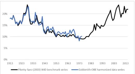
We have harmonized the Goldsmith-OBE series with the SOI tax data to create a unified long-run series on income distribution that includes pre-1945 fiscal income shares. Compared to the Piketty-Saez (2003), this new series is robust and comparable in most years. (See Figure10.)
These estimates also match closely at the level of top 1% shares (Figure 11). In their time periods of overlap, these new estimates are similar to those in Piketty-Saez (2003) and Piketty-Saez-Zucman (2018), and match closely. Of course, the advantage of using this new dataset for the pre-war years goes beyond just the appeal of a replication study with more detailed data.
From the harmonized Goldsmith data series, we can now estimate the lower 90th percentile income distribution, and for equal-split adults, as well. Therefore, we present the new data series, first for tax units (Figures12and13) and then for equal-split adults (Figures14and15).
Immediately apparent is the dramatic rise of top incomes in the pre-World War II era, and its fall in the wartime and post-war era. These tectonic shifts predominantly affected the middle class households (tax units) in the 50th to 90th percentile distributions. Of course, incomes of the lower 50% of households fell sharply during the Great Depression and rose even more notably during and after the war, but the magnitude of these changes was not as large as that of the
Figure 10: Top 10% share of total fiscal income, tax units, 1913-75: Harmo-nized Goldsmith-OBE pre-war interpolations and raw SOI data post-war, compared to Piketty-Saez (2003) benchmark estimates.
Figure 11: Top 1% share of total fiscal income, tax units, 1913-75: Harmo-nized Goldsmith-OBE pre-war interpolations and raw SOI data post-war, compared to Piketty-Saez (2003) benchmark estimates.
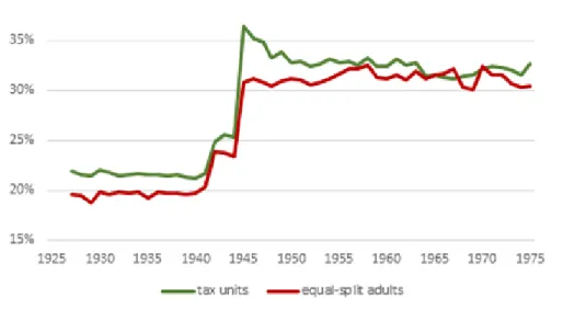
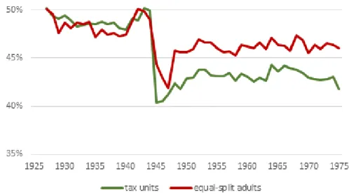
Figure 12: Middle 40% share of total fiscal income, tax units, 1913-75: Goldsmith-OBE pre-World War II interpolations harmonized with SOI tax data.
Figure 13: Bottom 50% share of total fiscal income, tax units, 1913-75: Goldsmith-OBE pre-World War II interpolations harmonized with SOI tax data.