Static analysis of concurrent programs based on behavioral type systems

(1)

HAL Id: tel-01660749

https://hal.inria.fr/tel-01660749

Submitted on 11 Dec 2017

HAL is a multi-disciplinary open access

archive for the deposit and dissemination of sci-entific research documents, whether they are pub-lished or not. The documents may come from teaching and research institutions in France or abroad, or from public or private research centers.

L’archive ouverte pluridisciplinaire HAL, est destinée au dépôt et à la diffusion de documents scientifiques de niveau recherche, publiés ou non, émanant des établissements d’enseignement et de recherche français ou étrangers, des laboratoires publics ou privés.

behavioral type systems

Abel Celestrín

To cite this version:

Abel Celestrín. Static analysis of concurrent programs based on behavioral type systems. Program-ming Languages [cs.PL]. University of Bologna, 2017. English. �tel-01660749�

(2)

DOTTORATO DI RICERCA IN INFORMATICA

Ciclo: XXIX

Settore Concorsuale di A↵erenza: 01/B1 Settore Scientifico Disciplinare: INF/01

Static analysis of concurrent programs

based on behavioral type systems

Presentata da: Abel Garc´ıa Celestr´ın

Coordinatore Dottorato: Paolo Ciaccia

Relatore: Cosimo Laneve

Esame finale anno 2017

(3)

(4)

Abstract

The strength of program static analysis techniques lies on its ability to de-tect faulty behaviors prior to the execution. This ability requires that the analysis process foresees any possible runtime scenario. A task which is even more complex in the case of concurrent programs, because of the number of alternatives introduced by the usual nondeterminism. In this particular case, some of the most common faulty behaviors are those about erroneous usage of resources, presence of deadlocks and data race conflicts.

Behavioral type systems for programming languages provide a strong mechanism for reasoning on programs actions at static time. In this the-sis we discuss two static analythe-sis techniques based on this approach. The first one, targets the resource usage in an ad-hoc language with full-fledged operations for acquiring and releasing virtual machines. The second one, targets the deadlock analysis of Java programs.

In both cases we provide a formal proof of correctness, along with pro-totype implementations that allow practically to test the feasibility of these solutions. These prototypes have also allowed assessing these techniques against others existing in the literature obtaining very encouraging results.

(5)

Acknowledgements

During your life as Ph.D. Student several people crosses paths with you, in such a moment of your life you get to appreciate even the slightest act of support. To all of them I want to express my appreciation and gratefulness. That said, there are some persons that in one way or another become special by living this experience by your side.

A very deep gratitude goes to my advisor Prof. Cosimo Laneve, I will always take with me the rewarding discussions, and the enormous support in the process of writing and describing scientific results. Of course, I will not forget either the passion for the science, and the stylish approach in presentations (which I have, secretly, tried to imitate a lot).

I also want to thank Elena Giachino for being not only a colleague but also a friend since day one, with whom I have shared amazing moments both professionally and personally speaking.

I want to thank my Ph.D. colleagues: Valeria, Stefano, Francesco, Vin-cenzo and VinVin-cenzo ”the master”, and Giacomo, for contributing to create a really nice work environment, and for bringing a nice warm atmosphere to our cold basement. A special gratitude goes to Saverio Giallorenzo for being always two steps forward but showing the rest of us the right way ahead.

I feel very grateful as well to all the people in the Envisage Team. In particular, to Reiner Hanle who invited me to Germany and to his amazing team that make me feel at home there. And to Einar Broch and Elvira Albert who kindly accepted being part of the reviewing committee of this thesis.

Finally, I want to thank Yisleidy Linares (my Yiyi) who is my partner in life but also happens to be a Ph.D. colleague. I don’t know how these three years would have resulted without having here supporting me every single day.

(6)

Chapter 1 Introduction

In this Chapter we present a general overview of the concepts and problems treated in this thesis. We start with a brief description of the purpose of program static analysis, and in particular, the behavioral type system based approach. Then, we concisely describe the two program verification problems that are solved by the static techniques presented in this work. Finally, we conclude with the main goals of this thesis and the structure of this document.

1.1 Static analysis

There are two big well-defined groups of approaches for program analysis: static analysis techniques and runtime analysis techniques. In addition, there are as well hybrid techniques that combine the previous two.

The main characteristic of static analysis techniques is that programs are verified without actually being executed. Usually such analyses are per-formed on the source code or, in other cases, on some form of the object code (the intermediate language generated by some compilers like JVML in the case of the Java virtual machine). The term static analysis is, in general, applied to a verification performed in an automatic way. There are human-aided static analysis tools as well, but these are usually referred in the literature as program understanding, program comprehension, or code review.

The vast majority of the existing programming languages use some sort of static analysis for detecting potential errors prior to the execution time. The simplest examples are perhaps strong-typed languages, that define a type system that is checked at compiling time for ensuring type safety.

However, other kind of properties (i.e. resource usage upper bounds, deadlock freedom, program termination and data race conflicts) may be much more difficult to verify.

(11)

The advantage of the static analysis tools is the possibility to reason about the whole set of possible program executions. Theoretically, such checking ensures a certain quality before the software deployment stage. In general, the static analysis is as complex as the properties targeted by the verification. Logically, when these properties become very complex, the main drawbacks of these approaches appear.

The main issues with static analysis techniques is that analyzing all possi-ble program executions takes a considerapossi-ble amount of time. It is important to consider that since static techniques take place during compilation time they are not as time sensitive as dynamic analysis techniques that take place during the program runtime. Still, even for not very big programs, analyzing the whole set of possible executions may lead to an exponential unmanage-able problem. Therefore, for non-trivial programs, some level of abstraction is needed. Abstraction allows to scale the large set of possible program runs into a smaller (analyzable) model. Implicitly, this produces a common trade-o↵ in static analysis techniques between precision and abstraction.

Formal methods. Program verification has been targeted by the Com-puter Science community since the very beginning. Perhaps one of the very first problems in this sense was Alan Turing’s halting problem [57]. To this aim, several formal methods have been developed oriented to the analysis of computer programs. A static analysis technique may be purely based on one of these techniques, or on a combination of them. The following list briefly summarizes some of the most used formal methodologies:

Abstract interpretation: A technique based on the interpretation of an abstraction of the language semantics. This technique often uses over-approximations of the underlying program model in order to con-siderably reduce the set of possible program executions.

Model checking: This technique is built around the representation of a program by a finite set of states. These states are then analyzed sep-arately and the resulting conclusions are combined to draw the overall verification of the program.

Symbolic execution: This technique tries to fill the gap between the static and dynamic analysis. The main idea is to group all the possible inputs of the program into sets that will produce similar behaviors. Afterwards, a symbolic representation of each set of inputs is evaluated by a symbolic interpreter. The final conclusions are drawn from the results of this symbolic execution.

(12)

Dataflow analysis: This is a fix-point based technique. Programs are represented by a control flow graph that corresponds to the source code. The states at each node of the program are then calculated repeatedly until a stable state is reached. Then, the verification is performed on each one of the control flow graph nodes.

1.2 Behavioral type systems based analysis

Behavioral type systems [11] provide a strong mechanism for reasoning on a program possible execution. With respect to standard type systems, the behavioral ones usually enrich standard types by adding some dynamic in-formation of the e↵ects of each expression.

Generic approach

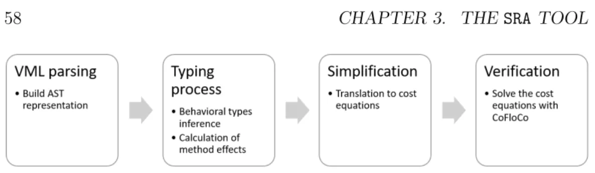
The overall approach can be divided in four stages: i Parsing of the pro-gram, ii Typing process, iii Simplification of the program and iv Veri-fication of the program.

The first step is usually performed after traditional static checks, thus the program is considered syntactically correct and with no obvious semantic errors. The main goal of this process is to obtain a representation of the program that is more suitable for the upcoming processes than the textual representation.

During the typing process the program behavioral type is obtained. This process can be fully automatic, partially automatic or manual. The typing process might not succeed, in that case the program could not be analyzed. After a behavioral type is obtained, it is derived into an abstract simpli-fied representation of the program. This abstraction drops features that are unrelated to the targeted analysis and focuses on those that are relevant. For example, in deadlock analysis, the abstraction may be an object dependency graph, for resource analysis it may be a set of cost equations.

Finally, the targeted properties are verified over the abstracted program. The verification process is only tied to the abstract program representation easing the use of third-party, and possibly more general, analyzers.

Advantages

The main advantage of this approach is its modularity. The type system is in general bounded to the language targeted by the analysis. The final verification is, in turn, tied to the abstract representation of the program.

(13)

This makes possible to apply the same analysis to di↵erent programming languages by having proper typing mechanisms producing the same kind of abstract representation.

This idea is illustrated in Figure 1.1. The figure corresponds to the dead-lock analysis scheme for three di↵erent programming languages Java, Scala and ABS1_{. All three languages share the verification stage, since all three share}

the same simplified representation. However, there are two typing processes, one for Java and Scala, and the other for ABS. The first two languages can use the same inference mechanism since both of them are compiled to Java bytecode.

Figure 1.1: General approach of a behavioral type system based analysis

Another rather important advantage is that one can reason on the cor-rectness of the analysis also in a modular way. For example, one can focus on two aspects separately: the typing and the abstraction, and the analy-sis. In the case of the typing process and its abstract representation, the correctness is usually proved by means of a subject reduction technique [24]. The correctness for the analysis will depend on the analysis technique. For example, in the case of the work described in Part I the correctness of the verification relies on the third party cost equation solver. In the case of the work described in Part II the analysis is based on a formally demonstrated decision algorithm.

(14)

1.3 Problems tackled in this work

This work presents the theoretical basis and the prototype implementation of two static analysis tools based on behavioral type systems. The two problems targeted by these tools are the analysis of resource usage upper-bounds and the deadlock analysis. In both cases, the targeted language is an object-oriented language that allows concurrency operations.

The description of both tools is presented in the order they were con-ceived. This is an important remark, because the experience obtained in the development of the first tool has been key in the conception of the second one. In practice, it can be appreciated that the second of these tools presents a much deeper level of complexity. Also, in this second tool the result is more palpable since it can be applied to real world programming languages.

The analysis of virtual machines usage. In the first problem we analyze a domain specific language called vml. This is a rather simplistic language but expressive enough to allow the dynamic acquisition (creation) and releas-ing (deletion) of objects representreleas-ing virtual machines. In this language, the operations on virtual machines can occur in parallel, and more over, virtual machine objects can run tasks that may, in turn, operate on other virtual machines. This scenario is inspired on the elastic features of the Cloud Com-puting environments. The purpose of the analysis of this language is to make an (over) estimation of the maximum number of virtual machines that may coexist during the program execution.

The resource analysis problem itself has received lots of attention from the scientific community. However, very few approaches target languages in which are both present, the concurrency feature and the explicit resource removal operation. Moreover, to the best of our knowledge, there are not previous works targeting the static analysis of code exploiting the Cloud elasticity features.

The analysis of deadlocks in Java bytecode. There have been several works targeting the analysis of deadlocks in the Java language and its byte code (JVML). The existing techniques, however, target either a very reduced subset of the language or take little to none consideration about the sound-ness of their approach. An interesting remark, is also the fact, that to the best of our knowledge none of the existing analyzers reports the analysis of Scala programs, a language that is also compiled into JVML.

(15)

1.4 Aim, objectives, and contribution of this

work

The main goal of this thesis is to present the strength of the behavioral type system based approach for the static analysis in concurrent programs. To accomplish such purpose, we focus on two program verification problems of high relevance and with application in the newest developments in the Computer Science world.

It is also part of the aim of this work to produce competitive solutions to these problems at the level of other state of the art solutions. We also expect these solutions to be fully automatic and capable to perform with very little human interaction. This is a key feature for the purpose of analyzing non-trivial programs

1.4.1 Objectives

The main objective of this thesis is to provide valid tools for the analysis of the problems discussed in Section 1.3. Technically, the process of building such tools, with the approach followed in this work, involves the following partial objectives:

• Definition of the behavioral type systems: To design the static semantic rules that define the type systems for both of the problems tackled in this work.

• Design and implementation of automatic behavioral type in-ference: To implement a fully automatic mechanism for the inference of program types, according to the behavioral type systems designed and the targeted languages.

• Proofs of correctness of the behavioral type systems: To demon-strate the correctness of the behavioral type systems in characterizing the underlying programs and producing correct program abstractions without losing key information for the analysis.

• Design and implementation of the analysis of the behavioral type systems: To provide an automatic mechanism for drawing con-clusions from the abstractions produced during the typing process. • Comparison of the result of the proposed tools with existing

similar ones: To demonstrate the e↵ectiveness of the resulting tools by testing them against other related approaches.

(16)

1.4.2 Contribution

Two main contributions can be derived from the results of this work:

i the approach for the static analysis of resource utilization in a concur-rent and object oriented language with explicit resource release opera-tions.

ii the approach for the static analysis of deadlocks in Java bytecode.

Each of these solutions presents a custom and complex behavioral type system. The instrumentation of these type systems as well as the proof of correctness behind them are also a remarkable part of the results obtained in this work.

The design of these solutions cover issues that are typical in the static analysis of programs. The ways in which these issues are resolved constitute also relevant contributions of this work.

Finally, this work also provides a prototype implementation of the two solutions described. These prototypes constitute a simple way to interact with the results of these approaches making easy to compare it with previous and future equivalent techniques.

1.5 Document contents

The current document intends to provide an overall vision of the static analy-sis techniques based on behavioral type systems, and to present two successful applications of this approach. Following this introduction, the document is divided in two parts of two chapters each:

Part I: The static resource analysis problem

This part is dedicated to the analysis of resources in a concurrent object oriented language. The content is divided in two chapters. Chapter 2: Machine usage upper bounds in vml, describes a vari-ation of the static resource analysis problem applied to the Cloud Computing scenario. In particular, this problem focuses in the detection of upper bounds for the number of virtual machines nec-essary to execute a program in this environment. In this chapter, we describe a custom language: vml, which allows modeling the dynamic creation and release operations of the Cloud’s elasticity feature. We then discuss a behavioral type system for abstract-ing virtual machine usage on these programs, and the subsequent

(17)

analysis of these types. This chapter concludes with the proof of correctness of the overall process.

Chapter 3: The SRA tool, describes a resource analysis tool based on the theory presented in Chapter 2. We discuss the main imple-mentation details of this tool, specially the type inference process and the integration with an external cost equations solver. We present illustrative examples of the technique, and we also review the related literature and compare the tool and its technique with some of the existing approaches.

Part II: The deadlock analysis problem

This part is devoted to the deadlock analysis problem in Java programs. The content is divided in two chapters.

Chapter 4: Deadlock detection in JVML, describes the static deadlock analysis problem in Java programs. In this chapter, we present a behavioral type system for abstracting dependen-cies in JVMLd, a subset of the Java bytecode. We also present the algorithm for reasoning on the presence of circularities in the program dependencies. The chapter concludes with the extension of the behavioral type system to the full set of Java features and the proof of correctness of the overall approach.

Chapter 5: The JaDA tool, describes the Java deadlock analysis tool. We discuss the type inference process and the implementa-tion of the circularities detecimplementa-tion algorithm. In this chapter, we also review the related literature and compare the tool and its technique with some of the existing approaches including a com-mercial grade tool. We conclude with the description of the JaDA tool deliverables.

This document concludes with Chapter 6, where we present the main contributions of this thesis and describe some of the future possible lines of research that can be derived from it.

(18)

Part I

The static resource analysis

problem

(19)

(20)

Chapter 2 Machine usage upper bounds in

vml

Summary

We propose a static analysis technique that computes upper bounds of virtual machines usage in a concurrent language with explicit acquire and release operations over this kind of objects. In our language, the creation and re-lease operations can occur in separated and possibly concurrent contexts (by passing virtual machine objects as arguments of invocations). Moreover, the objects representing virtual machines are active, that may be asynchronously hosting operations with side e↵ects on the overall resource utilization. Our technique is modular and consists of (i) a type system associating programs with behavioral types that record relevant information for resource usage (creations, releases, and concurrent operations), (ii ) a translation function that takes behavioral types and returns cost equations, and (iii) the integra-tion with an automatic o↵-the-shelf solver for the cost equaintegra-tions.

2.1 Introduction

An accurate assessment of the resource usage in a computer program could reduce, for example, energy consumption and allocation costs. Two criteria that are even more important today, in modern architectures like mobile devices or Cloud Computing, where resources, such as virtual machines, have hourly or monthly rates.

While it is relatively easy to manually estimate worst-case costs for sim-ple code examsim-ples, extrapolating this information for fully real-life comsim-plex programs could be cumbersome and highly error-sensitive. The first attempt

(21)

about the analysis of resource usage dates back to Wegbreit’s pioneering work in 1975 [58], which develops a technique for deriving closed-form ex-pressions out of programs. The evaluation of these exex-pressions would return upper-bound costs that are parametrized by programs’ inputs.

Wegbreit’s contribution has two limitations: it addresses a simple func-tional language and it does not formalize the connection between the lan-guage and the closed-form expressions. A number of techniques have been developed afterwards to cope with more expressive languages (see [6, 20]) and to make the connection between programs and closed-form expressions precise (see [23, 41]). A more detailed discussion of the related work in the literature is presented in Section 2.8.

The existing cost analysis techniques vary also from the point of view of the resource targeted. The most common targets are probably the memory related resources like the heap space, and the number of steps in the pro-gram execution. However, some of the existing techniques also give certain abstraction on the type of the resource analyzed, by allowing code annota-tions with cost related expressions. Some attempts have even considered the analysis of the time necessary for the program execution [33].

This work targets the analysis of the usage of virtual machines repre-sented by first order objects in a custom domain specific language called vml. The latter is a concurrent object-oriented language that includes explicit ac-quire and release operations on virtual machines object. These operations can occur in separated and possibly concurrent contexts (by passing virtual machine objects as arguments of invocations).

Our technique is modular and consists of (i) a type system associating programs with behavioral types that record relevant information for resource usage (creations, releases, and concurrent operations), (ii) a translation func-tion that takes behavioral types and returns cost equafunc-tions, and (iii) the integration with an automatic o↵-the-shelf solver for the cost equations.

To the best of our knowledge, current cost analysis techniques address (concurrent) languages where resource usage is always cumulative. We have found that only one of the existing techniques considers the scenario where both concurrent and resource removal operations are possible. That is the case of [8], however, our problem settings di↵er from these in two main aspects: i) the resources targeted by our technique are program objects that may carry, concurrently, operations that acquire and release other resources; and ii) in our case it is possible to have the acquire and release operations of a resource happening in di↵erent contexts by passing the objects as arguments of other possibly asynchronous method invocations.

(22)

Chapter contents

This Chapter starts by describing, in Section 2.2, the so called Cloud Com-puting elasticity concept that constitutes the inspiration of this work. In Section 2.3, we present vml: a simplified concurrent object-oriented language featuring virtual machine (VM) objects. In Section 2.4 we discuss some tech-nical limitations that simplify, from the practical point of view, the analysis of vml programs. Section 2.5 and 2.6 present the definition of a behavioral type system for vml programs and its further analysis for estimating VM usage upper bounds. We then discuss, in Section 2.7, the correctness of this approach, supported by the formal proof of the soundness of the type system and the corresponding analysis. In Section 2.8 we review some of the main contributions in the literature related to the resource analysis problem. We conclude with the main remarks about this approach.

2.2 Motivation and Problem Statement

Cloud Computing introduces the concept of elasticity, whose main feature is the possibility for the resources, namely virtual machines (VM), to scale according to the software needs. There are two kinds of scaling, vertical and horizontal. Vertical Scaling means changing the deployed VM, adding more memory or disk space or using a more powerful processor, this kind of elasticity is, in general, associated to a disruptive workflow that stops the software execution and restarts it after the changes.

On the other hand, Horizontal Scaling is when the underlying number of VMs changes to fulfill the demand, this kind of scaling is a seamless process for the final user since it does not a↵ect the availability of a service. Hori-zontal Scaling is the suggested scaling method by main Cloud providers like Amazon, Google and Microsoft Azure. This is appreciated in their pricing models that allow hiring, on demand, instances which are payed for the time they are in use; and also in their APIs that include instructions for requesting and releasing these VM instances on the fly.

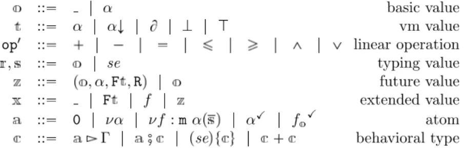
In contrast to the elasticity concept, Cloud providers also give to the user the possibility to reserve a number of VM instances for a fixed period of time. This approach is used often by clients that migrate their existing solutions from private data centers to the Cloud. The main problem of this approach is the overcapacity or under-capacity of the allocated resources. The reserved VMs may spend important part of the time in an idle status, or the reserved VMs may be not enough to fulfill the demand. The table in Figure 2.1 shows some of the pricing possibilities given by the main Cloud providers. Notice

(23)

that the on demand price is a bit higher than the reserved alternative. However, the on demand model is more convenient when reserved machines may be idle more than the 40% of the time.

Figure 2.1: Some pricing options of main Cloud Providers, January 2016

Cloud computing elasticity APIs features acquire and release operations for the management of On Demand VMs (see for instance the Amazon Elastic Compute Cloud [50] or the Docker Fiware) that can be invoked dynamically from running code. The release operation happens to be a very powerful pro-gramming artifact, allowing to downscale a program’s resource demand. It is worth noticing that, without a full release operation, the cost of a concur-rent program may be modeled by aggregating the sets of operations that can occur in parallel, as in [7]. A full-fledged release operation, however, makes possible to delegate to other methods (possibly concurrent) the release of re-sources by passing them as arguments of invocations. For example, consider the following method

Int double_release(Vm x, Vm y) {

release x;

release y;

return 0 ; }

that takes two machines and simply releases them. The cost of this method will depend on the state of the machines in input:

– it may be -2 when x and y are di↵erent and active;

– it may be -1 when one machine is active and the other is released, or

(24)

– it may be 0 when the two machines have been already released.

In this case, one might over-approximate the cost of double_release to 0. However, this leads to disregard releases and makes the analysis (too) impre-cise. Moreover, consider the case where the machine objects can be hosting processes that either create or release other virtual machines. Ignoring a ma-chine release may imply to assume the process hosted on it is still running, thus executing in parallel with the rest of the environment. This will have a serious impact in the calculation of the usage of these resources.

Problem statement

Lets us consider the following problem:

Given a pool of on demand VM instances and a computer pro-gram that may indistinctly acquire and release these instances, what is the minimum cardinality of the pool that ensures the pro-gram runs without interruptions caused by the lack of available VMs? Assume that a VM can be re-acquired if and only if it has been previously released.

A solution to the previous problem has a direct application for both Cloud Providers and Cloud Costumers. For the former, it represents the possibility to know in advance how many real resources to allocate for an specific service. For the latter, it represents the possibility to pay exactly for the resources that are needed.

2.3 The language vml

The language vml is a future-based concurrent object-oriented language1 _with

explicit acquire and release operations of virtual machines. In future-based languages, function/method invocations are executed asynchronously to the caller and are bound to variables called futures. The caller synchronizes with the callee by using the future variables when the return value is strictly needed. The syntax and the semantics of vml are defined in the following two subsections; the third subsection discusses a number of examples.

2.3.1 Syntax

In vml we distinguish between simple types T , which are either integers Int or virtual machines VM, and future types Fut<T >, which type asynchronous

(25)

invocations. The future argument T is instantiated with the return type of the invoked function. We use F to range over simple and future types. The notation T x denotes any finite sequence of name declarations T x separated by commas. Similarly we write T x ; for a finite sequence of name declaration separated by semicolons.

A vml program is a sequence of method definitions T m T x F y ; s , ranged over M , plus a main body F z ; s . The syntax of statements s, expressions z and pure expressions e of vml is defined by the following grammar:

s :: x z ife s else s returne s ; s releasee statements

z :: e e!m e e

.

get new VM expressions

e :: this se nse pure expressions

A statement s may be either one of the standard operations of an impera-tive language plus the release e operation that disposes the virtual machine e.

An expression z may change the state of the system. In particular, it may be an asynchronous method call e!m e where e is the virtual machine that will execute the call, and e are the arguments of the call. This invoca-tion does not suspend caller’s execuinvoca-tion: when the value computed by the invocation is needed then the caller performs a non blocking get operation, if the value needed by a process is not available then an awaiting process is scheduled and executed. Expressions z also include new VM that creates a new virtual machine. The intended meaning of operations taking place on di↵erent virtual machines is that they may execute in parallel, while opera-tions in the same virtual machine interleave their evaluation (even if in the following operational semantics the parallelism is not explicit).

A (pure) expression e may be the reserved identifier this, a virtual ma-chines identifier or an integer expression. Since our analysis will be paramet-ric with respect to the inputs, we parse integer expressions in a careful way. In particular we split them into size expressions se, which are expressions in Presburger arithmetics [18] (this is a decidable fragment of Peano arith-metics that only contains addition), and non-size expressions nse, which are the other type of expressions. The syntax of size and non-size expressions is the following:

nse :: k x nse nse nse nse and nse non-size expressions

nse or nse nse nse nse nse

nse nse nse nse

se :: ve ve ve se se and se se or se size expressions

ve :: k x ve ve k ve integer size expressions

(26)

We will use the term nse nse as an abbreviation of “ nse nse and nse nse ”, and similarly for se. We notice that (non-size and size) expressions also contain the value err – see below the definition of e l for

the semantics of arithmetics expressions that contain err. In the whole docu-ment, we assume that sequences of declarations T x and method declarations M do not contain duplicate names. We also assume that return statements never have a continuation.

2.3.2 Semantics

The vml semantic is defined as a transition relation between configurations, noted cn and defined below

cn :: ✏ fut f, v vm o, a, p, q invoc o, f, m, v cn cn configurations

p :: l ✏ l s process

q :: ✏ p q q sets of processes

v :: integer constants o f err run-time values

a :: machine states

l :: , x v, maps

Configurations are sets of elements – therefore, we identify configurations that are equal up-to associativity and commutativity – and are denoted by the juxtaposition of the elements cn cn; the empty configuration is denoted by ✏. The transition relation uses two infinite sets of names: VM names, ranged over by o, o , and future names, ranged over by f , f , . The function fresh returns either a fresh VM name or a fresh future name; the context will disambiguate between the two. The elements of configurations are:

– virtual machines vm o, a, p, q where o is a VM name; a is either or depending on whether the machine is alive or dead; p is either

l ✏ , representing a terminated statement, or l s , representing an active process, where l maps each local variable to its value and s is the statement to execute; and q is the set of processes to evaluate.

– future binders fut f, v . When the value v is then the actual value of f has still to be computed.

– method invocation messages invoc o, f, m, v .

Runtime values v are either integers or virtual machines and future names, or , meaning an un-computed value, or an erroneous value err. The

(27)

fol-lowing auxiliary functions are used in the semantic rules (we assume a fixed vmlprogram):

– dom l returns the domain of l.

– l x v is the function such that l x v x v and l x v y l y , when y x.

– e l returns the value of e, possibly retrieving the values of the names

that are stored in l. Regarding boolean operations, as usual, false is represented by 0 and true is represented by a value di↵erent from 0. Arithmetic operations in vml are also defined on the value err: when one of the arguments is err, every arithmetic operation returns err. e l returns the tuple of values of e. When e is a future name, the

function l is the identity. Namely f l f . It is worth noticing

that e l is undefined whenever e contains a name that is not defined

in l.

– bind o, f, m, v x v, destiny f s o _this _{, where T m T x T z; s}

is a method of the program. We observe that, because of bind, the map l in processes l s also binds the special name destiny to a fu-ture value. We also observe that the local names z do not belong to dom x v, destiny f .

The transition relation rules are collected in Figure 2.2. The rules are almost standard, except those about the management of virtual machines and method invocations, which we are going to discuss.

Rule (New-VM) creates a virtual machine and makes it alive. Rules (Release-VM) and (Release-VM-self) dispose a virtual machine by means of the operation release x: this amounts to update its state a to . Once a virtual machine has been released, no operation can be performed anymore by it, except letting the processes on the queue returning err – see rules (Activate), (VM-Err-Return), and (Bind-Mtd-Err).

Rule (Async-Call) defines asynchronous method invocation x e!m e . This rule creates a fresh future name that is assigned to the identifier x. Rule (Bind-Mtd) applies an invocation message by adding to the alive callee vir-tual machine a process corresponding to the called method. In case the callee virtual machine is not live, either (Bind-Mtd-Err) or (Bind-Partial) is applied, which binds err to the future name. Rule (Read-Fut) allows the caller to retrieve the value returned by the callee. It is worth noticing that the semantic of get is di↵erent from that of ABS [46] or of [35] because it is not blocking with respect to other processes waiting to be executed on the

(28)

(Assign) v e l vm o, , l x e; s , q vm o, , l x v s , q (Read-Fut) f e l v vm o, , l x e

.

get; s , q fut f, v vm o, , l x v; s , q fut f, v (Async-Call) o e l v e l f fresh vm o, , l x e!m e ; s , q vm o, , l x f ; s , q invoc o , f, m, v (Bind-Mtd) l s bind o, f, m, v vm o, , p, q invoc o, f, m, v vm o, , p, q l s fut f, (Cond-True) e l 0 e l err vm o, , l if e then s1 else s2 ; s , q vm o, , l s1; s , q (Cond-False) e l 0 or e l err vm o, , l if e then s1 else s2 ; s , q vm o, , l s2; s , q (New-VM) o fresh VM vm o, , l x new VM ; s , q vm o, , l x o ; s , q vm o , , ? " , ? (Release-VM) o e l o o vm o, , l release e; s , q vm o , a , p , q vm o, , l s , q vm o , , p , q (Release-VM-self) o e l vm o, , l release e; s , q vm o, , l s , q (Return) v e l f l destiny vm o, , l return e , q fut f, vm o, , l " , q fut f, v (VM-Err-Return) f l destiny vm o, , l s , q fut f, vm o, , l; " , q fut f, err (Activate) vm o, a, l " , q l s vm o, a, l s , q (Activate-Get) f e l vm o, , l x e

.

get; s , q l s fut f, vm o, , l s , q l x e

.

get; s fut f, (Bind-Mtd-Err) vm o, , p, q invoc o, f, m, v vm o, , p, q fut f, err (Bind-Partial) invoc err, f, m, v fut f, err (Context) cn cn cn cn cn cn Figure 2.2: Semantics of vml.

same machine, see rule (Activate-Get). In fact, deadlock freedom is out of the scope of this contribution; in any case we refer to [35] for an algorithm (and a prototype) verifying deadlock freedom in ABS.

The initial configuration of a vml program with main body F x ; s is vm start, , destiny fstart s start this ,?

where start is a special VM name and fstart is a fresh future name. As usual,

let be the reflexive and transitive closure of and represents (part of) computations.

Problem statement reformulation

After discussing the semantics of vml we can now reformulate the Problem Statement from Section 2.2 in a more formal way. We start by defining the concept of alive machines:

(29)

Definition 3.1 (Alive machines). Given a configuration cn, a term

vm o, , p, q cn is called alive machine in cn. Let alive cn be the number of di↵erent alive machines in cn.

At this point we can rewrite the objective of this work as:

to define a technique such that, given a configuration cn, it re-turns a n satisfying, for every cn cn , alive cn n (n is an upper bound to the alive machines in computations rooted at cn).

2.3.3 Examples

We now proceed to illustrate vml by discussing few examples and, for every example, we also examine the output we expect from our cost analysis. We begin with two methods computing the factorial function:

Int fact(Int n){

Fut<Int> x ; Int m ;

if (n==0) { return 1 ; }

else { x = this!fact(n-1) ; m = x.get ;

return m*n ; }

}

Int costly_fact(Int n){

Fut<Int> x ; Int m ; VM z ;

if (n==0) { return 1 ; } else { z = new VM(); x = z!costly_fact(n-1) ; m = x.get ; release z; return m*n; } }

The method fact is the standard definition of factorial with the recursive invocation fact(n-1) always performed on the same machine. That is, the computation of fact(n) only requires one virtual machine. On the contrary, the method costly_fact performs the recursive invocation on a new virtual machine z. The caller waits for its result, let it be m, then it releases z and delivers the value m*n. Since every virtual machine creation occurs before any release operation, costly_fact will create as many virtual machines as the argument n. That is, if the available resources are k virtual machines, then costly_fact can compute factorials up-to k.

The analysis of costly_fact has been easy because the release oper-ation is applied to a locally created virtual machine. Yet, in vml, release can be also applied to method arguments and the presence of this feature in concurrent codes is a major source of difficulties for the analysis. A paradig-matic example is the double_release method discussed in Section 2.2 that may have either a cost of -2 or of -1 or of 0.

It is worth observing that, while over-approximations (e.g not count-ing releases) return (too) imprecise costs, under-approximations may return

(30)

wrong costs. For example, the following method creates two virtual ma-chines and releases the second one with this!double_release(x,x) before the recursive invocation.

Int fake_method(Int n) {

if (n=0) return 0 ;

else { VM x, y ; Fut<Int> f, g; Int u, v; x = new VM() ; y = new VM() ;

f = this!double_release(x,x) ; u = f.get ; g = this!fake_method(n-1) ; v = g.get ;

return 0 ; } }

The cost of fake_method(n) should be n. However this is not the case if double_release is under-approximated with cost -2: In such case, one would wrongly derive a cost 0 of fake_method(n). In Section 3.4 we con-sider an erroneous fake_method that increases the argument of the recursive invocation (instead of decreasing it) and discuss the corresponding cost equa-tions returned by our technique. We notice that, in this case, the amount of virtual machines used by the erroneous method is infinite. The aim of the following sections is to present a technique for determining the cost of method invocations. Such a technique has to be sensible to the identity, and to the state of method’s arguments before and after the invocation.

2.4 Determinacy of method’s arguments release

Our cost analysis of virtual machines uses abstract descriptions that carry informations about concurrent method invocations and about creations and removals of virtual machines. In order to ease the compositional reasonings, method’s abstract descriptions also define the arguments the method releases upon termination, called method’s e↵ects. In this contribution we stick to method descriptions that are as simple as possible, namely we assume that method’s e↵ects are sets. In turn, this requires methods’ behaviours to be de-terministic with respect to method’s e↵ects and, to enforce this determinacy, we define the following simplification properties.

The following simplifications allow us to focus on the relevant problems of the resource analysis of vml. It is possible to drop most of the simplifications by extending the approach presented in this work using almost standard so-lutions (for instance, with guarded or nondeterministic e↵ects, see below). However these solutions would entangle a lot the technicalities of this pre-sentation, making more difficult its reading and comprehension.

Simplification 1: the branches in a method body always release the same set of method’s arguments. For example, methods like

(31)

Int foo1(VM x, Int n) {

if (n = 0) return 0 ;

else { release x ; return 0; } }

does not follow this simplification because the then-branch does not release anything while the else-branch releases the argument x.

To analyze such program, one would just have to extend the presented approach with guarded e↵ects, i.e., mapping from execution branches to e↵ects, which can precisely identify the e↵ects of each execution branch of the method.

Simplification 2: method invocations are always synchronized within caller’s body. This implies that method’s e↵ects occur upon method termina-tion. For example, in

Int foo2(VM x, VM y) {

this!double_release(x,y) ; return 0 ; }

the method’s e↵ects of foo2 is not deteministic because double_release might still be running after foo2 termination. This means that the ter-mination of foo2 has no impact on the terter-mination of double_release. Therefore, the e↵ect of foo2 is empty – the caller cannot assume that x and y have been released upon synchronizing with foo2. Overall, this simplification supports a more precise analysis. In order to drop this restriction is necessary to add the unsynchronized invocations to the e↵ects of the method. This idea is explained in [35] and also in Section 4.6 The underlying intuition is to pass the e↵ects of unsyn-chronized invocations to the context, and to consider context e↵ects along with the local e↵ects of each method during the analysis phase.

Simplification 3: machines executing methods with nonempty e↵ects must be alive. (This includes the carrier machine, e.g. method bodies cannot release the this machine.) At static time “alive” means that the ma-chine is either the caller or has been locally created and has not been/is not being released. For example, in foo3

(32)

Int simple_release(VM x) {

release x; return 0; }

Int foo3(VM x) {

VM z ; Fut<Int> f ; Int u ; z = new VM();

f = z!simple_release(x);

release z; u = f.get; return 0; }

Int foo4(VM x, VM y) {

Fut<Int> f ; Int u ; f = x!simple_release(y) ; u = f.get ; return 0 ; }

the machine z is released before the synchronization with the simple_ releasestatement f.get. This means that the disposal of x depends on the scheduler’s choice and, in turn, it is not possible to determine whether foo3 will release x or not. A similar non-determinism arises when the callee of a method releasing arguments is itself an argument. For example, in the above foo4 method, it is not possible to determine whether y is released or not because we have no clue about x, being it an argument of foo4.

To analyze such programs, one would simply need to extend the ap-proach presented in this work with non-deterministic e↵ects.

Simplification 4: if a method returns a machine, the machine must be new. For example, consider the following code:

VM identity(VM x) { return x; } {

VM x ; VM y ; VM z ; Fut<VM> f ; Fut<Int> g ; Int m ; x = new VM() ; y = new VM() ; f = y!identity(x) ; g = this!simple_release(y); z = f.get ; m = g.get ; release z ; }

In this case it is not possible to determine whether the value of z is x or err and, therefore, it is not clear whether the cost of release z is 0 or -1. The non-determinism is caused by identity, which returns the argument that is going to be released by a parallel method.

To analyze programs with such methods, one would simply need to extend the approach presented in this work with non-deterministic ef-fects.

Simplifications 1, 3, and 4 are enforced by the type system in Section 2.5, in particular simplification 1 by rule (T-Method), simplification 3 by rules

(33)

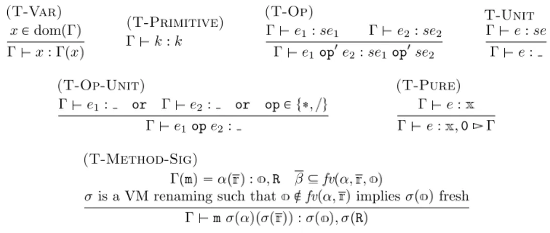
:: ↵ basic value :: ↵ ↵ vm value op :: linear operation , :: se typing value :: , ↵, F , R future value :: F f extended value :: 0 ⌫↵ ⌫f : m ↵ ↵X f X atom :: # se behavioral type

Figure 2.3: Behavioral Types Syntax

(T-Invoke) and (T-Release), and simplification 4 by rules (T-Invoke) and (T-Return).

2.5 The behavioral type system of vml

In this context, Behavioral types are abstract codes highlighting the features of vml programs that are relevant for the resource cost analysis in Section 2.6. These types support compositional reasonings and are associated to programs by means of a set of type system rules that are defined in this section.

The syntax of behavioral types uses vm names ↵, , , , and future names f , f , . Sets of VM names will be ranged over by S, S , R, , and sets of future names will be ranged over by F, F , . We assume that err is a special VM name representing the erroneous machine; therefore VM names will also range over err. The syntactic rules of these types are presented in Figure 2.3.

Behavioral types ⌫↵ and ↵X express creations of virtual machines and their removal, respectively. The type ⌫f : m ↵ defines method invocations and f X defines the corresponding synchronization with the computation of the future f , in this case may be either ↵, which acts like a binder to the name of the returned virtual machine, or if the target of f returns a di↵erent type. The conditional type se behaves like whenever se is true; the type models nondeterminism. We will always shorten the type fX into fX.

In order to have a more precise type of continuations, the leaves of be-havioural types are labelled with environments, ranged over by , , . Environments are maps from method names m to terms ↵ : , R, from names to extended values , from future names to future values, and from VM names to extended values F , which are called vm states in the following. We assume that err ? . These environments occurring in the leaves

(34)

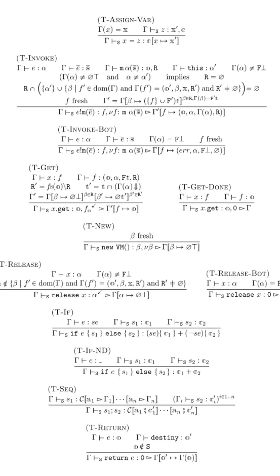
(T-Var) x dom x : x (T-Primitive) k : k (T-Op) e1: se1 e2: se2 e1op e2: se1op se2 T-Unit e : se e : (T-Op-Unit) e1: or e2: or op , e1ope2: (T-Pure) e : e : , 0 (T-Method-Sig) m ↵ : , R fv ↵, ,

is a VM renaming such that fv ↵, implies fresh

m ↵ : , R

Figure 2.4: Typing rules for pure expressions

are only used in the typing proofs and are dropped in the final types (method types and the main statement type).

VM states F are a collection F of future names plus the value of the virtual machines. This F specifies the set of parallel methods that are going to release the virtual machine; defines whether the virtual machine is alive ( ), or it has been already released ( ) or, according to scheduler’s choices, it may be either alive or released ( ). VM values also include terms ↵ and ↵ . The value ↵ is given to the argument machines of methods (they will be instantiated by the invocations – see the cost analysis in Section 2.6), the value ↵ is given to argument values that are returned by methods and can be released by parallel methods (↵ will be also evaluated in the cost analysis). VM values are partially ordered by the relation defined by

↵ ↵ ↵ .

In the following we will use the partial operation returning, whenever it exists, the greatest lower bound between and . For example , but ↵ is not defined.

The type system uses judgments of the following form:

– e : for pure expressions e, f : for future names f , and m↵ : , R for methods.

– S z : , for expressions z, where is the value, is the

behavioral type for z and is the environment with updates of names and future names.

(35)

– S s : , in this case the updated environments are inside the

be-havioural type , in correspondence of every branch of its.

The index S in the judgments for expressions and statements defines the set of method’s arguments – see rule (T-Method) – and is used in the rule (T-Return) in order to constrain that the returned machine, if any, does not belong to method’s arguments (cf. Restriction 4 in Section 2.4).

Since is a function, we use the standard predicates x dom or x dom and the environment update

x y def if y x y otherwise

With an abuse of notation (see rule (T-Return)), we let def (because does not belong to any environment).

We will also use the operation and notation below: – F is defined as follows:

F def

if F ? if F ? and ↵ if F ? and ↵

and, in Section 2.6, we write F1 1, , Fn n for F1 1 , , Fn n

.

– the multihole contexts C defined by the following syntax:

C :: _{# C} C C se C

and, whenever _C 1 1 n n , then x is defined

asC 1 1 x n n x .

The type system for expressions is reported in Figure 2.4. It is worth noticing that this type system is not standard because (size) expressions containing method’s arguments are typed with the expressions themselves. This is crucial in the cost analysis of Section 2.6. It is also worth observing that, by rule (T-Primitive), err : err (while err ? ). This expedient allows us to save one rule when typing method invocations with either erroneous or released carriers (cf. rule (T-Invoke-Bot)).

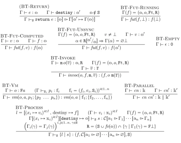
The type system for expressions with side e↵ects and statements is re-ported in Figure 2.5. We discuss rules (T-Invoke), (T-Get), (T-Release), and (T-Return). Rule (T-Invoke) types method invocations e!m e by us-ing a fresh future names. In particular, in the behavioral type ⌫f : m ↵ ,

(36)

the (fresh) future name f is associated to the the method, the VM name of the callee, the arguments and to the returned value. This last value is funda-mental when the invocation returns a new machine because, in this case, the type acts as a binder of . Another important remark is about the value of f in the updated environment. This value contains the returned value, the VM name of the callee and its state, and the set of the arguments that the method is going to remove. The VM state of the callee will be used when the method is synchronized to update the state of the returned object, if any (see rule (T-Get)). It is also important to observe that the environment returned by (T-Invoke) is updated with information about VM names re-leased by the method: every such name will contain f in its state. Let us now discuss the constraints in the second and third lines of the premise of (T-Invoke). As regards the second line, assuming that the callee has not been already released ( ↵ F ), there are two cases:

(i) either ↵ ? or ↵ is the caller object ↵ : namely the callee is alive because it has been created by the caller or it is the caller itself, (ii) or ↵ ? : this case has two subcases, namely either (ii.a) the

callee is being released by a parallel method or (ii.b) it is an argument of the caller method – see rule (T-Method).

While in (i) we admit that the invoked method releases VM names, in case (ii ) we forbid any release, as we discussed in Restriction 3 in Section 2.4.

We observe that, in case (ii.b), being ↵ an argument of the method, it may retain any state when the method is invoked and, for reasons similar to (ii.a), it is not possible to determine at static time the exact subset of R that will be released. The constraint in the third line of the premise of (T-Invoke) enforces Restriction 3 to the other invocations in parallel and to the object executing e!m e .

Rule (T-Get) defines the synchronisation with a method invocation that corresponds to a future f . Let , ↵, F , R be the value of f in the environ-ment. There are two cases: either (i) R ? or (ii) R ?. In case (i), by Restriction 3, F , which is the value of the caller ↵ when the method has been invoked, is equal to the value ↵ (and F ?). In this case, if the method returns a new machine (cf. Restriction 4), its state must be ? (notice that ↵ ). The case (ii ) is more problematic because the caller may be released by a method running in parallel and, therefore, the possible returned virtual machine must record this information in its state.

(37)

(T-Assign-Var) x Sz : , Sx z : x (T-Invoke) e : ↵ e : m↵ : , R this: ↵ ↵ F ↵ ? and ↵ ↵ implies R ?

R ↵ f dom and f , , , R and R _? _?

f fresh f F R, F Se!m e : f, ⌫f : m ↵ f , ↵, ↵ , R (T-Invoke-Bot) e : ↵ e : ↵ F f fresh Se!m e : f, ⌫f : m ↵ f err, ↵, F ,? (T-Get) x : f f : , ↵, F , R R fv R ↵ ? R _? R Sx.get : , f X f (T-Get-Done) x : f f : Sx.get : , 0 (T-New) fresh Snew VM : , ⌫ ? (T-Release) x : ↵ ↵ F

↵ f dom and f , , , R and R ?

Sreleasex : ↵X ↵ ? (T-Release-Bot) x : ↵ ↵ F Sreleasex : 0 (T-If) e : se Ss1: 1 Ss2: 2 Sife s1 else s2 : se 1 se 2 (T-If-ND) e : Ss1: 1 Ss2: 2 Sife s1 else s2 : 1 2 (T-Seq) Ss1:C 1 1 n n i Ss2: i i 1..n Ss1; s2:C 1# 1 n# n (T-Return) e : destiny: S Sreturne : 0

(38)

Let F be the state of the caller (which is recorded in f ). We use the operation ↵ to this purpose, which means that the returned machine gets the same state of the carrier ↵ if no method is releasing ↵, otherwise its state is either? or ?↵ , according to the state of ↵ was F or F↵.

Rule (T-release) models the removal of a VM name ↵. The premise in the second line verifies that the disposal do not address machines that are executing methods, as discussed in Restriction 3 of Section 2.4.

Rule (T-Return) is a bit cryptic. First of all it applies provided S. In fact, by Restriction 4, the type of e in return e can be either or a virtual machine that has been created by the method. In both cases, these values do not belong to S, which is the set of virtual machines in method’s arguments – see rule (T-Method). In particular, when the type of e is , by (T-method), destiny and, by definition, .

The type system of vml is completed with the rules for method declara-tions and programs, given in Figure 2.6.

Without loss of generality, rule (T-Method) assumes that formal pa-rameters of methods are ordered: those of Int type occur before those of Vm type. We observe that the environment typing the method body binds inte-ger parameters to their same name, while the other ones are bound to fresh VM names (this lets us to have a more precise cost analysis in Section 2.6). We also observe that the returned value may be either or a fresh VM name ( ↵ ) as discussed in Restriction 4 of Section 2.4. The constraints in the third line of the premises of (T-Method) implement Restriction 1 of Section 2.4. We also observe that i j i,j 1..n, S fv guarantees

that every branch of the behavioral type creates a new VM name and, by rule (T-Return), the state of the chosen VM name must be always the same. (T-Method) m ↵ x, : , R S ↵ S this ↵ destiny x x z ↵ _?↵ _? Ss :C 1 1 n n i j i,j 1..n, S fv R S fv 1 F T m Int x, Vm z F y ; s : m ↵ x, _C 1 ? n ? : , R (T-Program)

M : this start starts :C 1 1 n n

M F x ; s : , _C 1 ? n ?

(39)

We display behavioral types examples by using codes from Sections 2.2 and 2.5. Actually, the following types do not abstract a lot from codes be-cause the programs of the previous sections have been designed for highlight-ing the issues of our technique. The followhighlight-ing listhighlight-ing shows the behavioral type of double_release and the step by step rule application for its calcu-lation. Int double_release(Vm x, Vm y) { release x; release y; return 0 ; } double_release ↵( , ) { // T-Method X_# _{// T-Release} X_# _{// T-Release, T-Seq} 0 // T-Return, T-Seq } - , { , }

The behavioral types of (fact and costly_fact examples from Sec-tion 2.5 are the following (we remove tailing 0 when irrelevant):

fact ↵(n) { (n==0){ 0 } +(n>0){ ⌫ x : fact ↵ n 1 # xX} } - , { } costly_fact ↵(n) { (n==0){ 0 } +(n>0){ ⌫ # ⌫ x : costly fact n 1 # xX# X } } - , { }

we notice that the type of costly_fact records the order between the recur-sive invocation and the release of the machine. In the case of the behavioral type of double_release the key point is that the releases X and X in double_releaseare conditioned by the values of and when the method is invoked, we keep track of this with the “e↵ects set” { , }.

2.6 The analysis of vml behavioral types

The types returned by the system in Section 2.5 are used to compute the resource cost of a vml program. This computation is performed by a solver of cost equations. These cost equations are terms

m x exp se

where m is a (cost) function symbol, exp is an expression that may con-tain (cost) function symbols applications, and se is a size expression whose variables are contained in x (the syntax of exp and se is given in full detail in [28]).

(40)

• method invocations are translated into function applications, • virtual machine creations are translated into a +1 cost, • virtual machine releases are translated into a -1 cost,

There are two function calls for every method invocation: one returns the maximal number of resources needed to execute a method m, called peak cost of m and noted mpeak, and the other returns the number of resources

the method m creates without releasing, called net cost of m and noted mnet.

These functions are used to define the cost of sequential execution and parallel execution of methods. For example, omitting arguments of methods, the peak cost of the sequential composition of two methods m and m is the maximal value between mpeak and mnet mpeak; while the cost of the parallel execution

of m and m is mpeak mpeak.

There are two difficulties that entangle our translation, both related to method invocations: the management of arguments’ identities and the man-agement of arguments’ values.

2.6.1 Arguments’ identities

Consider the following code and the corresponding behavioral types

Int simple_release(VM x) { release x ; return 0 ; } Int m(VM x, VM y) { Fut<Int> f; f = this!simple_release(x); release y; f.get; return 0; } simple release↵ X , m↵ , ⌫ f : simple release ↵ # X_# fX , ,

We notice that, in the type of m, there is not enough information to de-termine whether X will have a cost equal to -1 or 0. In fact, in the rule (T-Method), we assumed that the arguments were pairwise di↵erent. How-ever, this is not the case for invocations. For instance, if m is invoked with two arguments that are equal – – then is going to be released by the invocation free and therefore it counts 0. We solve this problem of arguments’ identity in the analysis of behavioral types, in particular in the translation of method types. Namely, the above method m is translated in four cost functions: m_peak1 , 2 x, y and m_net1 , 2 x, y , which correspond to the invocations where x y, and m_peak1,2 x and m_net1,2 x , which correspond to the

(41)

invocations where x y. (The equivalence relation in the superscript never mention this, which is also an argument, because, in this case this cannot be identified with the other arguments, see below.) Then the translation of an invocation to a method m redirects the invocation to m⌅_{, where ⌅ is the}

equivalence relation expressing the identity of the arguments.

The function computing the equivalence relation of the arguments of an invocation is EqRel. EqRel takes a tuple of VM names and returns a partition of the indexes of the tuple:

EqRel ↵0, , ↵n

i 0..n

j ↵j ↵i

That is, if two indexes are in the same set then the corresponding elements in the tuple are equal. So, for instance, EqRel ↵, , ↵ 0, 2 , 1 . We notice that, the possible outputs of EqRel ↵0, ↵1, ↵2 , without knowing the

identities of ↵0, ↵1, and ↵2, are

0 1 , 2 the three arguments are pairwise di↵erent

0, 1 , 2 the first and second argument are equal, the third is di↵erent 0, 2 , 1 the first and third argument are equal, the second is di↵erent 0 , 1, 2 the second and third argument are equal, the first is di↵erent 0, 1, 2 all the arguments are equal

Henceforth, 10 cost functions will correspond to a method with three argu-ments, 5 for its peak cost and 5 for its net cost.

Next, we also notice that the actual arguments of a m 0,1 , 2 _{are not three}

but two: in this case the second argument is useless. Therefore we need a notation for selecting the two relevant arguments in these cases. We use the notation (perhaps awkward) EqRel ↵, , ↵, ↵, , ↵, that actually returns the triple ↵, , .

Without loosing in generality, we will always assume that the canonical representative of a set containing 0 is always 0. This index represents the this object and we remind that, by Simplification 3 in Section 2.4, such an object cannot be released. This is the reason why, in the foregoing discussion about the method m, we have not mentioned this. Additionally, in order to simplify the translation of method invocations, we also assume that the argument this is always di↵erent from other arguments (the general case just requires more details).

2.6.2 (Re)computing argument’s states

In the rules of Figure 2.5, in order to enforce the restrictions in Section 2.4, we have already computed the state of every machine. In this section we

(42)

recompute them for a di↵erent reason: obtaining a (more) precise cost anal-ysis. Of course one might record the computation of VM states in behavioral types. However, this solution has the drawback that behavioral types become unintelligible because they carry information that is needed at a later stage by the analyzer.

Let a translation environment, ranged over , , be a mapping from VM names to VM states and from future names to triples , R, m se, . The translation environment in , R, m se, is only defined on VM names. For this reason, we call it vm-translation environment. We define the following auxiliary functions

– let be a vm-translation environment. Then

X ↵

def ↵ if ↵ X

undefined otherwise

– the update of a vm-translation environment with respect to f and , written f _{, returns a vm-translation environment defined as}

follows:

f _↵ def F f if ↵ F and ↵ F

undefined otherwise

This operation f _{updates the vm-translation environment}

that is stored in the future f with the translation environment at the synchronization point. It is worth observing that, by the definition of our type system and the following translation function, the values of ↵ and ↵ are related. In particular, if ↵ then can be either ↵ or ↵ (the machine is released by a method that has been invoked in parallel) or (the machine has been released before the get operation on the future f ); if then can be either or (the machine is released by a method that has been invoked in parallel) or (the machine has been released before the get operation).

– the merge operation, noted , where is a vm-translation environ-ment and is an equivalence relation, returns a substitution defined as follows. Let

↵ def

if or

↵ if and are variables ↵ otherwise

(43)

F1 1 ↵F2 2 def

F1 F2 1 ↵ 2

Then

: ↵ ↵ dom and ↵

for every ↵ dom .

The operator ↵ _{has not been defined on VM values as} _or

be-cause we merge VM names whose image by are either F or F or F . As a notational remark, we observe that is noted as a map ↵1 F1 1, , ↵n Fn n instead of the standard notation

F1 1, , Fn n _↵1, _{, ↵n} _{. These two notations are clearly equivalent:}

we prefer the former one because it will let us to write ↵ or even ↵1, , ↵n with the obvious meanings.

To clarify the reason for a merge operator, consider the atom fX within a behavioral type that binds f to foo ↵ , . Assume to evaluate this type with , . That is, the two arguments are actually identical. Which are the values of and for evaluating foo_peak and foo_net? Well, we have

1. to select the representative between and : it will be – which is equal to ;

2. to take a value that is smaller than and (but greater than any other value that is smaller);

3. to substitute and with the result of 2.

For instance, let ↵ ?↵, ? , ? and . We expect that a value for the item 2 above is ? and the substitution of the item 3 is ? , ? _, . Formally, the operation returning the value for 2 is and the substitution of item 3 is the output of the merge operation.

2.6.3 The translation function

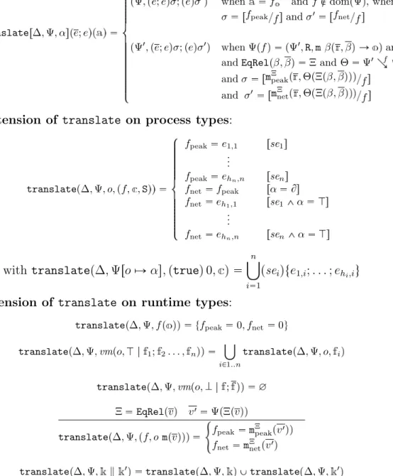
The translation function, called translate, is structured in three parts that respectively correspond to simple atoms, behavioral types, and method types and full programs. This function carries five arguments:

1. is the equivalence relation on formal parameters identifying those that are equal. We assume that x returns the unique representative of the equivalence class of x. For simplicity we also let x x for every x that belongs to the local variables. Therefore we can use also as a substitution operation.

Static analysis of concurrent programs based on behavioral type systems

HAL Id: tel-01660749

https://hal.inria.fr/tel-01660749

behavioral type systems

Abel Celestrín

To cite this version:

DOTTORATO DI RICERCA IN INFORMATICA

Ciclo: XXIX

Static analysis of concurrent programs

based on behavioral type systems

Abstract

Acknowledgements

Contents

I

The static resource analysis problem

9

II

The deadlock analysis problem

69

Chapter 1

Introduction

1.1

Static analysis

1.2

Behavioral type systems based analysis

Generic approach

1.3

Problems tackled in this work

1.4

Aim, objectives, and contribution of this

work

1.4.1

Objectives

1.4.2

Contribution

1.5

Document contents

Part I

The static resource analysis

problem

Chapter 2

Machine usage upper bounds in

vml

Summary

2.1

Introduction

Chapter contents

2.2

Motivation and Problem Statement

Problem statement

2.3

The language vml

2.3.1

Syntax

.

2.3.2

Semantics

.

.

.

2.3.3

Examples

2.4

Determinacy of method’s arguments release

2.5

The behavioral type system of vml

2.6

The analysis of vml behavioral types

2.6.1

Arguments’ identities

2.6.2

(Re)computing argument’s states

2.6.3

The translation function