Preventing iron( II ) precipitation in aqueous systems using polyacrylic acid some molecular insights

HAL Id: cea-02418710

https://hal-cea.archives-ouvertes.fr/cea-02418710

HAL is a multi-disciplinary open access archive for the deposit and dissemination of sci-entific research documents, whether they are

pub-L’archive ouverte pluridisciplinaire HAL, est destinée au dépôt et à la diffusion de documents scientifiques de niveau recherche, publiés ou non,

Preventing iron( II ) precipitation in aqueous systems

using polyacrylic acid some molecular insights

Pierre-Arnaud Artola, Bernard Rousseau, Carine Clavaguera, Marion Roy,

Dominique You, Gabriel Plancque

To cite this version:

Pierre-Arnaud Artola, Bernard Rousseau, Carine Clavaguera, Marion Roy, Dominique You, et al.. Preventing iron( II ) precipitation in aqueous systems using polyacrylic acid some molecular in-sights. Physical Chemistry Chemical Physics, Royal Society of Chemistry, 2018, 20, pp.18056-18065. �10.1039/c7cp02743e�. �cea-02418710�

Preventing iron (II) precipitation in aqueous

systems using Polyacrylic acid: some

molecular insights

Pierre-Arnaud Artola

, Bernard Rousseau

,

Carine Clavagu´era

_,

Marion Roy

_{, Dominique You}

_{, Gabriel Plancque}

February 1, 2017

Abstract

We present Molecular Dynamics simulations of aqueous iron (II) systems in the presence of polyacrylic acid (PAA) under extreme con-ditions that take place in the secondary coolant circuit of nuclear power plant. The aim of this work is to understand how the oligomer can prevent iron (II) deposit and to provide molecular interpretation. We show how, to this purpose, not only the complexant ability is nec-essary but also the chain length compared to iron (II) concentration. When the chain is long enough, a hyper-complexation phenomenon occurs that can explain the specific capacity of the polymer to pre-vent iron (II) to precipitate.

Keywords: Molecular Dynamics, water, iron, polyacrylic acid, sec-ondary circuit, complex, dispersant, Pressurized Water Reactor.

1

Introduction

Energy production is a major issue of the 21st _{century. Many countries have}

opted for nuclear electricity and its safety use feeds public debates. Over the last decade or so, incidents due to the fouling of the Steam Generators (SGs) and the blockage of the tubes support plates have been observed in nuclear power plants. One of the main goals in nuclear industry nowadays is to keep a high level of performance and simultaneously decrease fouling and, therefore, maintenance.

Figure 1: Chemical structure of polyacrylic acid (left) and polyacrylic acetate (right) under basic conditions found in the secondary coolant circuit.

magnetite, in the secondary coolant circuit that can cause deposits very diffi-cult to evacuate, responsible for yield decreases but also for steam generator tubes failures due to excessive vibration fatigue cracking. One of the meth-ods chosen to overcome this problem is to add polyacrylic acid (illustrated on figure 1) in small amount (a few ppb, i.e. a few µg per kg) in the feed water. With this polymer the iron amount extracted by the steam generator blowdown is increased by at least a factor of 5, depending on the amount of polyacrylic acid (later referred as PAA) introduced.

Although very efficient, there is no molecular understanding of this effi-ciency: experiments in extreme conditions (super-critical water state under pressure, typical values are T = 540 K and p = 100 · 105 _{Pa) are very}

diffi-cult to study on the fly and, usually we only have access to the amount of iron (II) extracted but not to chemical and physical phenomenan involved. Two major possibilities are usually presented [1]:

• A complexation effect: carboxylate chemical functions can represent plausible ligands for the iron. This effect has been recently illustrated experimentally [2].

• A dispersant effect: the polymer would play the role of some gigantic surfactant that solvates iron oxide particles.

This issue is obviously very challenging and many related problems can be linked to each possibility. Let us focus for this paper on the first possibility,

∗_{pierre-arnaud.artola@u-psud.fr, Laboratoire de Chimie-Physique, Universit´e de}

Paris-Sud, Orsay, France

†_{Laboratoire de Chimie-Physique, UMR 8000 CNRS, Universit´e de Paris-Sud, Orsay,}

France

the complexation one. It is well known to all chemists that, at ambient conditions, hydroxides and oxides can precipitate with iron (II) more easily than acetates, but there are two important things that need to be taken into account:

• a polymer with many carboxylate functions presents several association sites within the same molecule;

• water thermodynamical conditions in the steam generator go from am-bient to quite extreme (up to 560 K and 7 MPa, at the limit of the vapor liquid equilibrium). In such conditions, the dielectric constant is decreased and ions solvation hability is therefore also decreased;

• we limit our study of iron (II) as hydrazine is currently added in the secondary circuit to be in reducing conditions.

Furthermore, the autoprotolytic constant of water changes a lot within this range of temperature (from 13.995 at 298.15 K to 11.313 at 560.15 K). As a consequence, it is not simple to interpret physico-chemistry in such condi-tions with the polymer as with acetate ions at ambient condicondi-tions.

Lastly, due to extreme experimental conditions, it is very hard to obtain molecular informations from spectroscopic experiments only. This is one of the reason we propose a molecular simulation approach. Similar approaches have already been used, see for instance [3, 4] in which complexes of calcium (II) and polyacrylic acid oligomers have been studied by molecular simula-tions using classical force fields.

In this paper, we present classical molecular dynamics simulations of an oligomer of the acrylic acid in the presence of iron (II) ions. We will first of all present the methods we used, then validate our model and finally present the results of this study.

2

Methodology

This section provides the details of the molecular dynamics used and the quantities obtained from these simulations that are presented in this paper.

2.1

Molecular Dynamics simulations

Molecular dynamics simulations were performed using our locally build New-ton package [5]. The experimental concentrations are too small to be re-produced in simulations with atomistic potentials. Therefore our systems represent oligomer molar concentrations in the range of 1 · 10−2 _{to 5 · 10}−2

mol/kg. Each system contains between 2000 and 5000 water molecules in order to avoid self interaction between PAA molecules. Water molecules are described as rigid species. On the contrary, PAA molecules’ internal degrees of freedom are taken into account, with exception of covalent bond vibra-tions. Bond lengths are contrained using the RATTLE [6] algorithm with a relative tolerance set to 10−10_{. Equations of motion are integrated with the}

explicit reversible velocity Verlet algorithm [7, 8, 9] using a time step chosen as 1 fs. We used a Nos´e-Hoover chain of 10 segments with a time constant value equal to 0.1 ps for NV T simulations. In order to computed equilibrium densities of several systems (see tables 1, 2 and 3), we also performed NpT simulations using the Berendsen thermostat and barostat. The barostat and thermostat time constants were set equal to 0.1 ps.

We performed NV T Nos´e-Hoover [10, 11, 9] molecular dynamics simulations with two propanoates and one iron (II) in 3000 water molecules under ambi-ent and extreme conditions with the densities obtained from our pure water densities. This makes sense for these simulations only as long as the system is at infinite dilution. Then we considered an oligomer of ten monomeric groups and performed MD simulations of this oligomer with 5000 water molecules and respectively 1, 2, 3, 4 and 5 iron (II) ions. In order to ensure electric neutrality, the necessary amount of sodium counter ions was included. Simulations were done in a cubic box using so-called periodic boundary con-ditions and minimum image convention. In order to compute structural prop-erties and mean-squared displacement, trajectory files including particle po-sitions were written every 50 fs.

We used a Lennard-Jones cutoff of 15 ˚A, and an electrostatic cutoff taken as half the box size. Long range interactions for the Lennard-Jones potential were calculated using an homogeneous approximation and long range elec-trostatic interactions were calculated using Ewald summation method [6].

2.2

Monte Carlo simulations

Monte Carlo (MC) simulations were performed using the Gibbs package [12]. All MC simulations were performed with the same initial configurations than the MD simulations. Simulations were performed in both isothermal-isobaric

NpT ensemble and canonical NV T ensemble. The Ewald summation [6]

technique was employed to treat long range electrostatic interactions. The same cutoff were used than in the MD simulations. Simulations were con-ducted as follow: after an equilibration run of 106 _{steps, a production run of}

100 · 106 _steps.

For each MC step, typical moves and associated probabilities are transla-tions (20-25%), rotatransla-tions (20-25%), volume changes (0.5%), stretching (20%),

bending (10%), internal rotations (10%), pivots (5%), twists (5%).

2.3

DFT simulations

2.4

Potential parameters

Water force field: We used the TIP4P 2005 [13] for water. This potential is very common and quite accurate to predict many water properties for pure water and associated mixtures, see for instance (but not restricted to) [14, 15, 16]. We also validated the choice of this force field by several simulations using the SPC/E [17] force field.

polyacrylic acid (n = 1 and n = 10): We used the GROMOS [18] force field for the atactic and fully ionized PAA as this potential proved efficient to model this polymer in the literature [19, 20].

iron (II) : We used the PCFF [21] force field to describe the iron (II) cations.

Na(I): We used the GROMOS [18] force field for the sodium cation. This counter ion is added, if necessary, to ensure electroneutrality.

Cross interactions: Interactions between unlike Lennard-Jones centres were estimated using the so-called Lorentz-Berthelot mixing rules:

σij =

σii+ σjj

2

εij = √εiiεjj

with σ the zero in the Lennard-Jones potential and ε the depth of the potential. Superscripts i and j refer to centre of forces.

Some simulations were performed using geometric mixing rules for both σ and ε in order to study the effect of the mixing rules on the structure of the complexes.

2.5

Radial distribution functions and coordination

num-bers

Radial distribution function (i.e. density probability of finding a particle j at a distance r of an particle i) is noted gij(r) and was calculated as follows:

gij(r) = 1 4πr2_ρ i dN_ij(r) dr ,

with dN_ij(r) the number of species j inside the sphere layer between r and

r + dr around species i and ρi the number density of species i. Although very

informative, these curves are quite difficult to interpret as they are so many of them and it is necessary to interpret several of them (at the same time) to be sure of the molecular interpretation. We consider a simpler (but less) detailed way to analyze the structure: we computed coordination numbers by counting the number of molecules complexing the iron (II) in the first sphere as follows: N_ij = ρi Z _r0 0 4πr2_g ij(r)dr ,

with N_ij the number of particle type i around an particle type j, r0 the

radius of the coordination sphere, gij(r) the radial distribution function

be-tween centres i and j. The r0 value is chosen at the end of the complexation

peak in the radial distribution function.

3

Results and discussion

3.1

Simulated systems

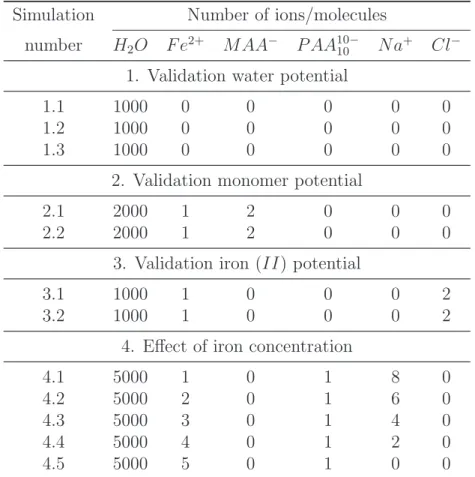
We present on tables 1, 2 and 3, numbers of molecules of each chemical species, thermodynamic conditions, and simulation details. Four different sub-studies were conducted to validate water, polymer, metal force fields and finally to study the effect of iron (II) concentration.

3.2

Potential validation

3.2.1 Water force field

The system we are interested in is mainly constituted by water molecules. Therefore a good thermodynamical description of pure water in high tem-perature and high pressure conditions is required. We performed MD and MC simulations at ambient conditions (298.15 K and 105 _{Pa) and also at}

ex-treme conditions (543.15 K and 100·105 _{Pa). In the latter we chose a pressure}

slightly greater than the vapor liquid equilibrium one to avoid phase separa-tion in the simulasepara-tion box. Large systems are simulated (simulasepara-tions 1.1, 1.2

Simulation Number of ions/molecules

number H2O F e2+ MAA− P AA10−10 Na+ Cl−

1. Validation water potential

1.1 1000 0 0 0 0 0

1.2 1000 0 0 0 0 0

1.3 1000 0 0 0 0 0

2. Validation monomer potential

2.1 2000 1 2 0 0 0

2.2 2000 1 2 0 0 0

3. Validation iron (II) potential

3.1 1000 1 0 0 0 2

3.2 1000 1 0 0 0 2

4. Effect of iron concentration

4.1 5000 1 0 1 8 0

4.2 5000 2 0 1 6 0

4.3 5000 3 0 1 4 0

4.4 5000 4 0 1 2 0

4.5 5000 5 0 1 0 0

Table 1: Summary of the number of each chemical species of all simulated systems. Acronyms MAA− _{and P AA}10−

10 refer respectively to proprionate

and polyacrylic carboxylate ions

and 1.3) to ensure the validity of the results. MD NpT simulations are per-formed as follow: after a quick volume rescalling in order to put the system close to experimental densities, 1 nanosecond of equilibration followed by 20 nanoseconds of production on 2000 water molecules. MC NpT simulations are performed as follow: from the same initial box than MD simulations, a first equilibration run of 106 _{steps is done, followed with a production run of}

100 · 106 _steps.

We present on figure 2 the densities of the simulated pure water systems under 100 · 105 _{Pa at three temperatures. Several papers already present}

efficiency of the TIP4P 2005 water potential under various and in particular high temperature and pressure conditions, see for instance [22]. Neverthe-less, we tested TIP4P 2005 force field and compared to SPC/E [17] force field which is optimized to be used with the GROMOS force field, the force

Simulation Thermodynamic state number T (K) p (MPa) ρ (kg/m3₎

1. Validation water potential

1.1 473 10.0 ± 0.06 863.94 ± 0.07 1.2 498 10.0 ± 0.07 832.09 ± 0.11 1.3 523 10.0 ± 0.06 796.60 ± 0.09

2. Validation monomer potential

2.1 298 0.099 ± 0.04 1001.1 ± 0.1 2.2 543 10.0 ± 0.04 765.5 ± 0.1

3. Validation iron (II) potential

3.1 298 0.054 ± 0.11 1011.3 ± 0.1 3.2 543 10.0 ± 0.04 776.1 ± 0.1

4. Effect of iron concentration 4.1 543 7.22 ± 0.09 766.8 4.2 543 7.20 ± 0.17 766.8 4.3 543 6.93 ± 0.18 766.8 4.4 543 7.32 ± 0.12 766.8 4.5 543 7.33 ± 0.08 766.8

Table 2: Thermodynamic conditions of all simulated systems

field chosen for the PAA oligomer. The densities are confronted to experi-mental data correlation [23]. Simulated densities are always smaller than the experimental correlation values, which is expected for thermodynamical con-ditions quite close to the critical temperature. The densities obtained with the TIP4P 2005 force field are in good agreement, with an error below 0.8%. On the contrary, the values obtained with the SPC/E force field are always below the target values with an error of, at least, 3.8%. Given these results, one may expect the TIP4P 2005 potential to describe in a better way the structure and thermodynamical properties of water under such conditions.

3.2.2 Iron (II) force field

Before going into the full system (water molecules, iron (II) ions and PAA oligomers), we consider the system of the water molecules and the iron (II) ions and chloride counter-ions (simulations 3.1 and 3.2). Various

experimen-Simulation Simulation details

number Statistical ensemble Equilibration time Production time 1. Validation water potential

1.1 NpT 2 ns 15 ns

1.2 NpT 2 ns 15 ns

1.3 NpT 2 ns 15 ns

2. Validation monomer potential

2.1 NpT 1 ns 15 ns

2.2 NpT 1 ns 15 ns

3. Validation iron (II) potential

3.1 NpT 1 ns 6 ns

3.2 NpT 1 ns 6 ns

4. Effect of iron concentration

4.1 NV T 1 ns 5 ns

4.2 NV T 1 ns 5 ns

4.3 NV T 1 ns 5 ns

4.4 NV T 1 ns 5 ns

4.5 NV T 1 ns 5 ns

Table 3: Summary of simulation types of all simulated systems

tal data (see for instance [24]) present typical distances between water oxygen atoms and iron (II) ions. These values are compared to the simulated values in table 4. Simulations were performed with water molecules described by the TIP4P 2005 force field. First of all we observe that iron (II) cation is

T (Kelvin) dOw−Fe NOFew

298 (this work) 1.95˚A 6.00 543 (this work) 1.90˚A 4.23 298 (exp) 2.00˚A 6.00

Table 4: Oxygen-iron (II) distances and coordination numbers (average num-ber of water oxygens around an iron (II) ion) obtained from our simulations and compared to experimental data [24].

470

480

490

500

510

520

530

T (K)

760

780

800

820

840

860

880

900

ρ

(kg/m

)

IAPWS

TIP4P/2005

SPCE

Figure 2: Density-temperature simulated curve of the TIP4P 2005 and SPC/E water models compared to experimental data correlation [23] un-der a pressure of p = 10 MPa. Statistical errors are of the orun-der or smaller than symbol size.

hexa-coordinated in our simulations, as it is in experiments [24] under ambi-ent conditions. Under extreme conditions (543 K and pressures from table 2), there are only, approximately, 4 water molecules but also two chloride ions. This neutral structure is more stable as, under high temperature conditions, dielectric constant of water is decreased significantly (εr ≈ 24.2 obtained

from IAWPS correlation [23]). The obtained values with a simple force field in which electrostatic interactions are described by single point charges are in good agreement with experimental distances.

3.2.3 Full system description

General observations: In order to validate the structure with the oligomer, we consider the same kind of simulations in which we replace the two chlo-rides by two propanoates. The related simulations are described as simu-lations 3.1 and 3.2 in tables 1, 2 and 3. We compare the structure under extreme conditions with the one obtained from reference [25]. The systems are not equivalent, but the molecules studied in [25] also contains a carboxy-late group which complexes the iron (II) . As can be observed on table 5, there is quite a good agreement in the structures even though they cannot be compared directly as the systems are different and under different thermody-namic conditions. Nevertheless, typical structures of complexes, than could be observed on snapshots and compared to the one given in reference [25] are very similar. Furthermore the structure of the complex, in which the

T (Kelvin) dOw−Fe N

Fe

Ow dOate−Fe NOFe_ate

543 (this work) 1.96˚A 2.30 1.96˚A 4.00 298 (ref [25]) 2.00˚A 1.99 2.00˚A 4.00

Table 5: Oxygen-iron (II) distances and coordination numbers (average num-ber of water and carboxylate oxygens around an iron (II) ion) obtained from our simulations and compared to other MD data [25].

carboxylate groups do not form a square with the iron (II) cation in the midle, but an asymetric structure is similar to what has been observed with equivalent systems with MD [25]. We will go into more quantitative analysis in the next paragraphs.

Comparaison with DFT simulations: In order to validate the choice of simple models to describe complex interactions, we compared, for one sys-tem, the MD simulations of the oligomer with 5 iron (II) ions with quantic simulations.

The geometry of the system, one oligomer plus 5 Fe(II) ions (95 atoms), was optimized at the DFT level with the PBE0-D3 functional and the def2-SVP basis set. There is no major change in the gas phase geometry in compari-son with the structure surrounded by water, except rearrangement of the O atoms around Fe atoms.

The geometry was re-optimized using a COSMO model [26, 27] and a dielec-tric constant of 24.1898 obtained from the IAWPS correlation. The geometry changes are very minor and are illustrated on figure 3.

Figure 3: Structure optimized of the oligomer and 5 ions from DFT simula-tions

The bonding energy of the system has been decomposed into various con-tributions based on two fragments: one for Fe2+ _{(54) and one for the oligomer}

+ 4 Fe2+ _{(PBE0-D3/TZP level). All energetic terms are given in table 6.}

(kcal/mol) Egas Esolv

Pauli repulsion 494.2 492.6 Electrostatic -609.3 -607.7 Orbital interactions -852.3 -841.1 Dispersion -5.8 -5.8 Solvation -61.3 Total bonding energy -973.2 -1023.3

Table 6: Energy decomposition of the oligomer plus 5 ions obtained from the DFT simulations.

Please note that energetic values in table 6 cannot be compared directly to values reported in reference [3] as methods used to compute energies of the complex are completely different.

Effect of mixing rules on the structure of the system: We chose the GROMOS force field for the polyacrylic acid oligomers, and this force field has been optimized with SPC/E force field and geometric mixing rules.

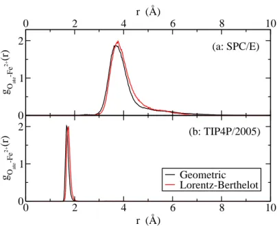
In order to test these last aspects, we performed MC and MD simulations 2.1 and 2.2 with TIP4P 2005 and SPC/E water models (see table 1), and for both force fields, we tested both geometric and Lorentz-Berthelot mix-ing rules. We present on figure 4 the radial distribution functions between the oxygens of the carboxylates and the iron (II) ions for simulation 2.2. First of all we observe almost no effect at all of the mixing rule on the dis-tributions. Furthermore, the coordination distance observed with SPC/E water molecules is approximately equal to 3.8 ˚A, which is not a typical co-ordination value for a complex, and with a large distribution in distances. We can interpret this feature as the iron (II) ion is complexed only by the water molecules, even though the electrostatic interactions should favored the complexation by the propanoate molecules. We analyse this difference as follows: the SPC/E water potential has a negative charge on the oxygen whereas in the TIP4P 2005 water potential the negative charge is shifted towards hydrogens. As the complex formation in our simulations arises from electrostatic interactions, when the negative charge of water models are at the same distance from iron (II) , repulsion is much more important with the TIP4P 2005 model. We observe that the propanoate molecules cannot complex the iron (II) ions in the SPC/E water molecules “bath”. Therefore, we performed all the production simulations with the TIP4P 2005 model.

Thus, the models we consider here seem to give reliable results considering the structure of the fluid under extreme conditions and the iron (II) complex, which is precisely what we are interested in.

3.3

Effect of the iron (II) concentration

Before going into the details of the results, we mention that simulated concen-trations are considerably larger than experimental conditions. Nevertheless, as we are interested in statistical equilibrium and thermodynamical proper-ties, one may expect a good extrapolation to more dilute systems.

As we already mentioned, when added, the polymer PAA has a great im-pact on the iron (II) removal, and on the contrary, the acetate has not [1]. This obviously suggests that there is a specificity of the polymer. In or-der to unor-derstand how the chain of the polymer affects the structure, and consequently the ability to complex the iron cation, we present on figure 5 the radial distribution functions between the iron cation and the carboxylate oxygens for the various tested concentrations of iron cations. We clearly see a first very intense peak for small distances, in a range of 1.7 − 1.8 ˚A. For greater distances (up to 2.8 − 3.0 ˚A) the radial distribution function almost vanishes. This peak represents then the complex between the iron (II) and the carboxylate oxygens. This indicates that the polymer has the ability

0 2 4 6 8 10 r (Å) 0 1 2 g O ate -Fe 2+ (r) 0 2 4 6 8 10 r (Å) 0 1 2 g O ate -Fe 2+ (r) Geometric Lorentz-Berthelot (a: SPC/E) (b: TIP4P/2005)

Figure 4: Simulated system 2.2 (see table 1): comparison between (a) SPC/E and (b) TIP4P 2005 force fields with geometric and Lorentz-Berthelot cross interaction mixing rules

to complex the iron (II) cations. For larger intermolecular distances (from 3.0 ˚A to “∞”) we observe a distribution of peaks. Two important remarks emerge: the intensity of the distribution is very small compared to the com-plexing peak and the shape changes with the iron concentration as it must affects the oligomer conformation. This indicates there is almost no exchange between oligomer and water molecules in this concentration regime. Different behaviour may be expected for large iron (II) contentrations.

An interesting feature that can be seen on figure 5 is that there is not a monotonic evolution of intensities of the first peak of radial distribution functions. We will come back to this point later in the paper.

Another interesting issue is to compare the carboxylate oxygens to water oxy-gens. We present on figure 6 radial distribution functions between iron (II) cations and water oxygens.

We observe the same kind of behaviour: some water molecules are in-cluded in the cluster but in a different manner than the carboxylate functions of the polymer. Indeed, the typical distances are here 1.9 − 2.0 ˚A and with a much larger distance distribution for the cluster. This indicates a greater lability of the complexing water molecules compared to the carboxylate

func-1.6 2 2.4 2.8 r (Å) 0 2 4 6 8 g O ate -Fe 2+ (r) n Fe2+ = 1 n Fe2+ = 2 n Fe2+ = 3 n Fe2+ = 4 n_Fe2+ = 5 0 5 10 15 0 0.1 0.2

Figure 5: Radial distribution functions between iron (II) cations and car-boxylate oxygens for a number of iron (II) ions going from 1 to 5. The main figure presents a distance range focused on the first coordination sphere of the iron (II) complex and the encapsulated figure the structure over the entire distance range.

tions.

Although the peak height may vary a lot, let us note here that it is the inte-grated radial distribution function that is correlated to a coordinance number and not only the height of the first peak.

3.4

Oligomer conformation

As we mentioned above, the conformation of the oligomer is affected by the complexation and iron concentration. An interesting feature is to predict whether two adjacent carboxylate groups complex the iron. For this pur-pose, we consider saturated oligomer (simulation 4.5). In the data analysis, we differentiate carboxylate oxygens whether they belong to an even or an odd monomeric group, meaning its position along the chain. Two possible structures can be imagined:

1.6 2 2.4 2.8 r (Å) 0 4 8 12 g O w -Fe 2+ (r) 0 2 4 6 8 10 0 4 8 12 n_Fe2+ = 1 n_Fe2+ = 2 n Fe2+ = 3 n Fe2+ = 4 n Fe2+ = 5

Figure 6: Radial distribution functions between iron (II) cations and water oxygens for a number of iron (II) ions from 1 to 5. The main figure presents a distance range focused on the first coordination sphere of the iron (II) complex and the encapsulated figure the structure over the entire distance range.

• Each iron (II) is complexed from two successive even or odd oxygens, in which case, the distances between two successive even or odd carboxy-late groups would be smaller than the distance between two successive carboxylate groups.

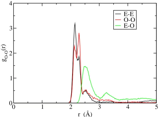
We present on figure 7 the three radial distribution functions between two oxygens (odd-odd, even-even, and odd-even). The even-even (E − E) radial distribution function is very similar to the odd-odd (O − O) one, which is what was expected. We clearly observe that the first peak of the E − E and the O − O distributions appears at a smaller distance than the first peak of the O − E radial distribution function. The most plausible reason is that iron (II) is complexed by two adjacent odds or evens carboxylate groups.

Although thermodynamical conditions are very different, this observation is very similar to what have been observed by Bulo et. al. [3] with complexes of PAA oligomers and calcium (II) cations: a structure in which the chain complexes cations with two adjacent carboxylate functions is less stable than when the carboxylate functions are not adjacent. Following the authors, and

0

1

2

3

4

5

r (Å)

0

1

2

3

4

g

(r)

E-E

O-O

E-O

Figure 7: Radial distribution functions between two oxygens of the oligomer whether they belong to an even or an odd carboxylate group. Subscripts “O” and “E” refer respectively to “odd” and “even” positions in the chain.

what have been already reported by Sinn et. al. [28] for the calcium (II) cation and, for instance, by Burrows et. al. [29] for aluminium (III) and chromium (III) cations, complexation by oligomers, and consequently by longer polymers, has a strong entropic contribution even under such thermo-dynamical conditions.

3.5

Quantitative analysis

In order to have a more quantitative description of the local structure of the system, we computed coordination numbers. Before going into the result details, we need to precise to what we correlated the coordination numbers. What is important is not only the molar quantity of carboxylate chemical

functions added in the system at a given molar concentration of iron (II) but rather the length of the polymer at a given molar concentration of iron (II) . This defines some control parameter ψn−F e as:

ψn−F e = n

[PAAn]

[F e2+_] ,

with n the polymerization degree, which can be estimated simply from the total molar mass of the polymer and the molar mass of a single monomer, [F e2+_{] the iron (II) molar concentration and [PAA}

n] the molar concentration

of PAA. This parameter is an indication of the length of the polymer at a given experimental iron (II) concentration. In the following, we refer to this parameter as the relative complexant ability parameter (RCAP).

In our simulations, as we consider finite size systems and a single oligomer chain, it is easier to define a simplified parameter as:

φn−F e = n

Nb (F e2+₎,

with Nb(F e2+_{) the number of iron (II) included in the simulation. This}

simulated parameter is referred as the reduced relative complexant ability parameter (rRCAP).

We present on figure 8 the coordination numbers of all oxygen types and the total as functions of the reduced relative complexant ability parameter. The first interesting result of this figure is the total coordination number of oxygen around an iron (II) cation: it is pretty much constant and its average is:

D

NbF e_Oall2+

E

φ = 5.57 ,

where < . >φ represents the average over all φ values. This value is

slightly smaller than what we observed with the monomer (5.95) obtained from our simulations. The explanation comes from the value of the coordi-nation number of carboxylate oxygen at large reduced relative complexant ability parameter: it is almost equal to 5. This indicates a specific ability of the polymer to form a hyper-complex tridentate (and each carboxylate ligand has two oxygens). As a consequence, at large reduced relative complexant ability parameter values, even if the iron (II) has already two carboxylate functions in the complex, the two last positions in the complex are rather occupied by another carboxylate function than a water molecule.

Let us stress here that this behaviour is only possible if there is at least three carboxylate groups for each iron (II) cation.

2

4

6

8

10

12

φ

0

1

2

3

4

5

6

Nb

O

O

O

φ

= 3.34

Figure 8: Coordination numbers of all oxygen types around iron (II) cation obtained under extreme conditions (543K). The oxygen subscripts “ate”, “w” and “all” refer to the oxygens in PAA molecules, water molecules, and both of them, respectively.

that there is some inversion between the two coordination oxygens, and the water oxygens seem to complex in a better manner the iron (II). Here we encounter a finite size effect as there are three iron (II) cations in the simulations. We observed that the polymer “tries” to hyper-complex one of them, which leaves four carboxylate groups for the two remaning iron (II) cations. Furthermore two adjacent carboxylate groups cannot complex the same iron (II) cation. As a consequence, in this specific system, there is one hyper-complexed iron (II) cation, and the two others are complexed by one carboxylate group and water fills the holes. So the inversion is due to finite size oligomer but we can explain it from the general behaviour. In order to illustrate this specific structure, we present on figure 9 a structure

of the system with three iron (II) cations and compare with the structure with a single iron (II) cation. We clearly identify in the two examples the hyper complexed structure. Due to this and also to the small chain length of our oligomer, the two other iron (II) cations have only a single carboxylate group left for each of them.

Figure 9: Left: Typical structure of the simulated system with three iron (II) cations. Right: Typical structure of the simulated system with one iron (II) cation. Figures only present the oligomer and iron (II) cations. Iron (II) ions are presented in black.

As a consequence of these simulations, we may propose a molecular inter-pretation of the action of the polymer in realistic situations: under extreme thermodynamic conditions the water dielectric constant is significantly de-creased, therefore solvation of ions is less favourable. As had already reported in the literature (see for instance [20]), the structure of the polymer is strongly affected by the solution charges. As a consequence, in our case, as temper-ature changes dramatically the permitivity constant of water, the polymer chains under ambient conditions are essentially depleted and consequently less able to complex iron (II) cations, but under higher temperatures, the polymer chains structure fold up and it increases the complexant ability. The specificity of the polymer is that it can, within a single molecule, offer all the complexant groups needed in a small region of space under high temperature. Furthermore, if the reduced relative complexant ability parameter is above 3.5 approximately, the system is in such conditions that the polymer can hy-per complex the iron (II) cations. This might be the clue to the effect of the polymer in the nominal operating conditions of the secondary circuit. This

provides a molecular interpretation of the complexation mecanism observed experimentally [2]. This hyper-complexant hability of the polymer under high temperature seems to be specific to these thermodynamical conditions, as a four-coordinated stable structure has been reported under ambient con-ditions [3].

Following what has been described in reference [4], in which a comparison between a situation with a single polymer and two polymers has been inves-tigated, equilibrium structures can be significantly different. Nevertheless, when a second chain is added, the total complexant ability, i.e. the total number of carboxylate functions, is doubled, and one should compare the 10 mer with two 5 mers. We are currently invistigated this effect with simula-tions of a 20 mer compared to two 10 mers and 20 monomers.

3.6

Minimal efficient chain length

In the steam generator, most (99 %) of the liquid of the secondary coolant circuit is vaporized, therefore, iron (II) concentration is increased a hundred times up to:

£

F e2+¤_{= 10}−8_mol/kg,

Experiments have already shown that the PAA chain length decreases due to thermal degradation as the residence time in the steam generator increases[30]. We showed that the φn−F e (and so ψn−F e) parameter should

be greater than, at least, 3.33. We choose here a value of 20 to be clearly in the hyper complexation regime. Furthermore, the polymer is included in a very small amount in the steam generator. We consider the limit of efficiency of the polymer, when degraded several times, so plausible values of concentrations could be:

[polymer] [F e2+_] ≈ 0.1

The corresponding minimal efficient chain length is then given by:

ψn−F e = nmin

[polymer] [F e2+_]

so

nmin ≈ 200

Obviously, the product nmin[polymer] is almost constant as when the

concentration of the polymer increases when degraded, its length is divided by the same factor. As a consequence, it is required to have, to start, the greater

possible chain length of the polymer, and knowing the limiting efficiency value with the molecular mass distribution of the degraded polymer [31], this could be a way to predict the efficient time of the polymer in the steam generator.

4

Conclusions and further work

In this paper, we presented Molecular Dynamic simulations of the effect of a PAA oligomer injected in the secondary coolant circuit of nuclear power plant to prevent iron precipitation and deposition in steam generators. We proposed a molecular interpretation of the complexation mechanism of the polymer in the presence of the iron (II) under extreme thermodynamic con-ditions. We identify the length of the polymer as a clue parameter to combine to the complexant ability of carboxylate groups all along the chain.

The polymer is able to “hyper” complex iron (II) cations by encapsulating them, but on the condition there are enough carboxylate functions for each iron (II) . In order to quantify this more precisely, we propose a parameter RCAP that links the chain length (meaning the carboxylate group number) to the relative number of iron (II) inside the system.

Further investigation of the hyper complexation changing the rRCAP pa-rameter would be required in order to investigate a “phase diagram” figure defining precisely the minimal chain length for efficiency.

Finally, we should also investigate the balance between the complexation equilibrium with the precipitation with hydroxide ions for various concentra-tions of ions and various chain lengths of the polymer.

References

[1] Mercier, St´ephane and Corredera, G´eraldine and Alves-Vieira, Maria and Mansour, Carine and You, Dominique. EDF Plan For a Dispersant Injection Trial. In Nuclear Plant Chemistry Conference, 2012.

[2] Roy, M. and Mansour, C. and You, D. The Effect of Polyacrylic Acid on Iron Oxides Formed on Steam Generator Tubes and on Metallic Copper Present in Pressurized Water Reactors. In Nuclear Plant Chemistry

Conference, 2014.

[3] Rosa E. Bulo, Davide Donadio, Alessandro Laio, Ferenc Molnar, Jens Rieger, and Michele Parrinello. ”site binding” of ca2+ ions to polyacry-lates in water: A molecular dynamics study of coiling and aggregation.

[4] Gareth A. Tribello, CheeChin Liew, and Michele Parrinello. Binding of calcium and carbonate to polyacrylates. The Journal of Physical

Chemistry B, 113(20):7081–7085, 2009.

[5] V.-O. Nguyen-Thi, C. Houriez, and B. Rousseau. Viscosity of the 1-ethyl-3-methylimidazolium bis(trifluoromethylsulfonyl)imide ionic liq-uid from equilibrium and nonequilibrium molecular dynamics. Physical

Chemistry Chemical Physics, 12(4):930–6, January 2010.

[6] M. P. Allen and D. J. Tildesley. Computer simulation of liquids. Oxford Science publications, Oxford, 1989.

[7] Loup Verlet. Computer ”experiments” on classical fluids. i. thermody-namical properties of lennard-jones molecules. Phys. Rev., 159:98–103, 1967.

[8] D. Levesque and L. Verlet. Molecular dynamics and time reversibility.

Journal of Statistical Physics, 72(3-4):519–537, 1993.

[9] G. J. Martyna, M. Tuckerman, D. Tobias, and M. Klein. Explicit re-versible integrators for extended systems dynamics. Molecular Physics, 87(5):1117–1157, April 1996.

[10] Nos´e, Shuichi. A unified formulation of the constant temperature molec-ular dynamics methods. The Journal of Chemical Physics, 81(1):511– 519, 1984.

[11] W.G. Hoover. Canonical dynamics: Equilibrium phase-space distribu-tions. Physical Review A, 31(3):1695–1697, 1985.

[12] Ungerer, P. and Tavitian, B. and Boutin, A. Applications of Molecular

Simulation in the Oil and Gas Industry: Monte Carlo Methods. Editions

Technip - IFP Publications, Paris, France, 2005.

[13] J L F Abascal and C Vega. A general purpose model for the con-densed phases of water: TIP4P/2005. The Journal of Chemical Physics, 123(23):234505–234512, 2005.

[14] Helena L. Pi, Juan L. Aragones, Carlos Vega, Eva G. Noya, Jose L.F. Abascal, Miguel A. Gonzalez, and Carl McBride. Anomalies in water as obtained from computer simulations of the tip4p/2005 model: den-sity maxima, and denden-sity, isothermal compressibility and heat capacity minima. Molecular Physics, 107(4-6):365–374, 2009.

[15] Miguel Angel Gonz´alez and Jos´e L. F. Abascal. The shear viscosity of rigid water models. The Journal of Chemical Physics, 132(9):096101, 2010.

[16] P.-A. Artola, A. Raihane, C. Crauste-Thibierge, D. Merlet, M. Emo, C. Alba-Simionesco, and B. Rousseau. Limit of miscibility and nanophase separation in associated mixtures. The journal of physical

chemistry. B, 117(33):9718–27, August 2013.

[17] H. J. C. Berendsen, J. R. Grigera, and T. P. Straatsma. The missing term in effective pair potentials. The Journal of Physical Chemistry, 91(24):6269–6271, 1987.

[18] Chris Oostenbrink, Alessandra Villa, Alan E. Mark, and Wilfred F. Van Gunsteren. A biomolecular force field based on the free enthalpy of hydration and solvation: The gromos force-field parameter sets 53a5 and 53a6. Journal of Computational Chemistry, 25(13):1656–1676, 2004.

[19] Dirk Reith, Beate M¨uller, Florian M¨uller-Plathe, and Simone Wiegand. How does the chain extension of poly (acrylic acid) scale in aqueous solu-tion? a combined study with light scattering and computer simulation.

The Journal of Chemical Physics, 116(20):9100–9106, 2002.

[20] Muralidharan S. Sulatha and Upendra Natarajan. Origin of the differ-ence in structural behavior of poly(acrylic acid) and poly(methacrylic acid) in aqueous solution discerned by explicit-solvent explicit-ion md simulations. Industrial & Engineering Chemistry Research,

50(21):11785–11796, 2011.

[21] Huai Sun, Stephen J. Mumby, Jon R. Maple, and Arnold T. Hagler. An ab initio cff93 all-atom force field for polycarbonates. Journal of the

American Chemical Society, 116(7):2978–2987, 1994.

[22] C. Vega, J. L. F. Abascal, M. M. Conde, and J. L. Aragones. What ice can teach us about water interactions: a critical comparison of the performance of different water models. Faraday Discuss., 141:251–276, 2009.

[23] Wagner, W. and Pruß, A. The IAPWS Formulation 1995 for the Thermodynamic Properties of Ordinary Water Substance for General and Scientific Use. Journal of Physical and Chemical Reference Data, 31(2):387–535, 2002.

[24] Hitoshi. Ohtaki and Tamas. Radnai. Structure and dynamics of hydrated ions. Chemical Reviews, 93(3):1157–1204, 1993.

[25] Ludmilla Aristilde and Garrison Sposito. Molecular modeling of metal complexation by a fluoroquinolone antibiotic. Environmental Toxicology

and Chemistry, 27(11):2304–2310, 2008.

[26] A. Klamt. Conductor-like screening model for real solvents: A new approach to the quantitative calculation of solvation phenomena. The

Journal of Physical Chemistry, 99(7):2224–2235, 1995.

[27] A. Klamt and V. Jonas. Treatment of the outlying charge in continuum solvation models. The Journal of Chemical Physics, 105(22):9972–9981, 1996.

[28] Cornelia G. Sinn, Rumiana Dimova, and Markus Antonietti. Isother-mal titration calorimetry of the polyelectrolyte/water interaction and binding of ca2+: Effects determining the quality of polymeric scale in-hibitors. Macromolecules, 37(9):3444–3450, 2004.

[29] Hugh D. Burrows, Diana Costa, M. Luisa Ramos, M. da Graca Miguel, M. Helena Teixeira, Alberto A. C. C. Pais, Artur J. M. Valente, Mar-garida Bastos, and Guangyue Bai. Does cation dehydration drive the binding of metal ions to polyelectrolytes in water? what we can learn from the behaviour of aluminium(iii) and chromium(iii). Phys. Chem.

Chem. Phys., 14:7950–7953, 2012.

[30] Lamouroux, C. and You, D. and Plancque, G. and Roy, M. and Laire, C. and Schnongs, P. Assessment of the PolyAcrylic Acid for an Ammonia Water Treatment and for Alloy 800NG SG Tube Material in Pressurized Water Reactors. In Nuclear Plant Chemistry Conference, 2012.

[31] L L´epine and R Gilbert. No Title. Polymer Degradation and Stability, 75(2):337–345, 2002.