Foraminiferal responses to major Pleistocene paleoceanographic changes in the southern South China Sea

HAL Id: hal-03118508

https://hal.archives-ouvertes.fr/hal-03118508

Submitted on 22 Jan 2021

HAL is a multi-disciplinary open access

archive for the deposit and dissemination of

sci-entific research documents, whether they are

pub-lished or not. The documents may come from

teaching and research institutions in France or

abroad, or from public or private research centers.

L’archive ouverte pluridisciplinaire HAL, est

destinée au dépôt et à la diffusion de documents

scientifiques de niveau recherche, publiés ou non,

émanant des établissements d’enseignement et de

recherche français ou étrangers, des laboratoires

publics ou privés.

Foraminiferal responses to major Pleistocene

paleoceanographic changes in the southern South China

Sea

Zhimin Jian, Pinxian Wang, Min-Pen Chen, Baohua Li, Quanhong Zhao,

Christian Bühring, Carlo Laj, Hui-Ling Lin, Uwe Pflaumann, Yunhua Bian, et

al.

To cite this version:

Zhimin Jian, Pinxian Wang, Min-Pen Chen, Baohua Li, Quanhong Zhao, et al.. Foraminiferal

re-sponses to major Pleistocene paleoceanographic changes in the southern South China Sea.

Paleo-ceanography, American Geophysical Union, 2000, 15 (2), pp.229-243. �10.1029/1999PA000431�.

�hal-03118508�

PALEOCEANOGRAPHY, VOL. 15, NO. 2, PAGES 229-243, APRIL 2000

Foraminiferal

responses

to major Pleistocene

paleoceanographic

changes

in the southern

South

China Sea

Zhimin

Jian,

•' 2 Pinxian

Wang,

• Min-Pen

Chen,

3 Baohua

Li,

4 Quanhong

Zhao,

•

Christian

Biihring,

s Carlo

Laj,

6 Hui-Ling

Lin,

7 Uwe

Pflaumann,

s Yunhua

Bian,

•

Rujian

Wang

• and

Xinrong

Cheng

•

Abstract.

A detailed

age

model

for

core

17957-2

of the

southern

South

China

Sea

was

developed

based

on

b•80,

coarse

fraction,

magnetostratigraphy,

and

biostratigraphy

for

the

last

1500

kyr.

The

b•80

record

has

clear-100-kyr

cycles

after

the

Mid-Pleistocene

Revolution

(MPR)

at the

entrance

of marine

isotopic

stage

(MIS)

22.

Planktonic

foraminifera

responded

to

the

MPR

immediately,

showing

the

increased

sea

surface

temperature

(SST)

and

dissolution

after

the

MPR.

Benthic

foraminifera

did

not

respond

to it until

the

Brunhes/Matuyama

boundary.

Since

the

MPR,

the

depth

of thermocline

gradually

became

shallower

until

MISs

6-5. This

major

change

within

MISs

6-5 was

also

reflected

in the decreased

SSTs

and

increased

productivity

and

Deep

Water

Mass.

Thus

two

major

Pleistocene

paleoceanographic

changes

were

found:

One

was

around

the

MPR;

the

other

occurred

within

MISs

6-5,

which

speculatively

might

be

ascribed

to the

reorganization

of surface

and

deep

circulation,

possibly

induced

by tectonic

forces.

1. Introduction

As a marginal sea the South China Sea (SCS) has sedimentation rates higher by an order of magnitude than the Pacific, and its widespread carbonate sediments provide an ideal basis for

high-resolution

paleoceanographic

reconstruction

[Wang

et al.,

1995]. The first cores in the world ocean used for high-resolution stratigraphy documented by accelerator mass spectrometer (AMS) •4C datings were from the southern part of this basin [Andtee et al., 1986; Broecker et al., 1988]. Since the 1980s, marine geologists in

China and abroad have shown growing interest in late Quaternary

paleoceanographic

history

of the

SCS,

for example,

the

changes

in

sea surface temperature (SST) [Wang and Wang, 1990; Miao et al., 1994; Pfiaumann and dian, 1999], productivity [Winn et al., 1992;

Thunell et al., 1992; dian et al., 1999], deepwater conditions

[Berger, 1987; dian and Wang, 1997], carbonate cycles [Wang et al., 1986; Thunell et al., 1992; Wang et al., 1995], monsoon variations [Sun and Li, 1999; Wang et al., 1999], and

paleoenvironmental

interactions

between

land

and

sea

[Wang

and

2Now at Institut flir Geowissenschaften, Universit•it Kiel, Kiel,

Germany

3Institute of Oceanography, Taiwan University, Taipei, China. 4Nanjing Institute of Geology and Paleontology, Academia Sinica,

Nanjing, China.

5Institut far Geowissenschaften, Universit•it Kiel, Kiel, Germany. 6Laboratoire des Sciences du Climat et de 1' Environment, CNRS-CEA,

Gif sur Yvette, France.

7Institute of Marine Geology, Sun Yat-Sen University, Kaohsiung, Taiwan, China.

Copyright 2000 by the American Geophysical Union Paper number 1999PA000431.

0883-8305/00/1999PA000431 $12.0 0

Sun, 1995; Wang, 1999] during the last glacial-interglacial cycle. On the other hand, the high sedimentation rate in the SCS has hindered the Pleistocene paleoceanographic studies because no

core has penetrated

the last two glacial cycles.

The long

come from industrial exploratory wells, engineering geological drill holes and coral reef deposits, which hardly provide continuous and detailed paleoenvironmental records [e.g., Zhang et al., 1996]. Therefore long-term Pleistocene paleoenvironmental records from the China coast are not yet available to be compared

with those recorded in the Chinese loess [Kukla and An, 1989; Liu

and Ding, 1993; Ding et al., 1994], despite

their primary

importance

in our understanding

of the East Asian

paleoenvironmental evolution.

The surface water masses and hydrography in the SCS are

largely

controlled

by the seasonally

reversing

monsoonal

wind

system,

which

causes

drift

currents

to change

their

flow

direction

[Wyrtki,

1961

]. According

to Levitus

and

Boyer

[ 1994],

the

SST

of

the SCS

ranges

from 20

ø to 28.8øC

during

the northeast

winter

monsoon,

with steep

gradients

toward

the coast

of China.

During

29øC. The annual average depth of thermocline (DOT) in the SCS

ranges

from

--.25

m in the

inner

shelf

to --.200

m toward

the

western

Pacific,

primarily

responding

to the wind-driven

cyclonic

surface

circulation

(i.e., Ekman

pumping).

For more

detailed

information

on the modem geographic variations of the SSTs and DOT in the SCS, see Chen et al. [1998] and Pfiaumann and dian [1999]. However, during the glacial period the SCS became a

semienclosed basin connected to the western Pacific through the Bashi Strait and to the Sulu Sea through the Balabac and Mindoro

Straits

due

to the

sea

level

drop

[Wang

et al., 1995].

•his

inevitably

led to a pronounced

difference

in surface

and deep

circulation

[Wang

et al., 1995;

dian

and Wang,

1997]

and

hence

altered

the

upper water structure and deep water conditions.

The northern part of Nansha Islands area ("Dangerous Ground"), the northern slope of the SCS deep basin, is

230 JIAN ET AL.: MAJOR PLEISTOCENE PALEOCEANOGRAPHIC CHANGES distinguished by its very low sedimentation rate because of the

limited access of terrigenous material and may provide continuous and long Pleistocene deep-sea sediment sequences [Sarnthein et al., 1994; Wang et al., 1995]. Moreover, this area offers a special attraction for paleoceanographers, with only slight seasonality in SST and modem annual DOT of-175 m [Levitus and Boyer, 1994]. Particularly, the southern SCS is a part of the Western Pacific Warm Pool (WPWP) bounded approximately by the 28øC surface isotherm [Yah et al., 1992]. Its long-term changes in upper water structure perhaps have influenced the thermodynamics role played by the WPWP. In this study we selected a long deep-sea core with good carbonate preservation from the southern SCS to establish a detailed stratigraphy at least for the last 1500 kyr through an interdisciplinary approach, including magnetostratigraphy, biostratigraphy, oxygen isotope, and coarse fraction stratigraphy. By examining paleoceanographic records from the core we were able to reveal the planktonic and benthic foraminiferal responses to major Pleistocene paleoceanographic changes, for example, the Mid-Pleistocene Revolution (MPR) near 900 ka [Berger et al., 1993a], and to get insight into the changes of surface and deep circulation during the Pleistocene in the SCS.

25 N 20 15 10 Luzon South

Sea

Shelf?

•

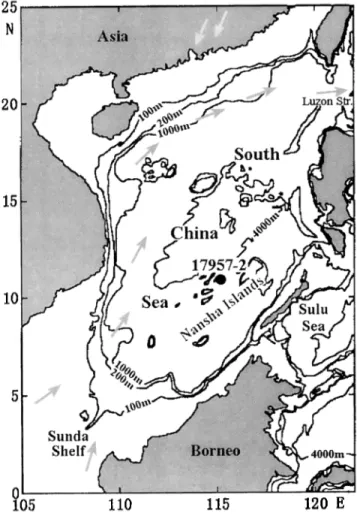
Figure 1. Location of core 17957-2 in the South China Sea. Gray arrows show modem surface currents during summer; white arrows show winter

monsoon.

Table 1. Sample Information of Core 17957-2 Used in This Study

Analytical Item Sample Interval, cm Number of Samples

Planktonic foraminifera 5 272 Benthic foraminifera 10 136 Calcareous nannofossil 20 51 Radiolarian 10 136 Stable isotope 10 138 Coarse fraction 5 273 Carbonate 10 139 Opal 5 272

2. Material and Methods

We studied gravity core 17957-2 raised from the southern SCS, north of the Nansha Islands (10ø53.9'N and 115ø18.3'E; water depth 2195 m; core length 1384 cm) (Figure 1) during the SONNE-95 cruise in 1994 [Sarnthein et al., 1994]. The sediment in the core consists of gray silty foraminiferal ooze free of turbiditic (or mass flow) deposition and major reworking. The core was sampled at 5-20-cm intervals, according to individual analytical item (Table 1). Three to ten cubic centimeters of wet sediment were dried and weighed for each sample while coarse fraction content was obtained through wet sieving over a 63-pm screen. Planktonic and benthic foraminifera were picked only from the size fraction > 150 pm. When planktonic foraminifera were abundant, the sample was split using biseparation method to yield a subsample containing at least 300 specimens.

Planktonic and benthic foraminifera were identified and counted. Our taxonomy follows that of Parker [ 1962], B• [ 1977], and Kennett and Srinivasan [ 1983] for planktonic foraminifera and that of Barker [ 1960] and Loeblich and Tappen [ 1988] for benthic foraminifera. On the basis of the census data the relative abundance of each species was calculated and plotted against depth to illustrate the down-core distribution patterns. We estimated the SSTs using two different planktonic foraminiferal transfer functions. The standard errors of the linear transfer function FP-12E [Thompson, 1981] are 2.48øC for winter SST and 1.46øC for summer SST, while those of the SIMMAX-28 formula using modern analog technique [Pfiaumann and dian, 1999] are 1.27 ø and 0.45øC, respectively. For the first time we used the thermocline depth transfer function of Andreasen and Ravelo [ 1997], which was based on the spatial distribution of 189 core top planktonic foraminifera in the tropical Pacific, to quantitatively reconstruct the changes of DOT in the SCS during the Pleistocene glacial cycles. This transfer function has a standard error of 22 m and additional 5 m of error due to insufficient counts in the core top database [Andreasen and Ravelo, 1997]. As for the benthic foraminifera, a Q mode factor analysis was carried out using the program of Klovan and Imbrie [ 1971 ]. Only species with relative abundance >2% in at least two samples (48 species and species groups, see Table 3) were included in the factor analysis. Carbonate dissolution/preservation was evaluated using changes in planktonic foraminiferal fragmentation, benthic foraminiferal proportion (expressed as BF/(BF+PF)%, where BF and PF are benthic and planktonic foraminiferal abundance, respectively), and the percentage of agglutinated tests in benthic foraminiferal fauna. Fragmentation is expressed as fragmentation =

JIAN ET AL.: MAJOR PLEISTOCENE PALEOCEANOGRAPHIC CHANGES 231

(F/8)/(F/8+W)%, where F is the number of fragments and W is that of well-preserved planktonic foraminifera in the sample [Le and Shackleton, 1992]. Calcareous nannofossil and radiolarian were analyzed only for providing biostratigraphic controls in this study and will be discussed in separate papers later.

Determination of carbonate content in the sample was made at Taiwan University according to the weight loss method outlined by Molnia [ 1974]. The salt in each sample was, however, washed out by distilled water before the carbonate material was dissolved by 1 N hydrochloric acid. Opal content was measured at Sun Yat-Sen University in Kaohsiung following the technique of Mortlock and Froelich [ 1989] with slight modifications described by Murray et al. [ 1993], except that 0.5 N NaOH instead of 2 M Na2CO3 was used to extract the biogenic opal. Overall, the analytical precision of the carbonate and opal determination are better than 1.0 and 1.5%, respectively.

Oxygen and carbon stable isotope measurements were carried out on the planktonic foraminiferal species Globigerinoides sacculifer (wo) (without a saclike final chamber) (>150 •tm) using a V. G. Micromass 602 mass spectrometer at the Institute of Earth Sciences, Academia Sinica at Taipei. The analytical precision expressed as 1 o for NBS-19 standard carbonate was 0.06%o. The average difference of duplicate foraminiferal analyses is-0.12%o for oxygen and 0.09?/00 for carbon.

High-resolution continuous paleomagnetic measurements were performed at the Laboratoire des Sciences du Climat et de 1' Environment (LSCE) of the Centre National de la Recherche Scientifique (CNRS)-Commissariat/• 1' Energie Atomique (CEA), France. The sediments were sampled using the 1-m-long u channel plastic container [Tauxe et al., 1983; Weeks et al., 1993]. The natural remnant magnetization was measured continuously with a resolution of-3 cm using a pass-through DC-SQUID cryogenic magnetometer in a shielded room. Stepwise in-line demagnetization with an average of 8-10 steps up to 60 mT was used to retrieve the primary component of the magnetization, which was isolated after the very first steps of demagnetization.

For spectral analyses a menu-driven PC program SPECTRUM [Schulz and Stattegger, 1997] was used. Compared to the widely used Blackman-Turkey approach for spectral analysis, the advantage of SPECTRUM is the avoidance of any interpolation of the time series. The interpolation of unevenly spaced time series may significantly bias statistical results because the interpolated

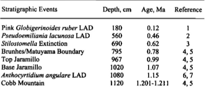
Table 2. Microfossil Datums and Magnetostratigraphic Events Adopted in This Study

Stratigraphic Events Depth, cm Age, Ma Reference Pink Globigerinoides ruber LAD 180 0.12 1

Pseudoemiliania lacunosa LAD 560 0.46 2 Stilostomella Extinction 690 0.62 3

Brunhes/Matuyama Boundary 795 0.78 4, 5 Top Jaramillo 967 0.99 4, 5 Base Jaramillo 1020 1.07 4, 5 Anthocyrtidium angulare LAD 1080 1.15 6, 7 Cobb Mountain 1120 1.201-1.211 4, 5

LAD is last appearance datum. (1) Thompson et al. [1979]; (2)

Thierstein et al. [1977]; (3) Sch6nfeld [1996]; (4) Shackleton et al. [1990]; (5) Berggren et al. [1995]; (6) Moore [1995]; (7) Shackleton et al. [1995].

data points are no longer independent [Schulz and Stattegger, 1997]. In this study, we selected 1.0 and 4.0 for the highest frequency factor (HIFAC) and the oversampling factor (OFAC), respectively, for a good compromise between computing time and smoothness of a spectrum. The time series was divided into three 50% overlapping Welch-overlapped-segment-averaging (WOSA) segments which were linearly detrended.

The material used in this study is stored at the Laboratory of Marine Geology, Tongji University. The complete data discussed

in this

paper

are

available

upon

request.

1

3. Results

3.1. Chronological Framework

First, a low-resolution chronological framework was developed on the basis of microfossil biostratigraphy and magnetostratigraphy for the last 1500 kyr. Four datums of calcareous and siliceous microfossils, including planktonic and benthic foraminifera, calcareous nannofossil, and radiolarian, were adopted in this study (Table 2). The Brunhes/Matuyama (B/M) magnetic polarity reversal (0.78 Ma) is clearly apparent as a change to negative inclination and a 180 swing of the declination at a depth of 795 cm. The upper Jaramillo (0.99 Ma) transition, unfortunately coinciding with the separation between two u channels, is around 967 cm. The lower Jaramillo (1.07 Ma) transition is situated at a depth of 1020 cm, again characterized by a change to negative inclination and a declination swing. The sharp swing in declination at 1120 cm might correspond to the Cobb Mountain event (between 1.201 and 1.211 Ma) (Figures 2 and 3 and Table 2).

Of particular interest is the discovery of microtekrites at the depths of 780-815 cm, with conspicuous peak at the depths of 805-810 cm slightly below the B/M boundary (Figure 3) [Zhao et al., 1999]. According to its chemical and physical properties, the microtekrites in the core also occurred extensively in deep sediments of Australasian area [Glass, 1967; Srnit et al., 1991 ] and Chinese loess [Wu et al., 1992]. It therefore can serve as an additional stratigraphic marker in the SCS. Time-to-depth conversions (Figure 2) were performed by assuming __ constant sedimentation rates between the biostratigraphic and magnetostratigraphic control points (Table 2), which shows no obvious hiatus in the core during the last 1500 kyr. The estimated

average sedimentation rate for the core is -0.93 cm/kyr.

We constructed more detailed age model primarily based on

foraminiferal 8180 and coarse fraction records, with constraints of

biostratigraphic and magnetostratigraphic control points (Figure 3).

The chronology for the isotopic age model was developed from

ODP Site 677 [Shackleton et al., 1990], different from those

proposed by Ruddirnan et al. [ 1989]. Coarse fraction stratigraphy

developed in the equatorial Indian Ocean [Bassinot et al., 1994]

• Supporting data are available on diskette or via Anonymous FTP from

www.agu.org, directly APEND (username = anonymous, Password =

guest). Diskette may be ordered from American Geophysical Union, 2000 Florida Avenue, N.W., Washington, DC 20009 or by phone at 800-966- 2481; $15.00. Payment must accompany order.

232 JIAN ET AL.: MAJOR PLEISTOCENE PALEOCEANOGRAPHIC CHANGES

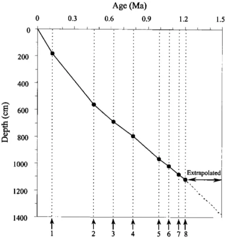
Age (Ma)

200 •

'

: :

_

rapolat•

1400--'

Figure 2. Age-depth plot showing sedimentation rates in core 17957-2: 1, pink Globigerinoides ruber last appearance datum (LAD); 2, Pseudoemiliania lacunosa LAD; 3, Stilostomella extinction; 4, Brunhes/Matuyama boundary; 5, top of Jaramillo; 6, base of

Jaramillo; 7, Anthocyrtidiurn angulare LAD; 8, Cobb Mountain event.

was applied in the SCS. Major peaks (CF2--,23) of the coarse fraction curve in core 17957-2 have been labeled according to their

position

relative

to the

b180

stratigraphy

(Figure

3), which

can

be

well correlated with those from ODP Site 758 in the Indian Ocean.

The age of each sample was interpolated on the basis of the average sedimentation rate between the isotopic age model control points. The base of the core reaches---1.50 Ma.

The

most

striking

change

for b•80

and

coarse

fraction

curves

is

3.2. Variations in the Sea Surface Temperature

Variations in the relative abundance of main planktonic foraminiferal species which could be divided into shallow- and

deep-dwelling species [B•, 1977; Fairbanks et al., 1982; Ravelo et al., 1990] were examined (Figures 4 and 5). MISs 22-20 from the MPR to B/M boundary and MISs 6-5 are two important boundaries. During MISs 6-5 the abundances of tropical-subtropical species Globigerinoides tuber and G. sacculifer (wo) remarkably decreased, while those of temperate species Neogloboquadrina dutertrei and Globorotalia crassaformis reached maximum, indicating a considerable decrease in SSTs. After MISs 22-20, the abundances of shallow-dwelling species G. ruber, G. sacculifer (wo) and Globigerina bulloides decreased, while those of deep-dwelling species Pulleniatina obliquiloculata, Globorotalia menardii, G. crassaformis, and Globorotalia infiata remarkably increased. Nevertheless, all the species in Figures 4 and 5 except G. infiata have no clear consistent glacial-interglacial changes.

Planktonic foraminifera in the core are well preserved with low fragmentation (<10%; see Figure 9), and the estimated SSTs using

two different

techniques

have

very

low correlation

(R2<0.01)

with

JIAN ET AL.' MAJOR PLEISTOCENE PALEOCEANOGRAPHIC CHANGES 233

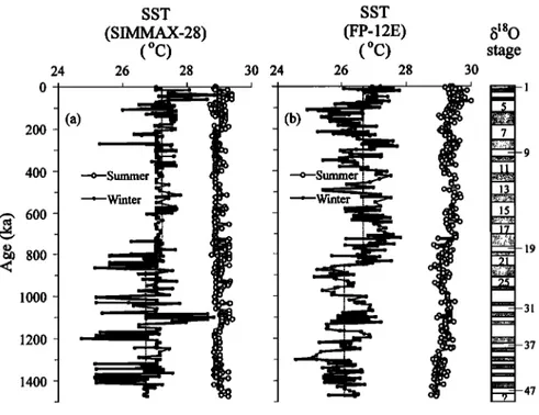
The estimated SSTs of core top from FP- 12E and SIMMAX-28 are 27.2 ø and 27.0øC for winter, and 29.4 ø and 28.9øC for summer, respectively. Their differences with the present day SSTs at this site (27.03øC for winter and 28.85øC for summer [Levitus and Boyer, 1994]) are less than the standard errors of estimation [Thompson, 1981; Pflaumann and Jian, 1999]. The SIMMAX-28-derived winter SST ranges from 24.7 ø to 27.8øC, averaging 27.0øC, while the SIMMAX-28-derived summer SST changes little from 28.8 ø to 29.4øC with an average of 29.0øC (Figure 6a). Their amplitudes of fluctuation are much greater than the standard errors of SIMMAX-28, indicating the changes of SIMMAX-28-derived SSTs are quite reliable. As for the FP- 12E-derived SSTs, the winter SST ranges from 24.5 ø to 27.8øC, averaging 26.4øC, while the summer SST changes little from 28.7 ø to 30.0øC with an average of 29.3øC (Figure 6b). The amplitude of fluctuation in the FP-12E-derived winter SST (3.3øC) is greater than the standard error of the FP-12E cold equation, implying that the changes of FP-12E-derived winter SST are really significant. Compared to previous data in the SCS using the transfer function FP-12E [Wang and Wang, 1990; Miao et al., 1994; Wang et al., 1995], both the estimated winter and summer SSTs from FP-12E and SIMMAX-28 are slightly warmer with a narrower range of seasonality in core 17957-2. This may be explained by the

fact that (1) the core is located in the tropical SCS as a part of WPWP and (2) it is far away from the influence of coastal currents. As shown in Figure 6a, the SIMMAX-28-derived winter SST changed little after the B/M boundary, except the excursions at MISs 7/8 and during MISs 6-5. However, before the boundary, it was very changeable with four distinct decreases. The average SIMMAX-28-derived winter SST before the B/M boundary is 26.7øC, lower than the average value of 27.2øC after it. However, the greatest change in the FP-12E-derived winter SST occurred at MISs 21/22, which divides the curve into two clear sections. The average FP-12E-derived winter SST was 26.6øC after MIS 21, while it was only 26.1 øC before the time (Figure 6b). on the basis of the results from two different transfer functions the tropical SSTs slightly increased right after the obvious decrease in winter SST during MISs 22-20, which may correspond to the climate changes at the MPR [Berger et al., 1993]. Since the B/M boundary, the winter SST changed within a range of <3øC, in agreement with those of Climate: Long-Range Investigation, Mapping, and Prediction (CLIMAP) Project Members [1981] in the western equatorial Pacific. This further supports that "the last 1.0 Ma was dominantly a period of lower SST in the late Neogene, except at the tropics where SST was a little higher than before and experienced only minor fluctuations in the western Pacific,"

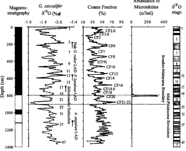
Magneto- G. sacculi•r

stratigraphy 8•80

(%o}

Coarse

Fraction

Microtektites 8• 80

(%)

(n/3ml)

stage

Figure 3. Magnetostratigraphic, oxygen isotopic, and coarse fraction stratigraphic framework in core 17957-2. The magnetostratigraphy is shown as a column with the usual black and white convention for normal and reverse periods, respectively.

Major peaks of the coarse fraction curve (CF2-•23) have been labeled according to their position relative to the 8•SO stratigraphy

[Bassinot et al., 1994]. The biostratigraphic and microtektite control points are also shown. Marine oxygen isotopic stages are indicated on the right side.

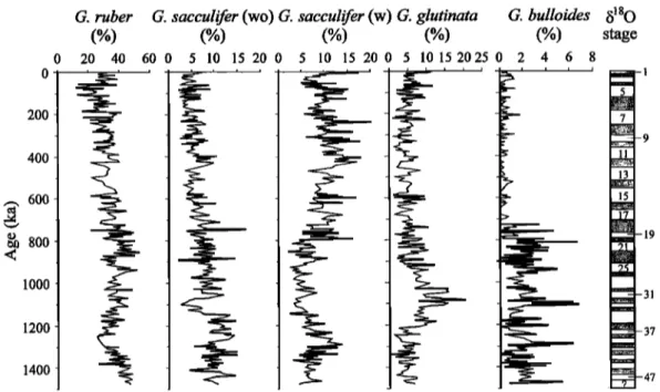
234 JIAN ET AL.' MAJOR PLEISTOCENE PALEOCEANOGRAPHIC CHANGES 200 400 600 800 1000 1200 1400 G. tuber (%) 20 40

G. sacculifer

(wo) G. sacculifer

(w) G. glutinata G. bulloides

b180

(%)

(%)

(%)

(%)

stage

60 0 5 10 15 20 0 5 10 15 20 0 5 10 15 2025 0 2 4 6 8

i • , !

Figure 4. Variations in relative abundance of selected shallow-dwelling planktonic foraminiferal species. G. sacculifer (w) is G. sacculifer with a saclike final chamber. Marine oxygen isotopic stages are indicated on the right side.

concluded by Wang [1994, p. 379]. It seems that the WPWP was relatively stable during the late Pleistocene glacial cycles [Thunell et al., 1994]. However, there was an obvious decrease in the winter SST during MISs 6-5, judging from the FP-12E-derived and SIMMAX-28-derived curves (Figure 6). This event made the winter SST higher during MISs 4-2 than during MIS 5, apparently conflicting with the pattern of glacial decrease and interglacial increase in SSTs revealed by previous studies in the SCS [Wang and Wang, 1990; Miao et al., 1994; Wang et al., 1995]. Therefore the SSTs here did not systematically vary with glacial-interglacial cycle.

3.3. Reconstruction of the Depth of Thermocline

Numerous tropical ocean studies suggest planktonic foraminiferal species abundance are controlled by upper water temperature and nutrient gradients [Fairbanks and Wiebe, 1980; Fairbanks et al., 1982; Bd et al., 1985; Ravelo et al., 1990; Martinetz, 1994; Andreasen and Rave]o, 1997]. Some researchers have investigated the potential usefulness of very deep dwelling species G. truncatulinoides for reconstruction of the upper thermal structure. This species has an unusual life cycle in that it reproduces at -600 m and from this depth, juveniles rapidly travel to the surface then slowly sink through the water column, growing by adding chambers [Bd, 1977; Bd et al., 1985; Hemleben et al.,

1989]. For this reason, a higher proportion of this species may indicated a very deep thermocline and/or thick mode water thermostads [Lohmann and Schweitzer, 1990; Lohmann, 1992; Ravelo and Fairbanks, 1992; Martinez, 1994, 1997]. The percentage abundance of G. truncatulinoides in core 17957-2 (Figure 7) show a trend of gradual decrease during the Brunhes chronozone which indicates the scale of mixing and the DOT have

gradually decreased. Especially, G. truncatulinoides left-coiling form, which requires a thermocline much deeper than right-coiling form, and Globoquadrina conglomerata (lives predominantly below 100 m as adults; [B•, 1977]) abruptly increased in MIS 5 (Figure 7), indicating that the thermal structure of upper water column greatly changed during the time interval.

The average estimated DOT of Holocene (-190 m) agrees with the modem annual DOT derived from the world ocean atlas of Levitus and Boyer [1994] in this region. Moreover, the average communality is 0.88, indicating this transfer function technique can interpret 94% of the total variance in the observed faunal information. The estimated DOT ranges from 115 to 230 m in the core, averaging 190 m. Generally, the DOT was relatively deeper during interglacial periods than during glacial periods. The most conspicuous change for the DOT was that it changed little around

200 m before MISs 22-21, that is, before the MPR, and then it

gradually decreased during the Brunhes chronozone, with an average of 180 m (Figure 7). The shallowest DOT (-115 m) occurred within MIS 6 and then became deep again after the abrupt increase of G. truncatulinoides left-coiling form and G. conglomerata in MIS 5.

Previous studies have revealed that when the DOT shoals, the mixed layer-dwelling species (G. ruber, G. sacculifer, and Globigerinita glutinata) decrease, while the thermocline-dwelling species (P. obliquiloculata, G. menardii, G. infiata, and N. dutertrei) increase in abundance [Ravelo et al., 1990; Ravelo and Fairbanks, 1992]. In core 17957-2 the MPR served as a turning point for the abundances of the mixed layer- and thermocline-dwelling species. The mixed layer-dwelling species decreased in abundance since the MPR and reached minimum during MISs 6-5, while the thermocline-dwelling species changed in an opposite trend (Figure 7), corresponding to the variations of the DOT. In fact, the shallowing of the DOT since the MPR was found also in the western equatorial Pacific [Schmidt et al., 1993].

JIAN ET AL.: MAJOR PLEISTOCENE PALEOCEANOGRAPHIC CHANGES 235 200 400 600

800

P. obliquiloculata

G. menardii Neogloboquadrina

G. crassaformis

G. infiata

(%) (%) 0 5 10 15 20 0 5 10 15 20 0 spp. (%) (%) (%) 10 20 30 0 2 4 6 8 0 2 4 stage 6

Figure 5. Variations in relative abundance of selected deep-dwelling planktonic foraminiferal species. Marine oxygen isotopic

stages are indicated on the right side.

After a minimum

shortly

before

the B/M boundary,

the b•80

3.4. Changes of Deep Water Masses

Deep-sea benthic foraminifera has been widely used to reconstruct the late Pleistocene variations in deep water masses, carbonate dissolution, and surface productivity in the SCS for the past few years [Miao and Thunell, 1996; Jian and Wang, 1997;

24 0 200 400 •, 600 • 800 100o 1200 1400 (a) SST (SIMMAX-28)

(øc)

(øC)

15180

Figure 6. Down-core variations in the (a) SIMMAX-28-derived and (b) FP-12E-derived winter and summer SSTs. Dashed lines show the average winter SST: before and after the B/M boundary (Figure 6a) and before and after MIS 21 (Figure 6b). Marine

236 dIAN ET AL.' MAJOR PLEISTOCENE PALEOCEANOGRAPHIC CHANGES

Mixed layer-

Depth of thermocline Dwelling (m) Species (%) 100 150 200 250 30 45 60 75 5 0 200 400 6OO 800 lOOO 12oo 14oo Thermocline-

Dwelling G. truncatulinoides G. truncatulinoides G. conglornerata 15•aO

Species (%) (right-coiling) (%) (left-coiling) (%) (%) stage

20 35 500 2 4 6 810 0 2 4 6 8 0 2 4 6 8

i ,!

' ' 1

Figure 7. Long-term changes in the DOT estimated using transfer function of Andreasen and Ravelo [ 1997], relative abundances of mixed layer-dwelling species (Globigerinoides tuber, Globigerinoides sacculifer, and Globigerinita glutinata), thermocline-dwelling species (Pulleniatina obliquiloculata, Globorotalia menardii, Globorotalia infiata, and Neogloboquadrina dutertrei), right-coiling and left-coiling Globorotalia truncatulinoides, and Globoquadrina conglomerata. Dashed lines show the general trends of change before and after MISs 22-21. Marine oxygen isotopic stages are indicated on the right side.

Kuhnt et al., 1999]. dian et al. [1999] recently claimed that deep-sea benthic foraminifera in the SCS might be divided into two major groups whose distributions are primarily controlled by the organic flux to the seafloor and the chemical/physical

properties in the ambient water mass, respectively. Therefore

benthic foraminiferal species and assemblages could be used to monitor the general trend of changes in deep water masses during the Pleistocene in the SCS [dian and Wang, 1997].

Abundance G. subglobosa A. novozealandicum E. bradyi Stilostomella G. molluscensis P bulloides

(n/cm 3) (%) (%) (%) (%) (%) (%) 0 3060901200102030400 15 30 450 5101520250 5101520250 15 30 450 510152025

o

Figure 8. Variations in the abundance of benthic foraminiferal fauna and percentage abundance of main benthic foraminiferal

dIAN ET AL.: MAJOR PLEISTOCENE PALEOCEANOGRAPHIC CHANGES 237 The abundance of benthic foraminiferal fauna (number of

specimens per cubic centimeter) varies between 10 and 110 in the core, with lower values prior to the B/M boundary (Figure 8), implying a great change in deep water conditions at that time. On

the basis of the down-core distribution of main benthic

foraminiferal species (Figure 8), two important boundaries are

found at the B/M boundary and MIS 5. At the B/M boundary,

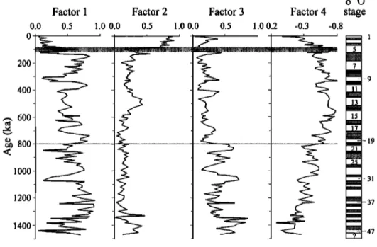
Pullenia bulloides increased significantly in abundance, while Stilostomella spp. remarkably decreased and then became extinct at the depth of 690 cm. Moreover, since MIS 5, Globocassidulina subglobosa obviously decreased in abundance, while Astrononion novozealandicum increased. We used Q mode factor analysis to better discriminate benthic foraminiferal assemblages. As a result, four varimax factors were obtained, which explain 78.6% of the total variance. According to the down-core variations in factor loadings of each factor (Figure 9) and the factor scores of each species or species groups (Table 3), factor 1, absolutely dominated by G. subglobosa, controls most part of the last 1500 kyr before MIS 5. However, factor 2, represented by the A. novozealandicum assemblage which is characteristic of A. novozealandicum and Eggerella bradyi (Figure 8), became more important since MIS 5. Factor 3, dominated by Stilostomella spp. and Globocassidulina molluscensis, was important before the B/M boundary, especially toward the bottom of the core, while factor 4, represented by the P. bulloides assemblage, controlled the period between the B/M boundary and MIS 5.

G. subglobosa is the dominant species of the modem Intermediate Water Mass (IWM) in the SCS as resolved by the same technique [dian and Wang, 1997]. Because factor 1 is characterized by this species, its variations in factor loading should represent the changes of the IWM. From Figure 9 it is inferred that core 17957-2 is bathed in the Deep Water Mass (DWM) now, but it

was mainly controlled by the IWM before MIS 5. The remarkable decease in factor 1 and the relative abundance of G. subglobosa since MIS 5 indicate that the IWM weakened, as revealed by a previous study [dian and Wang, 1997]. Particularly, the IWM displays a general trend of glacial decrease and interglacial increase, which is obviously superimposed by long-term fluctuations of-200 kyr.

Compared with those of the IWM, the changes of the DWM are much more complicated. A. novozealandicurn is the dominant species of the modem DWM in the SCS, especially in the oligotrophic area [dian and Wang, 1997]. The remarkable increase in factor 2 and the relative abundance of this species since MIS 5 indicated that the DWM abruptly strengthened at the expense of the IMW. Before that time, P. bulloides assemblage of factor 3 and Stilostomella spp. assemblage of factor 4 had successively represented the DWM instead ofA. novozealandicurn assemblage (Figure 9) because P. bulloides is one of the characteristic species of the modem DWM [dian and Wang, 1997], while Stilostomella spp. is commonly found in cores with present water depths between 1500 and 3000 m [SchOnfeld, 1996]. The faunal turnovers indicate that there were two major changes in the DWM over the last 1500 kyr. The first one occurred at the B/M boundary, slightly later than the changes in SSTs and DOT. The second one took place within MIS 5, possibly corresponding to the major changes in surface productivity (see Figure 11) and/or the thermal structure of upper water column (Figure 7) at that time.

3.5. Deep-Sea Carbonate Dissolution Fluctuations

The percentage of agglutinated tests in benthic foraminiferal fauna, BF/(BF+PF)% , and relative abundance of agglutinated E.

Factor 1 Factor 2 0.0 0.5 1.0 0.0 0.5 0 200 400 600 800 1000 1200 1400 1.0 0.0 Factor 3 Factor 4 0.5 1.0 0.2 -0.3

•18

O

Figure 9. Results of Q mode factor analysis on benthic foraminifera, showing down-core variations in factor loading of the four varimax factors. The most important boundaries at the B/M boundary and MIS 5, respectively, are shaded. Marine oxygen isotopic

238 dIAN ET AL.: MAJOR PLEISTOCENE PALEOCEANOGRAPHIC CHANGES Table 3. Matrix of Factor Scores of the Four Benthic

Foraminiferal Q mode Varimax Factors

Species / Species Groups Factor 1 Factor 2 Factor 3 Factor 4

Eggerella bradyi -0.089 0.314 -0.087 -0.386 Sigmoilopsis schlumbergeri 0.010 -0.008 0.031 -0.002 Pyrgo spp. -0.009 -0.011 0.218 -0.077 Triloculina tricarinata -0.020 -0.012 0.198 -0.042 Quinqueloculina seminula 0.015 0.017 0.218 -0.086 Quinqueloculina venusta -0.009 -0.008 0.039 -0.034 Quinqueloculina spp. 0.003 0.005 0.054 0.006 Lagena spp. 0.020 0.044 0.115 -0.042 Fissurina spp. 0.092 0.109 0.279 -0.203 Nodosaria spp. 0.012 -0.002 0.047 0.013 Dentalina spp. 0.050 0.022 0.131 0.042 Stilostomella spp. 0.087 -0.113 0.639 0.186 Guttulina spp. 0.006 0.039 0.020 -0.037 Bolivina pacific -0.024 -0.020 0.074 -0.027 Pleurostornella alternans 0.051 -0.012 0.102 0.044 Bulimina alazanensis -0.013 -0.030 -0.041 -0,•244 Bulimina aculeata -0.077 0.016 0.034 -0.144 Uvigerina peregrina -0.003 -0.004 0.026 -0.099 Uvigerina auberiana -0.033 0.112 0.057 -0.050 Reussella spinulosa -0.010 0.043 0.008 0.000 Francesita advena -0.001 0.026 0.029 -0.020 Ehrenbergina undulata 0.101 0.031 0.052 0.099 Cassidulina crassa 0.002 0.006 0.006 -0.017 Cassidulina laevigata 0.003 0.137 -0.024 -0.029 Rutherfordoides tenuis -0.019 -0.008 0.154 0.012 Globocassidulina subglobosa 0.961 -0.032 -0.095 -0.098 Globocassidulina molluscensis 0.006 0.255 0.371 0.108 Favocassidulinafavus -0.006 -0.014 0.045 -0.119 Pullenia bulloides -0.050 -0.056 -0.067 -0.596 Pullenia quinqueloba -0.055 0.053 0.190 -0.171 Melonis barleeanum 0.049 0.077 0.013 -0.047 Melonis pompilioides 0.056 -0.021 -0.025 -0.075 Astrononion novozealandicum 0.019 0.798 -0.084 0.209 Elphidium spp. -0.014 0.023 0.016 -0.008 Epistominella exigua -0.018 -0.031 0.036 -0.095 Sphaeroidina bulloides -0.004 0.066 0.033 -0.095 Anomalina globulosa 0.007 -0.005 0.051 -0.049 Hoeglundina elegans -0.009 0.052 0.006 -0.003 Oridosalia umbonatus 0.055 0.132 0.116 -0.184 Gyroidina orbicularis -0.013 0.031 -0.003 -0.060 Gyroidinoides lamarckiana 0.006 0.091 0.057 -0.262 Osangularia culter -0.018 -0.007 0.085 -0.048 Cibicidoides robertsonJanus 0.106 0.284 0.016 -0.041 Cibicidoides cf. robertsonJanus 0.000 -0.019 0.064 -0.015 Cibicidoides wuellerstorfi -0.028 -0.051 0.207 -0.212 Cibicidoides kullenbergi 0.015 -0.017 0.091 -0.008 Cibicides sp. 0.011 -0.016 0.022 -0.017 Cibicides okinawaensis 0.003 -0.010 0.018 -0.010

bradyi can be used to evaluate deep-sea carbonate dissolution [Bian et al., 1992; Miao and Thunell, 1996]. Their obvious increases during the Brunhes chronozone show strengthened dissolution (Figures 8 and 10). In fact, planktonic foraminiferal fragmentation is the best indicator for deep-sea carbonate dissolution [Le and Shackleton, 1992; Miao et al., 1994], with high values related to enhanced dissolution. In core 17957-2 the fragmentation curve is negatively well correlated with the coarse fraction and carbonate curves (Figure 10). They display a distinct glacial-interglacial pattern since the MPR. The dissolution spikes with high fragmentation and low coarse fraction and carbonate always occurred in the interglacial stage and the transition from

interglacial to glacial stage, for example, MISs 5, 6/7, 8/9, 11, 12/13, 14/15, 17, 18/19, and 21. These spikes can be recognized to correspond to the dissolution events of B3, B5, B7, B9, B11, B13, B15, B17, and M1 in the equatorial Pacific, respectively [Farrell and Prell, 1989, 1991 ]. This typical "Pacific-type" carbonate cycle [Thunell et al., 1992; Wang et al., 1995] in the core further confirms that the SCS shared the same carbonate dissolution signals as the tropical Pacific during the Pleistocene [Farrell and Prell, 1989, 1991; Yasuda et al., 1993].

However, the glacial-interglacial pattern of fragmentation is superimposed by a long-term oscillation with an irregular cycle length. Maxima in the fragmentation curve are found at the MPR, MISs 13-11 and MIS 5, in agreement with the changes in the percentage of agglutinated benthie foraminifera and BF/(BF+PF)% (Figure 10). This long-term oscillation of carbonate dissolution has been found in the tropical Pacific and Indian Ocean [Vincent, 1981; Bassinot et al., 1994]. Among the three periods of enhanced dissolution, the recent one possibly corresponded to the great changes in planktonic and benthie foraminiferal fauna during MISs 6-5 (Figures 4-9). The middle one centered at-400 ka is known as the "middle Brunhes dissolution event" [Farrell and Prell, 1989; Bassinot et al., 1994]. The lower one at the MPR is not the most striking, though with the highest fragmentation which is not supported by other dissolution indices. Compared to those before the MPR, the average values of fragmentation, percentage of agglutinated benthie foraminifera and BF/(BF+PF)% were higher, while that of coarse fraction and carbonate were lower after the MPR (Figure 10). This implies slightly increased carbonate dissolution as a whole after the MPR in the southern SCS.

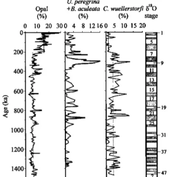
3.6. Enhanced Surface Productivity Over the Last 200 kyr Now it is more than apparent that abundance and species composition of benthic foraminifera are primarily controlled by the organic carbon flux to the seafloor and thus, ultimately, by the surface productivity [Herguera and Berger, 1991; Sarnthein and Altenbach, 1995; Miao and Thunell, 1996; dian et al., 1999; Kuhnt et al., 1999]. It has been found that benthic foraminifera Bulimina aculeata and Uvigerina peregrina are well associated with high surface productivity in the SCS [Miao and Thunell, 1996; dian et al., 1999]. Their relative abundances are generally <5% in the core (Figure 11), indicating a very low surface productivity at this site, which is consistent with the modem distribution of surface primary productivity in the SCS [The Multidisciplinary Oceanographic Expedition Team, 1992]. Nevertheless, the relative abundance of B. aculeata and U. peregrina generally increased during glacial periods, especially in MISs 22, 8, and 6, indicating that the productivity slightly increased at these times.

Biogenic opal is a parameter related to the surface productivity [Herguera and Berger, 1991; Murray et al., 1993 ]. The percentage of opal in the core ranges from 2.7 to 28.3%, with an important

boundary

at-200 ka around

MISs 6/7. The average

vdlue

of opal

JIAN ET AL.' MAJOR PLEISTOCENE PALEOCEANOGRAPHIC CHANGES 239 200 400 600 800, 1000, 1200' 1400'

CaCO3 Coarse

fraction

b'So

(%) (%) stage 40 50 60 70 80 90 0 20 40 60 80 0 2 Fragmentation Agglutinants BF/(BF+PF) (%) (%) (%) 5 10 0 10 20 30 0 1 i B3

,•[ B13

•B15 _

Figure 10. Deep-sea carbonate dissolution indices versus depth. B3-17 and M1 indicate major spikes of the fragmentation curve according to their corresponding dissolution events in the equatorial Pacific [Farrell and Prell, 1989, 1991 ]. Dashed lines show the average values before and after the MPR, respectively. Marine oxygen isotopic stages are indicated on the right side.

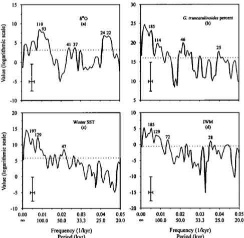
3.7. Periodic Variations in Paleoceanographic Records

Spectral analysis was used to study the variability of four

paleoceanographic

records

(b•80, G. truncatulinoides

percent,

FP-12E-derived winter SST, and IWM) for the last 1500 kyr (Figure 12). The IMW is represented by the factor loadings of

benthic foraminiferal factor 1 as above discussed. After

SPECTRUM has performed the analysis, some statistical

0 200 400 600 800 1000' 1200 1400 0 U. peregrina

Opal

+B.

aculeata

C. wuellerstorfi

b•SO

Figure 11. Down-core variations in the surface paleoproductivity indices. Dashed lines show the average values before and after 200 ka, respectively. Marine oxygen isotopic stages are indicated on the right side.

parameters are displayed. Probably the most important is the reliable frequency range. Assuming that at least two full cycles are observed within each WOSA segment, the lowest reliable frequency in this study is 0.0027 1/kyr, corresponding to the period of 370 kyr. The spectral peaks with lower frequency than this limit are discarded in the study.

According

to Figure 12a, the b•80 record

reveals

clear

the IWM record,

in contrast

to the spectrum

of the b•80 record.

frequency

pa,

leoceanographic

oscillations

in three

dimensions

of

240 JIAN ET AL.' MAJOR PLEISTOCENE PALEOCEANOGRAPHIC CHANGES 15 3 $"0 G. truncatulinoides percent •, 10 i 10 (a) 2 185 (b)

-

ß

• 5

2

i14 46

• 0

1

0.00 0.01 0.02 0.•)3 0.04 0.05

0.05

AAi2

9

(d)

0.00 0.•)1 0.•2 0.03 0.04

Figure 12.' Spectral analysis of four paleoceanographic records: (a) 15•SO, (b) Globorotalia truncatulinoides percent, (c) winter SST estimated using FPo12E transfer function, and (d) IWM for the last 1500 kyr (Settings: OFAC = 4.0; HIFAC = 1.0; number of

segments is three; Welch window except Hanning window for 15•SO: See Schulz and Stattegger [1997] for detailed description of

these parameters). Numbers above peaks denote respective periods. Cross in lower left comer marks 6odB bandwidth (horizontal)

and 80% confidence interval (vertical). Horizontal dashed line denotes the average value of the spectrum and is a rough estimate for

a white noise component in the time series. Considering only those parts of spectral peaks above this level gives an estimation of

their corresponding variance contribution. 4. Discussion

Variations of the SSTs and DOT in the SCS are primarily a response to monsoonal wind-driven surface circulation [Wyrtki, 1961]. Core 17957-2 is located in the tropical SCS, where the foraminifera-based paleo-SST reconstruction has been a vigorous point of discussion in recent years [Pfiaumann and Jian, 1999]. In this study, we applied two different transfer functions SIMMAX-28 and FP-12E. Both results show that the SSTs here have no consistent glacial-interglacial changes. Though there is nearly no tendency of point-by-point comparable SSTs, both results reveal (1) the slightly increased SSTs as a whole right after MISs 22-20 and (2) the obviously decreased winter SST during

MISs 6-5.

Comparatively speaking, we have little knowledge about the variation of modem DOT in the SCS. Being a part of the WPWP, the southern SCS has other effects on its variation in the DOT except the East Asian monsoonal wind system. For example, the variations in the magnitude of the trade winds and associated equatorial currents may affect regional SCS circulation [Wyrtki,

1961 ]. Especially, during the Pleistocene glacial periods the SCS changed its configuration into a semienclosed basin due to the exposed shelf [Wang et al., 1995]. This caused the outflow of

subsurface water from the SCS into the Indian Ocean [Wyrtki, 1961] to be unlikely and altered the upper water structure of the southern SCS. The DOT there indeed experienced significant variations over the last 1500 kyr. Since the MPR, the DOT

gradually became shallower until MISs 6-5 and then deepened

afterward, as also confirmed by the changes in very deep dwelling

species G. truncatulinoides. The shallowest DOT in MIS 6 can be

used to evoke an upwelling enhancing the surface productivity. It is interesting that the two major changes in deep water masses of the southern SCS were almost synchronous with those in surface water masses but generally with a potential lag in response. For example, planktonic foraminiferal fauna responded to the MPR immediately, while benthic foraminiferal fauna did not change until the B/M boundary. As for the paleoceanographic

changes within MISs 6-5, the winter SSTs, DOT, and surface

productivity greatly changed since MIS 6, while the deep water masses changed since MIS 5. Therefore both the surface and deep circulation in the southern SCS had experienced significant variations over the last 1500 kyr.

A variety of interpretations have been suggested to explain the

striking paleoceanographic changes at the MPR, such as changes

in North Atlantic Deep Water production [Farrell and Prell, 1991 ], increase of marine-based ice sheets, uplift of highlands from erosion, and tectonic forces [Ruddiman and Rayrno, 1988; Berger