Estimating aerosol emissions by assimilating observed aerosol optical depth in a global aerosol model

(1)

HAL Id: hal-01111703

https://hal.archives-ouvertes.fr/hal-01111703

Submitted on 30 Jan 2015

HAL is a multi-disciplinary open access

archive for the deposit and dissemination of

sci-entific research documents, whether they are

pub-lished or not. The documents may come from

teaching and research institutions in France or

abroad, or from public or private research centers.

L’archive ouverte pluridisciplinaire HAL, est

destinée au dépôt et à la diffusion de documents

scientifiques de niveau recherche, publiés ou non,

émanant des établissements d’enseignement et de

recherche français ou étrangers, des laboratoires

publics ou privés.

aerosol optical depth in a global aerosol model

N. Huneeus, F. Chevallier, Olivier Boucher

To cite this version:

N. Huneeus, F. Chevallier, Olivier Boucher. Estimating aerosol emissions by assimilating observed

aerosol optical depth in a global aerosol model. Atmospheric Chemistry and Physics, European

Geosciences Union, 2012, 12 (10), pp.4585-4606. �10.5194/acp-12-4585-2012�. �hal-01111703�

(2)

Atmos. Chem. Phys., 12, 4585–4606, 2012 www.atmos-chem-phys.net/12/4585/2012/ doi:10.5194/acp-12-4585-2012

Atmospheric

Chemistry

and Physics

Estimating aerosol emissions by assimilating observed aerosol

optical depth in a global aerosol model

N. Huneeus1,*, F. Chevallier1, and O. Boucher2

1_{CNRS/INSU/Laboratoire des sciences du climat et de l’environnement (LSCE) – UMR8212, Gif-sur-Yvette, France} 2_{Laboratoire de M´et´eorologie Dynamique, IPSL, CNRS/UPMC, Paris, France}

*_{now at: Laboratoire de M´et´eorologie Dynamique, IPSL, CNRS/UPMC, Paris, France}

Correspondence to: N. Huneeus (nicolas.huneeus@lsce.ipsl.fr)

Received: 2 December 2011 – Published in Atmos. Chem. Phys. Discuss.: 27 January 2012 Revised: 12 April 2012 – Accepted: 18 April 2012 – Published: 24 May 2012

Abstract. This study estimates the emission fluxes of a range

of aerosol species and one aerosol precursor at the global scale. These fluxes are estimated by assimilating daily to-tal and fine mode aerosol optical depth (AOD) at 550 nm from the Moderate Resolution Imaging Spectroradiometer (MODIS) into a global aerosol model of intermediate com-plexity. Monthly emissions are fitted homogenously for each species over a set of predefined regions. The performance of the assimilation is evaluated by comparing the AOD af-ter assimilation against the MODIS observations and against independent observations. The system is effective in forc-ing the model towards the observations, for both total and fine mode AOD. Significant improvements for the root mean square error and correlation coefficient against both the as-similated and independent datasets are observed as well as a significant decrease in the mean bias against the assimi-lated observations. These improvements are larger over land than over ocean. The impact of the assimilation of fine mode AOD over ocean demonstrates potential for further improve-ment by including fine mode AOD observations over conti-nents. The Angstr¨om exponent is also improved in African, European and dusty stations. The estimated emission flux for black carbon is 15 Tg yr−1, 119 Tg yr−1 for particulate or-ganic matter, 17 Pg yr−1for sea salt, 83 TgS yr−1for SO2and

1383 Tg yr−1for desert dust. They represent a difference of +45 %, +40 %, +26 %, +13 % and −39 % respectively, with respect to the a priori values. The initial errors attributed to the emission fluxes are reduced for all estimated species.

1 Introduction

Accurate knowledge on the spatial and temporal distribution of aerosol emissions is needed to quantify their impact on cli-mate and air quality. Uncertainties in emissions contribute to the uncertainties associated with the aerosol radiative forcing (e.g., Forster et al., 2007). Many of the numerous studies that estimate the emissions of individual aerosol species focus on anthropogenic emissions while limited effort has been ded-icated to estimate the emissions of natural aerosols, such as desert dust (DD) and sea salt (SS) at the global scale.

Emissions of natural DD and SS aerosols are either pre-scribed in global models or interactively calculated as a func-tion of wind speed and other local variables. For instance DD emissions are usually parameterised as a function of soil properties such as soil particle size distribution, vegetation cover and soil moisture (e.g. Tegen et al., 2002). Actual mea-surements characterizing emission processes remain limited (e.g. Sow et al., 2009; Alfaro et al., 2004; Rajot et al., 2003; O’Dowd et al., 1997) and model emissions are therefore val-idated indirectly through assessment of the model perfor-mance in simulating atmospheric concentrations, surface de-position fluxes or aerosol optical depth (Ginoux et al., 2001; Tegen et al., 2002; Huneeus et al., 2011). Global models present a large diversity in simulating DD emissions mainly due to the different parameterisations and input data to these parameterisations whereas the diversity in SS emissions is mainly due to differences in the simulated particle size (Tex-tor et al., 2006).

For black carbon (BC), particulate organic matter (POM) and sulphate (SU) aerosols and/or their precursors, emissions

(3)

are prescribed using global inventories exclusively based on bottom-up techniques which integrate source information across different economical sectors. We observe a smaller di-versity among global models due to the use of similar data sets (Textor et al., 2006). For BC and POM some of the most commonly used inventories in global models are Cooke et al. (1999) and Bond et al. (2004). These inventories describe the aerosol fluxes based on emission factors relating the emit-ted amount to a particular economical sector. The inventory from the Emission Database for Global Atmospheric Re-search (EDGAR) presents fluxes for sulphur dioxide (SO2)

among other gases by country and sector based on emis-sion factors (Olivier et al., 2002). Dentener et al. (2006) pre-pared an emission inventory for primary aerosols and precur-sor gases by combining pre-existing inventories. Lamarque et al. (2010) document the new emission inventories which have been prepared for the Climate Model Intercomparison Program #5 (CMIP5) exercise.

Some emission estimates have been generated by com-bining existing bottom-up inventories with satellite data. Streets et al. (2003) used the Advanced Very High Res-olution Radiometer (AVHRR) fire count and Total Ozone Mapping Spectrometer (TOMS) aerosol index (AI) to in-troduce spatial and temporal variability in a bottom-up ap-proach to estimate biomass burning emissions in Asia. Gen-eroso et al. (2003) generated a new emission inventory of car-bonaceous aerosols by redistributing in space and time pre-existing estimates based on satellite fire products. Vermote et al. (2009) estimate global biomass burning emissions based on emission coefficients obtained from combining satellite derived fire radiative energy and existing emission estimates. Ito and Penner (2005) generated emission estimates for the year 2000 for biomass and fossil fuel burning by combining existing emission inventories and scaled them back in time based on TOMS AI till 1979 and on methane emission from Stern and Kaufmann (1996) beyond that.

In the last decade, top-down techniques have been de-veloped to estimate aerosol emission fluxes based on the combination of satellite data and numerical models. Hoelze-mann et al. (2004) estimated the wildland fire emissions for the year 2000 with the Global Wildland Fire Emission Model (GWEM) based on the burned area from the Global Burnt Scar satellite product (GLOBSCAR). An important technique for this purpose is data assimilation, which con-sists in estimating a statistically-optimal state by finding the best compromise between a priori (or first-guess) informa-tion and observainforma-tions. Zhang et al. (2005) estimated the biomass burning emissions for 1997 by assimilating TOMS AI. Hakami et al. (2005) used the variational data assimila-tion approach to estimate BC emissions and their initial con-dition over eastern Asia by assimilating concentration mea-surements. Yumimoto et al. (2007, 2008) applied the same approach to estimate dust emissions for dust events by as-similating lidar observations. Dubovik et al. (2008) estimated the emissions of fine and coarse mode aerosols for a period

of two weeks in August 2000 by assimilating Moderate Res-olution Imaging Spectroradiometer (MODIS) aerosol optical depth (AOD) at 550 nm in the GOCART aerosol model.

This is the first study to estimate simultaneously the global emissions for multiple aerosol species and one gaseous pre-cursor (namely DD, SS, BC, POM and SO2). These aerosol

fluxes are estimated in a consistent and coherent manner by assimilating daily total and fine mode AOD at 550 nm from MODIS into an aerosol model of intermediate complexity (Huneeus et al., 2009). We describe the data and methodol-ogy used to derive the emission estimates in Sect. 2. In Sect. 3 we present the results of the inversion both in terms of AOD and emission fluxes. In Sect. 4 the uncertainties of the esti-mated fluxes are discussed. Finally Sect. 5 presents the con-clusion of this work.

2 Data and methodology 2.1 Assimilation method

In this study, we seek statistically-optimal aerosol emission fluxes that represent the best compromise between the ob-servations y and the a priori information xb. We follow here and throughout the text the notation of Ide et al. (1997). In a Bayesian framework this optimal state vector xa, also known as analysis, is found by minimizing a scalar cost function J . This cost function is defined as the sum of the departures of a potential solution x and the corresponding simulated obser-vations to the a priori information xb_{and the given}

observa-tions y:

J (x) = 1/2(x − xb)TB−1(x − xb) +1/2(H (x) − y)TR−1(H (x) − y) (1) where H is the non-linear observation operator that computes the equivalent of the observations y for a given state vector x,

R is the covariance matrix of the error statistics of the

obser-vations and B is the covariance matrix of the error statistics of the a priori information.

Different approaches allow finding the minimum of the above cost function (e.g. Rodgers, 2000). In the linear case, the analysis xacan be computed through either analytical for-mulations

xa=xb−(HTR−1H + B−1)−1HTR−1(Hxb−y) (2) or

xa=xb−BHT(HBHT+R)−1(Hxb−y) (3) where H is the linear operator of H . It is possible to loop on Eqs. (2) and (3) to account for a non-linear operator.

Alternatively, one can use an equivalent variational for-mulation of the Bayesian estimation problem. In this case, the analysis xa is obtained by finding the minimum of the cost function in an iterative way through a descent algorithm

(4)

N. Huneeus et al.: Estimating aerosol emissions by assimilating observed aerosol optical depth 4587

(e.g., Chevallier et al., 2005). The descent direction is given at each iteration by the gradient of the cost function J with respect to the control variable x.

The methods described by Eqs. (2) and (3) and the vari-ational approach are equivalent and practical considerations determine the approach chosen to minimize the cost function J of Eq. (1) and obtain the analysis xa. The two analytical formulations (Eqs. 2 and 3) differ in the size of the matrix to be inverted. The relative size of the state vector and the mea-surement vector guide the choice of formulation. When the size of the state vector is small and R is easy to invert (e.g., R is diagonal), Eq. (2) is more appropriate. Conversely, Eq. (3) is more convenient if the size of R is small and all elements of H are directly known. In both approaches the analysis is computed based on the departures or differences between the simulated (Hxb) and observed (y) values, the sensitivities of the observation operator (H) and the relative weights of the

R and B matrix. At any given grid box, the difference

be-tween the model and observations (weighted by R and B) is reduced by adjusting the elements of the state vector pre-senting the highest sensitivity to the perturbations in that grid box. For cases with large state vector and observation vector, the variational approach is the most appropriate one. In the present study, we use Eq. (2) to minimize the cost function J in view of the size of our state vector (Sect. 2.3) and the way

R is defined (Sect. 2.5). The assumption of linearity in this

approach will be addressed in Sect. 2.6.

2.2 Observation operator

The observation operator used in this work is the simplified aerosol model (hereafter SPLA) which has been documented in Huneeus et al. (2009). This model computes the fine mode and total AOD at three wavelengths, 550, 670 and 865 nm. It was derived from the general circulation model of the Labo-ratoire de M´et´eorologie Dynamique (LMDZ) (Reddy et al., 2005). The SPLA model groups the 24 original tracers sim-ulated in LMDZ into 4 tracers, namely the gaseous precur-sors, the fine mode aerosols, the coarse sea salt aerosols and the coarse desert dust aerosols. The gaseous aerosol precur-sor groups together dimethylsulfide (DMS), sulphur dioxide (SO2) and hydrogen sulfide (H2S). The aerosol fine mode

includes sulphate (SU), black carbon (BC), particulate or-ganic matter (POM), desert dust (DD) with radius between 0.03 and 0.5 µm and sea salt (SS) aerosols with radii smaller than 0.5 µm. The SS coarse mode groups together the par-ticles with radii between 0.5 and 20 µm whereas the coarse DD mode corresponds to particles with radii between 0.5 and 10 µm. We keep the original emission configuration for each aerosol species and gaseous precursor. These emissions are grouped into the four tracers only after emission and are treated as such from that point on. Consequently with the re-duction in the number of tracers, new values of deposition velocities, mass median diameter and mass extinction effi-ciencies were recomputed according to the new tracers.

Fur-thermore, the sulphur chemistry was reduced to an oxidation mechanism as a function of latitude and no distinction be-tween hydrophilic and hydrophobic OM and BC was done. Both models are equivalent in all other aspects. The model is driven by 6-hourly reanalysis data from the European Centre for Medium-Range Weather Forecasts (ECMWF).

As shown by Huneeus et al. (2009), the SPLA model suc-cessfully reproduces the main features of the LMDZ aerosol burdens for each one of the aerosol species. The main dif-ferences between these models are on one hand caused by differences in the deposition and sedimentation fluxes asso-ciated to new deposition and sedimentation velocities and on the other hand caused by the simplification of the sulphur chemistry to a simple oxidation of sulphur to sulphate. The largest differences in AOD in terms of monthly mean, with both LMDZ and AERONET, are observed over sites with strong DD influence. The model has a better performance in reproducing the monthly variability of AOD in LMDZ than the daily one. When comparing to AERONET daily AOD, SPLA reproduces the baseline but has difficulties in repro-ducing the daily variability associated with episodic changes in the aerosol load. In this case the largest differences are observed in stations dominated by industrial aerosols.

The first-guess or a priori aerosol emission fluxes used in the inversion system are the ones used in Reddy et al. (2005). The sulphur emissions from fossil fuel combus-tion and industrial processes are taken from the EDGAR ver-sion 3.0 database (Olivier and Berdowski, 2001), from which a fixed 5 % from combustion sources is assumed to be emit-ted directly as sulphate. For the natural emissions we take the same sulphur emissions as those described in Boucher et al. (2002). Organic carbon (OC) is always associated with oxygen, hydrogen and other chemical species and the result-ing aerosol is called particulate organic matter (POM). This POM emissions are derived from the organic carbon (OC) ones considering a conversion rate of 1.4 and 1.6 for fos-sil fuel and biomass combustion, respectively (Reddy et al., 2004). The OC emissions from biomass burning are calcu-lated considering an OC to BC ratio of 7 (Reddy et al., 2004). The emissions of BC due to biomass burning are taken from Cooke and Wilson (1996), whereas the emissions of both BC and OC from fossil fuel combustion are taken from Cooke et al. (1999). We follow Reddy et al. (2004) and include the production of OC from the condensation of volatile organic compounds (VOCs, represented as terpenes in the model) through a constant production rate of 11 % from the emis-sion of terpenes. Terpene emisemis-sions are taken from Guen-ther et al. (1995). Dust emissions follow Schulz et al. (1998) and Guelle et al. (2000) and are pre-calculated off-line at a higher resolution (1.125◦×1.125◦) using the 6-hourly hor-izontal 10-m wind speeds analyzed at ECMWF. They are then re-gridded to the LMDZ resolution (3.75◦×2.5◦) while conserving the global mass flux. Finally, sea salt emissions are calculated with the source formulation of Monahan et al. (1986) according to the wind speed at 10 m.

(5)

Figure 1.

Figure 2.

Fig. 1. Defined regions within the control vector for the emissions of desert dust (a), the emissions of anthropogenic fossil fuel and SO2(b)

and biomass burning (c).

We point out that the emission fluxes described above and used in this work correspond to inventories representative of emissions from approximately a decade ago. Newer and up-dated emission inventories have been produced since, in par-ticular for aerosol produced by anthropogenic activity and biomass burning (e.g., Bond et al., 2004; Lamarque et al., 2010; Smith et al., 2011). Practical considerations guided our choice of emissions and their impact in the final results will be discussed in Sect. 4.

2.3 State vector

Previous studies estimating aerosol emissions through as-similation of aerosol variables have either estimated regional emissions per model grid box of a particular aerosol species (e.g., Hakami et al., 2005; Yumimoto et al., 2007, 2008), global emissions of a particular aerosol species in pre-defined regions (Zhang et al., 2005) or emissions at the global scale per model grid box but only for fine and coarse mode aerosols (Dubovik et al., 2008). This is the first study to estimate simultaneously the global emissions for multiple aerosol species and one gaseous precursor. However, to achieve this goal at an affordable computational cost, a compromise had to be found between the size of the state vector and the in-formation content of the assimilated observations. Two steps were taken: (i) the number of aerosol tracers was reduced and (ii) emission regions were defined for each one of the tracers in the state vector. For the former, the SPLA model was designed by reducing the number of aerosol tracers from 24 in the original model to 4 (Sect. 2.2). For the lat-ter, emission regions were defined so that the main emis-sion processes were isolated from each other and sources with opposite seasonality do not belong to the same region. For each desert dust aerosol mode, fine and coarse, eleven dust regions were defined separating the main global deserts (Fig. 1a). Eight regions were defined for anthropogenic SO2

emissions (Fig. 1b). For the BC and POM emissions the re-gions were defined according to the process responsible for the emissions, i.e. either biomass burning (BB) or fossil fuel

(FF) combustion. For the former nine regions were defined (Fig. 1c) whereas for the latter the same eight regions de-fined for SO2are used. Finally for fine and coarse SS a

sin-gle global region was defined as this source term stems from a physical mechanism that should be the same everywhere. The relatively minor sources of DMS and biogenic VOC are not adjusted. The result of our data assimilation system is to homogeneously increase or decrease the emissions of each aerosol species within a given region. The state vector there-fore contains scaling parameters of DD, SS, BC, POM and the precursor gas SO2 for the above mentioned regions. It

has a total of 49 elements (2×11 + 8 + 9 + 8 + 2).

2.4 Observations

We assimilate the daily total AOD over land and ocean and daily fine mode AOD over ocean only, all of these at 550 nm. The fine mode AOD is obtained from the product of the total AOD and the fine mode fraction over ocean. Specifically, we use the “corrected optical depth over land” and the “effec-tive optical depth average ocean” as recommended in Remer et al. (2005). In what follows the AOD refers to the one at 550 nm unless otherwise stated. The fine mode fraction is also provided over land but we chose not to use it since it has not yet been fully validated (Remer et al., 2005). We use data from the MODIS instrument onboard the Terra satellite: the daily level 3 aerosol products (MOD08) from the second generation (collection 5, C005) (Hubanks et al., 2008). They have been proven to be more accurate than the first gener-ation in particular over land (Levy et al., 2007). To derive the aerosol products over land and over ocean, two differ-ent algorithms are used. Both methods are described in de-tail in Kaufman et al. (1997) and Tanr´e et al. (1997). Re-mer et al. (2005) present a general description of the MODIS aerosol retrieval algorithm, Levy et al. (2003) provide a de-scription of the retrieval algorithm over ocean and Levy et al. (2007) describe the new algorithm over land. The level 3 data are averaged to a 1◦×1◦grid and are produced every day (MOD08 D3). This daily product is used in our assimilation

(6)

Table 1. Emission fluxes or flux ranges [Tg yr−1] for different aerosol species in the literature.

Reference Year BC POM SO2 DD

Biomass Burning Fossil Fuel Combined Biomass Burning Fossil Fuel Combined

Bond et al. (2004)2,3 ₁₉₉₆ _3.36 _3.04 _6.40 _46.18 _3.83 _50.01

Andreae and Merlet (2001)2 Late 90’s 4.8 36.1

Ito and Penner (2005) 2000 5.4 2.8 8.2 45 3.1 48.1

Generoso et al. (2003)2 2000 3.36 46.64 Lavou´e et al. (2000) 1960-1970 5.70–6.17 45.51–55.2 Zhang et al. (2005) 1997 5.68–6.87 Dentener et al. (2006) 2000 3.04 3.04 6.08 34.7 3.2 37.9 1425 Novakov et al. (2003) 2000 5.6 Bond et al. (2007)3 2000 3.4 4.2 Textor et al. (2006)4 ₂₀₀₀ _11.9 ₉₆ ₁₈₄₀ RCP1,2 2005 7.91–8.24 50.93–59.84 54.13–58.066 Huneeus et al. (2011) 2000 500–4000

1_{From the Representative Concentration Pathways emission inventory.}2_{A conversion factor of 1.6 for Biomass Burning POM/OC is used.}3_{A conversion factor of 1.4 for Fossil}

Fuel POM/OC is used.4_{The average emission flux of the global models considered in the study is given.}5_{Units are in terms of SO}

2, i.e. Tg SO2yr−1 6Units are in terms of

S, i.e. Tg S yr−1

procedure and thus the time of the measurement within the day is not used.

Zhang and Reid (2006) and Zhang et al. (2008) have shown that even relatively accurate aerosol retrieval algo-rithms over oceans need additional data screening to remove noisy data and correct biases before using their products for aerosol data assimilation purposes. MODIS AOD retrievals present systematic biases over water related to near-surface wind speed, cloud fraction, cloud contamination and aerosol type (Zhang and Reid, 2006). A careful data screening pro-cess is needed to ensure that only the best quality data are used in the assimilation.

The production of Level 3 AOD used in this study already includes a series of quality checks. They are weighted by the quality of each individual retrieval preventing the poor re-trievals from affecting the calculated statistics (Remer et al., 2005; King et al., 2003, Hubanks et al., 2008). However, we conduct additional data screening over ocean and land to re-move outliers and correct biases. We base our data screen-ing on the method described in Zhang et al. (2008) and we apply the method to total and fine mode AOD. We remove retrievals with AOD larger than 3 over ocean and we use only pixels with cloud fractions less than 80 %. In contrast to Zhang et al. (2008) we apply the cloud fraction threshold also over land. Through these two steps, 30 % of the original MODIS Level 3 data are eliminated without any major im-pact on the AOD spatial pattern of the AOD (not shown). In addition we remove all pixels south of 40◦S to ensure that the known overestimation of AOD over the Southern Hemisphere oceans over 40◦S does not impact the assim-ilation system negatively (Zhang and Reid, 2006). Finally, the MODIS data, which are an input to Eq. (2), are thinned from their original resolution to the coarser model resolution (3.25◦×2.5◦).

2.5 Error covariance matrices R and B

The matrices B and R presented in Sect. 2.1 are key elements in the inversion of AOD. They describe the error statistics of the emission fluxes and of the observations, respectively, and their relative magnitude determines the weight given to the a priori information and to the observations. Each one of these matrices contains diagonal terms representing error variances and non-diagonal terms corresponding to error covariances. For a given month the diagonal elements in B represent the errors in monthly emissions for each species and each region while the non-diagonal terms reflect the error dependence be-tween two species within the same regions or bebe-tween two species from different regions. Considering the size of our regions it is safe to assume that the emission errors between two regions are independent from each other. Yet error cor-relations might exist between two species within the same region (e.g. emission errors between fine and coarse dust aerosols or between BC and OC might be correlated). Out of convenience and as first order approximation we decide to neglect these terms. We therefore define B as a diagonal matrix. With respect to R, non-diagonal terms represent cor-related errors in time and space between two pixels. Due to the high computational cost of including these non-diagonal terms we neglect possible correlation errors and also define R as diagonal as is usually the case in data assimilation studies applied to atmospheric tracers (e.g., Benedetti et al., 2009). Hereafter the errors are presented in terms of one standard deviation except when stated otherwise.

Estimates of the emission fluxes (Table 1) and their er-rors (Granier et al., 2011; Bond et al., 2004; Smith et al., 2011) vary largely from study to study. Multiple factors in-fluence this diversity besides the different years they repre-sent. Some of these factors are the different emission factors used, the definition of the burned area for biomass burning, uncertainty of collected data across sectors for “bottom up” inventories and aerosol model used in “top down” estimates.

(7)

Only a limited number of studies estimated the uncertain-ties on emission fluxes. Based on expert judgment Smith et al. (2011) estimated the global uncertainty in SO2emissions

for the 20th century to be between 8 and 14 % but estimated that the regional uncertainty ranged up to 30 %. Granier et al. (2011) compared multiple inventories of global and re-gional anthropogenic and biomass burning emissions for the period 1980 to 2010 and estimated the range in SO2

emis-sions among the global inventories reached 42 % in 2000 while the range in BC emissions reached 22 %. Bond et al. (2004) estimated the global emissions of BC and OC from combustion process. These authors estimated the uncertainty range for contained combustion and open biomass burning of BC to be within −30 % to 120 % and −50 % to 200 % of the central values, respectively. For OC the uncertainty range for contained combustion and open biomass burning were within −40 % to 100 % and −50 % to 130 % of the central values, respectively. We define the uncertainties for BC and POM as the upper limit of the above presented uncertainty ranges assuming that the causes for uncertainties have been under-sampled. We choose the global uncertainty for SO2

to be within the range of uncertainties defined by a lower bound corresponding to the global uncertainty of 14 % given in Smith et al. (2011) and the upper bound equal to a global uncertainty computed from a regional one of 30 % (Smith et al., 2011) without cancellation of errors between the regions. To our knowledge, the uncertainties associated to the SS and DD emissions have not been documented. However, studies exist that present the range of emissions (or diversity) among global models for SS (Textor et al., 2006) and DD (Zender et al., 2004; Textor et al., 2006; Huneeus et al., 2011). We de-fine the uncertainty of SS and DD emissions from the model diversities in Textor et al. (2006) and Huneeus et al. (2011), respectively. The uncertainties in the regional emission fluxes are combined to provide an uncertainty on the global emis-sion flux which can be used in comparison with other results. Based on the above the global annual uncertainties used are 200 % for SS, 30 % for SO2, 100 % for BC and POM and

300 % for DD.

The diagonal terms in the R matrix correspond to er-rors of the observations. They combine measurement erer-rors, model errors and representation errors. The error associ-ated to MODIS AOD products over land is estimassoci-ated to be ±0.05±0.15·AOD whereas over ocean the accuracy is higher and the error is ±0.03±0.05*AOD (Remer et al., 2005). Both, Zhang et al. (2008) within the Naval Research Lab-oratory Aerosol Analysis and Prediction System (NAAPS) and Benedetti et al. (2009), within the Global and regional Earth-system Monitoring using Satellite and in-situ data (GEMS) project, assimilate MODIS AOD products and de-fine their observational errors as presented above. Benedetti et al. (2009) showed that the assimilation system is more ef-ficient in increasing low AOD than decreasing high values since the observational errors were defined in a linear way that penalizes large values of AOD. This bias in the

assim-ilation system was corrected in the follow-up of the GEMS project by defining constant observational errors. At present errors of 0.05 in AOD over ocean and 0.1 in AOD over land are assigned (A. Benedetti, personal communication, 2010). Experiments were conducted using both error definitions pre-sented above (i.e. linearly dependent on AOD and constant errors). As in Benedetti et al. (2009), defining the errors in a linear way allows the system to increase low AOD more effi-ciently than decreasing high ones. The use of constant errors however, not only reduces this bias but also presents larger improvement in simulating the AOD than the case when lin-ear errors are used (not shown). We therefore define the mea-surement errors as the above-described constant values. We also include the model and representation errors in the R ma-trix. These errors are associated with the assumptions made in the aerosol model and to the space-time resolution of the inversion system. We make the difference however between the errors associated to the original aerosol model (LMDZ) used to derive SPLA and the ones corresponding to the sim-plifications introduced to obtain SPLA. The former corre-spond for instance to the use of optical properties to convert aerosol mass into AOD, the state of mixture of aerosols (ei-ther internally or externally mixed) and choice of size distri-bution while the latter corresponds to the changes introduced in the optical as well as physical properties given the fact that the fine mode aerosols were grouped into one tracer. A brief description of these modifications is given in Sect. 2.2 and a more detailed one can be found in Huneeus et al. (2009). We make the hypothesis that the model error is dominated by the simplifications introduced in SPLA and consequently neglect the errors of the original model. The model error is defined as the discrepancy in terms of globally averaged annual to-tal AOD at 550 nm between SPLA and the original aerosol model that SPLA mimics (LMDZ, see Sect. 2.2) and is set to 0.02 in AOD. The impact of this hypothesis on the inverted emissions is evaluated in Sect. 3.4 by sensitivity tests. Finally the observation error is assigned by quadratically summing these measurement errors and the model error.

2.6 Experimental setup

We apply the inversion system to the year 2002 in order to evaluate it over a full seasonal cycle. A two-month assimi-lation window is defined in order to make the results inde-pendent of the initial state of the atmosphere, which is not optimized here. The state vector is integrated over the assim-ilation window and the result is considered to represent the emissions of the last month. Since the assimilation window is two months long, we define large errors in the error covari-ance matrices R for the first month to reduce its impact on the final results and define the errors of the second month as described in Sect. 2.5. Observationally-constrained monthly mean fluxes are generated for each one of the species and regions considered in the state vector.

(8)

The observations used correspond to the spatially- and temporally-distributed daily total and fine mode AOD at 550 nm product (Sect. 2.4) while the state vector (Sect 2.3) is defined by scaling parameters perturbing the main aerosol species (i.e., DD, SS, BC and POM) and SO2in a number of

regions. As discussed previously, a compromise was found between the number of regions (and thus their area) and the size of the state vector. Considering the small size of our state vector (Sect. 2.3) and that R is defined as a diagonal ma-trix (Sect. 2.5) and is thus easy to invert, we use Eq. (2) to minimize the cost function J . Huneeus et al. (2009) showed that the model (transport, mixing, scavenging) behaves rela-tively linearly when perturbing the emissions of the differ-ent aerosol species and SO2. Non-linearities appear when

perturbing directly the sulphur chemistry. Since the sulphur chemistry is not considered within the state vector (Sect. 2.3) the assumption of linearity in Eq. (2) is justified.

2.7 Validation method

The performance of the data assimilation system is examined first by comparing the first guess (or a priori) and the ana-lyzed AOD to the assimilated MODIS AOD (both total and fine mode) (Sect. 3.1). This evaluation indicates under which conditions the system manages to adjust the emissions for specific aerosols. It also shows the conditions or cases where improvement is needed. In a second step, the AOD of the analysis and the first guess are compared to an independent dataset of AOD (Sect. 3.2). This last test allows assessing the performance of the assimilation system and explores the general validity of the results. In both comparisons the dif-ference of the model with respect to the observations will be quantified via the root mean square error (RMS), mean bias and Pearson correlation coefficient (R).

Measurements from the AErosol RObotic NETwork (AERONET) are used as an independent dataset. This is a global network of more than 300 photometers that moni-tor AOD and aerosol properties under various different at-mospheric aerosol loads (Holben et al., 1998, 2001). The AERONET data have not only been used in the last decade in numerous model validation studies (e.g. Reddy et al., 2005; Koch et al., 2009; Morcrette et al., 2008), they have also served to validate several satellite retrieval products (e.g. Re-mer et al., 2005; Kahn et al., 2007; Levy et al., 2007). In ad-dition of using the total and fine mode AOD at 550 nm from AERONET we also use the Angstr¨om exponent (AE). The AE delivers information about the dominant aerosol size in the atmospheric column and thus reveals the qualitative im-pact of assimilating fine mode AOD on the simulated aerosol size distribution.

Although AERONET also provides instantaneous and daily-averaged data of the above-mentioned parameters, we shall focus on the monthly mean in accordance with the output of the assimilation system. Model monthly averages are constructed from daily means by selecting those days

Figure 1.

Figure 2.

Fig. 2. Location of AERONET stations used in the validation. Red squares correspond to AERONET stations dominated by dust aerosols. Regions used in the validation with respect to MODIS data are also illustrated. AERONET stations are grouped geograph-ically into North America (brown), South America (orange), Eu-rope (pink), Africa (blue), Asia (green), Middle East (yellow) and Australia (purple). Oceanic AERONET stations are illustrated with black circles.

when AERONET data are available. We use available sta-tions with measurements for the year 2002. Stasta-tions above 1000 meters above sea level (m a.s.l.) are excluded since we do not correct the model AOD for the station altitude. A total of 125 stations were selected.

In order to evaluate the models with respect to individual aerosol species only and with the exception of desert dust aerosols, we define regions with different aerosol character-istics. For desert dust aerosol we identify dust-dominated stations by applying the method described in Huneeus et al. (2011) based on the AE and total AOD. We refer hereafter to these stations as “dust stations”. In addition, we analyze in more detail the impact of assimilating total and fine mode AOD on the model performance by comparing the a priori AOD (or first guess) and analysis to the AERONET data at individual stations known to measure a particular aerosol species (Fig. 2).

The validation with respect to the MODIS AOD is con-ducted first on a few summer and winter months where the impact of the assimilation during some of the peaks in the aerosol seasonal cycle is assessed. Then a quantitative anal-ysis of the difference between the first guess and analanal-ysis to the observations is performed through the computation of the statistics mentioned above. In a similar way, the valida-tion with respect to AERONET stavalida-tions is done first through a qualitative analysis where the model AOD (both first guess and analysis) is compared to the AOD at individual stations and then a quantitative assessment of these differences is done using a larger number of stations. In both cases and unless stated otherwise, the quantitative analysis throughout the text are based on the full seasonal cycle of the year 2002.

(9)

Figure 3.

Fig. 3. Total AOD from MODIS (left), first guess (centre) and analysis (right) for the months of July (upper row), August (middle row) and September (lower row) of 2002. White colour corresponds to regions without data. Red colours indicate relatively high values while blue colours indicate relatively low values.

3 Results

For the following analysis we make use of the tools de-veloped at the Laboratoire des Sciences du Climat et de l’Environnement (LSCE) in the framework of the AeroCom project. This initiative is a platform for detailed evaluation of aerosol simulation in global models (http://nansen.ipsl. jussieu.fr/AEROCOM/).

3.1 Comparison with MODIS

We compare the assimilated MODIS AOD (total and fine mode at 550 nm at model resolution) to the simulated AOD resulting from the estimated aerosol fluxes (analysis) and the a priori ones (first guess). We focus on July to September, Northern Hemisphere (NH) summer, and January to March, NH winter. These periods allow assessing the impact of the assimilation during some of the peaks in the aerosol seasonal

cycle; biomass burning in the NH with their peak from De-cember to April and in the Southern Hemisphere (SH) from August to October (Duncan et al., 2003), dust in the Middle East with its maximum from June to September (Huneeus et al., 2011) and the Saharan dust transport across the Atlantic peaking in June–July (Prospero and Lamb, 2003). We start with the analysis of the total and fine mode AOD for the sum-mer months (Figs. 3 and 4, respectively) and continue with the analysis of the winter months (Figs. 5 and 6).

Throughout the summer months large AOD are seen in Eastern Asia associated with anthropogenic emissions of SO2and fossil fuel combustion. Over Central Africa, South

America and Indonesia these large AOD are associated with biomass burning while in central Asia and Middle East they are related to dust emissions and in Northern India to a mix-ture of dust emissions and biomass burning. In addition, Eastern North America, Eastern Europe and Northeast Asia

(10)

Figure 4.

Fig. 4. Same as Fig. 3 but for fine mode AOD.

also present important AOD. In general, the AOD decreases from July to September except for Eastern Europe, South America and Indonesia (Fig. 3).

The first guess (FG) underestimates the AOD throughout the summer months almost everywhere except for regions where the AOD is dominated by desert dust emissions such as the Sahara and Central Asia. Even though no observations exist over the Sahara, emissions in this region are constrained by the total AOD in the surrounding areas both over land and ocean (Fig. 3) and additionally by observations of fine mode AOD over ocean (Fig. 4). The assimilation succeeds in re-ducing the AOD in both of these regions for the whole period by reducing the dust emissions of both fine and coarse mode. The absence of data over the Sahara prevents us from vali-dating the changes in AOD over this region. The assimilation also increases the AOD over East Asia by increasing the an-thropogenic emissions (carbonaceous aerosols and SO2)

dur-ing the three months. In central Africa, the biomass burndur-ing emissions are increased throughout the three months

over-estimating the AOD in July and August suggesting that the emissions have been overestimated by the analysis. In spite of the large underestimation of AOD in Indonesia during Au-gust and September, the emissions are only slightly increased during this period. Over eastern North America, the underes-timation is reduced by increasing the anthropogenic emission (carbonaceous aerosols and SO2) in July and August, which

are months with large departures of the FG to the observa-tions. In September in contrast, the AOD over this region re-mains mainly constant since the departure of the first guess to the observations is small. The system succeeds in increas-ing the AOD over South America in September but does not manage to do so in August; it even reduces the emissions in this region. Furthermore, the system has difficulties repro-ducing the AOD over central and eastern Europe and no in-crease in emissions are observed over northeast Asia in July and August where the AOD is underestimated. Differences between the FG and the analysis (AN) with the total and fine mode MODIS AOD (Figs. 3 and 4, respectively) reveals that

(11)

Figure 5.

Fig. 5. Total AOD from MODIS (left), first guess (centre) and analysis (right) for the months of January (upper row), February (middle row) and March (lower row) of 2002. White colour corresponds to regions without data. Red colours indicate relatively high values while blue colours indicate relatively low values.

the system underestimates the emissions of coarse mode sea salt over most of the Pacific Ocean, whereas over the Indian Ocean, southern Atlantic and the southern Ocean the sys-tem underestimates both fine mode and coarse mode sea salt aerosol emissions. Difficulties to correct AOD associated to SS are explained by the fact that sea salt emissions can only be corrected consistently over all oceanic regions.

In general, the departures, or differences, of the first guess to the observations in winter are smaller than during the sum-mer and they increase from January to March. During this pe-riod the observations present large AODs south of the Sahara associated with biomass burning. Large AODs are also ob-served in eastern Asia due to anthropogenic emissions. In ad-dition, scattered points of large AOD are present over central Asia and the Middle East. Increasing AODs are seen in west-ern South America in February and March. The first guess underestimates the AOD throughout the globe in January and

continues to do so in South America, Indonesia, Southeast Asia, most of central Asia, northern India and western North America in February and March (Fig. 5). The AOD is over-estimated in these two months over central Africa, central and East Asia, where they are associated with biomass burn-ing, desert dust and anthropogenic emissions, respectively. The system reduces the difference with respect to the obser-vations over Central Africa by increasing the biomass burn-ing emissions in January and decreasburn-ing them in February and March. In the same way, desert dust emissions over cen-tral Asia are reduced in February and March. The assim-ilation has no major impact over the west coast of North America where the underestimation of AOD is not improved throughout the winter months. Over western South Amer-ica the assimilation reduces the underestimation from Febru-ary to March by increasing the biomass burning emissions. The system increases the emissions of sea salt aerosols in

(12)

Figure 6.

Figure 7.

Fig. 6. Same as Fig. 5 but for fine mode AOD.

February and March over most of the global oceans in or-der to reduce the unor-derestimation of the AOD, in particular over the SH. The comparison of the analysis of total and fine mode AOD to the respective MODIS AOD reveals that the increase in emissions mainly concerns fine aerosols (Fig. 6). We quantify now the differences between both model out-puts, first guess and analysis, and MODIS AOD by comput-ing the root mean square error (RMS), mean bias and correla-tion coefficient (R). The statistics are computed first at global scale and considering the full annual cycle (Table 2). The as-similation is effective in bringing the model AOD closer to observations, for both the total and fine mode AOD. Larger impacts are seen in the total AOD than in the fine mode in terms of RMS and correlation whereas a larger impact in the mean bias is seen for the fine mode AOD. Furthermore, the assimilation of total and fine mode AOD drives the model AOD towards the observations throughout the year (Fig. 7). For total and fine mode AOD the RMS and bias are reduced throughout the year. For the correlation coefficient on the

Table 2. Statistics quantifying the difference between first guess (FG) or analysis (AN) and MODIS AOD. The statistics are com-puted at the global scale, considering the full annual cycle and all pixels with observations. The total number of pixels used in the computation of the statistics is given in the first row.

Total AOD Fine Mode AOD

FG AN FG AN

N◦of pixels 48 119 48 119 32 441 32441

RMS 0.177 0.106 0.051 0.044

Mean Bias −0.068 −0.052 −0.016 −0.003 Correlation 0.442 0.651 0.548 0.621

contrary, both variables present months with larger correla-tions in the first guess than the analysis. The reduction (in-crease) in RMS (correlation coefficient) is larger in the total AOD for most of the months whereas the bias reduction is larger in the fine mode AOD for all months.

(13)

4596 N. Huneeus et al.: Estimating aerosol emissions by assimilating observed aerosol optical depth

Figure 6.

Figure 7.

Fig. 7. Total (left) and fine mode AOD (right) change in root mean square error (black dotted), mean bias (black continuous) and correlation coefficient (black dashed) between analysis and MODIS AOD and between first guess and MODIS AOD. In addition, bias for first guess (red diamond) and analysis (red square) with respect to MODIS AOD are illustrated.

Over oceans the assimilation is more efficient in improv-ing the RMS for the total AOD than for the fine mode AOD but more efficient in reducing the bias for the fine mode than for the total AOD. Finally, the correlation coefficient is im-proved for the fine mode AOD but not for the total AOD. In spite of the additional observations over ocean, the assim-ilation produces a larger reduction (increase) in RMS (cor-relation) over land than over ocean, yet it does not improve the bias. In Sect. 4 the reasons for this behaviour will be dis-cussed. While the RMS is reduced in all regions (see Fig. 2 for the definition of regions) for total and fine mode AOD, a few regions exist where either the bias or correlation are not improved (not shown).

3.2 Comparison with AERONET

We repeat the above analysis comparing the first guess and analysis to independent observations from the AERONET network. We first conduct the analysis at the individual sta-tions that are known to be dominated by a particular aerosol species and then at regional scale (Sect. 2.7). We select a to-tal of 12 stations spread around the globe (Fig. 2) sounding air masses dominated by anthropogenic emissions of fossil fuel combustion and sulphate, biomass burning, desert dust aerosols and sea salt emissions (Fig. 8). Most of these sta-tions have already been used either to study aerosol prop-erties or to evaluate model performance with respect to the given aerosol (e.g., Dubovik et al., 2002; Generoso et al., 2003; Chin et al., 2009; Huneeus et al., 2009).

The impact of assimilating AOD on anthropogenic sources, both industrial and fossil fuel, is explored through the stations of the Goddard Space Flight Centre (GSFC; 38.99◦N, 76.84◦W), Lille (50.61◦N, 3.14◦E) and Beijing (39.98◦N, 116.38◦E). These stations measure urban and pol-luted air in eastern US, northern France and China, respec-tively. In general the analysis (black line) is closer to the AERONET AOD (blue line) than the first guess (red line),

with the exception of April in Lille and the months of April, September and October in Beijing. In both cases the depar-ture of the analysis to the observations is larger than the one of the first guess. In general the system manages to increase emissions when AOD is underestimated and decrease them when the AOD is overestimated. At Lille and Beijing large differences between MODIS (green line) and AERONET AOD exist that explain the difference between the analysis and AERONET.

At the biomass burning stations of Mongu (South Africa; 15.25◦S, 23.15◦E), Abracos Hill (South America; 10.76◦S, 62.36◦W) and Jabiru (Australia; 12.66◦S, 132.89◦E) the first guess underestimates the AOD throughout the year and MODIS AOD agrees in general with the AERONET one. The assimilation of AOD reduces the underestimation in pe-riods of maximum AOD between August and November cor-responding to the peak of biomass burning activity (Duncan et al., 2003). The system is efficient in increasing emissions and reproducing the AERONET AOD (Jabiru) but has dif-ficulties in correcting the seasonal cycle when it is out of phase with respect to the observations as seen in Abracos Hill. Furthermore, the assimilation has little or no impact in increasing the AOD at the period of maximum AOD between January and April at Mongu and Jabiru as well as outside the period of maximum biomass burning activity at all three stations. The AOD improvement in Mongu remains limited compared to the one in Abracos Hill and Jabiru.

The dust stations of Cape Verde (16.73◦N, 22.93◦W) and Banizoumbou (Africa; 13.54◦N, 2.66◦E) present contrast-ing results. While the assimilation improves the performance in the first semester at the off shore station of Cape Verde, it reduces the underestimation at the inland station of Ban-izoumbou mainly from July to November. Over Solar Vil-lage (Middle East; 24.91◦N, 46.4◦E) and due to the absence of observations, the emissions (and thus the AOD) are only constrained by observations in the surrounding regions.

(14)

Figure 8.

Figure 9.

Figure 10.

Fig. 8. AOD at 550 nm at selected AERONET stations. Model AOD with initial emissions or first guess (FG, red line) and with final emissions or analysis (AN, black line) are illustrated as well as the MODIS AOD (green) and the AERONET AOD (blue). Stations representative of anthropogenic emissions of fossil fuel and sulphate are Goddard Space Flight Centre (38.99◦N, 76.84◦W), Lille (50.61◦N, 3.14◦E) and Beijing (39.98◦N, 116.38◦E). For biomass burning the selected stations are Mongu (15.25◦S, 23.15◦E), Abracos Hill (10.76◦S, 62.36◦W) and Jabiru (12.66◦S, 132.89◦E) whereas for desert dust the stations are Cape Verde (16.73◦N, 22.93◦W), Banizoumbou (13.54◦N, 2.66◦E) and Solar Village (24.91◦N, 46.4◦E). Finally, the stations dominated by sea salt aerosols are Ascension Island (7.98◦S, 14.41◦W), Coconut Island (21.43◦N, 157.79◦W) and Mauna Loa (19.54◦N, 155.58◦W).

Unlike the previous analyzed stations, the marine sta-tions of Ascension Island (7.98◦S, 14.41◦W), Coconut Island (21.43◦N, 157.79◦W) and Mauna Loa (19.54◦N, 155.58◦W) are not only constrained by the assimilation of total AOD but also of the fine mode AOD. The assimilation of both of these variables largely reduces the initial underes-timation throughout the year. In addition, the smaller AOD values at these stations illustrate that the system corrects the emissions even at low AOD values. These stations together with anthropogenic stations are the ones with largest differ-ence between MODIS and AERONET among the analyzed ones.

The statistics quantifying the difference with respect to 125 selected AERONET stations (Sect. 2.7) are given in Ta-ble 3. They are computed considering the entire year 2002 and using the closest model grid point to each site. Only days with observations are considered in the model monthly aver-age. The assimilation is successful in reducing the RMS and bias and increasing the correlation between simulated and AERONET AOD for both the total and the fine mode.

The same statistics have been calculated grouping the sta-tions into the regions illustrated in Fig. 2. The

assimila-Table 3. Same as assimila-Table 2 but with statistics computed with respect to AERONET. Selected stations are illustrated in Fig. 2. Statistics are computed considering the closest model pixel to the AERONET stations and monthly average is computed using only days with AERONET observations. The number of monthly means used to compute the statistics is given in the first row while the number of stations used is given in parenthesis.

Total AOD Fine mode AOD

FG AN FG AN

N◦obs 979 (125) 979 (125)

RMS 0.136 0.119 0.118 0.108

Bias −0.065 −0.048 −0.0082 0.0079

Corr 0.702 0.756 0.599 0.680

tion is more efficient over land than over ocean as seen in the comparison with MODIS AOD (Sect. 3.1); all three statistics (RMS, bias and correlation) are improved over land whereas over ocean only the bias is reduced while the RMS/correlation is increased/decreased (not shown). For the fine mode however, the assimilation shows larger

(15)

Table 4. Same as Table 3 but with statistics computed with respect to MODIS AOD. Statistics are computed considering as observation the closest MODIS pixel to the AERONET stations. Monthly aver-ages are computed using only days with AERONET observations.

FG AN FG AN

N◦obs 926 (125) 251 (125)

RMS 0.137 0.119 0.087 0.068

Bias −0.070 −0.052 −0.002 0.011

Corr 0.613 0.691 0.560 0.736

improvement over ocean than over land for RMS and R. Yet the absolute bias is reduced over land but increased over ocean.

The statistics in Table 2 are based on a gridbox-by-gridbox intercomparison whereas in Table 3 they are based on a station-by-station one and are therefore not comparable. In order to make them comparable we re-compute the statis-tics between both model runs and MODIS data by defining as reference the closest MODIS pixel to each AERONET station (Table 4). The bias and the RMS of the total AOD, present no major differences whether they are computed with AERONET data or with the closest MODIS grid point to each AERONET station. For the fine mode AOD on the con-trary, the reduction in RMS is larger when the model outputs are compared to MODIS than to AERONET whereas the bias is reduced with respect to AERONET but increased with re-spect to MODIS.

To evaluate the impact of the assimilation on the aerosol size distribution, the model ˚Angstr¨om exponent (AE) is com-puted from the AOD at 550 and 865 nm. The statistics are then computed measuring the difference with respect to the AERONET AE. As for AOD, the closest model grid point to each site was used and only days with observations are con-sidered in the model monthly average. The statistics were computed for all regions illustrated in Fig. 2 and an im-provement in the performance to reproduce size distribu-tion in terms of reducdistribu-tion of RMS errors and bias is seen in African and European stations as well as in dusty stations (not shown).

3.3 Emission fluxes

The new estimated aerosol emission fluxes are 15 Tg yr−1

for BC, 119 Tg yr−1 _{for POM, 1383 Tg yr}−1 _{for DD and}

17 Pg yr−1_{for SS (Table 5). The estimated emission flux for}

SO2is 83 TgS yr−1. These new fluxes represent an increase

with respect to the first guess of 45 % for BC, 40 % for POM, 13 % for SO2and 26 % for SS. The only species where the

emissions are reduced is DD, where the new emissions rep-resent 61 % of the original ones.

Desert dust emissions are reduced throughout the global desert regions for the coarse mode but certain regions, such

Table 5. Total emission fluxes of first guess (FG) and analysis (AN) for the year 2002 of black carbon (BC), particulate organic matter (POM), desert dust (DD), sea salt (SS) and sulphur dioxide (SO2).

Fluxes and errors are given in Tg yr−1and the latter correspond to one standard deviation. The fluxes for SO2are given in TgS yr−1.

The emission fluxes presented in Lamarque et al. (2010) are referred as L10. To ease the comparison we have converted organic carbon (OC) emissions given in Lamarque et al. (2010) to POM as used in this study. We use a conversion factor of 1.4 between both species.

FG AN L10 BC 10 ± 9.9 15 ± 13.5 8 POM 85 ± 84.0 119 ± 111 50 SO2 73 ± 21.5 83 ± 25.5 54 DD 2256 ± 6598 1383 ± 2916 – SS 13 810 ± 27 739 17 371 ± 1926 –

as South and northwest America, India, Australia and Saudi Arabia, present an increase of emissions in the fine mode (Fig. 9). Yet, in spite of this increase in fine mode dust emis-sions, the total dust emissions are decreased in all dust re-gions due to the mass dominance of the coarse mode.

The total annual emissions of BC, POM and SO2 are

decreased over Europe while they are increased elsewhere (Fig. 10). The largest of these increases are seen in North America and Asia for BC and POM, mainly from April to August for the former while for the latter the increase over North America is from April to June and the one in Asia is from April to June and from August to October. For SO2

the largest increase is seen over North America from May to August and in North Africa in April and May. The reduc-tion observed over Europe corresponds to a decrease in fos-sil fuel emissions throughout most of the year except for the months of April and June. An additional region with an an-nual reduction of fossil fuel emissions is seen in South Africa where the system reduces the emissions from June to Octo-ber. However, this decrease does not offset the increase in biomass burning emissions in that region (not shown).

3.4 Uncertainty analysis

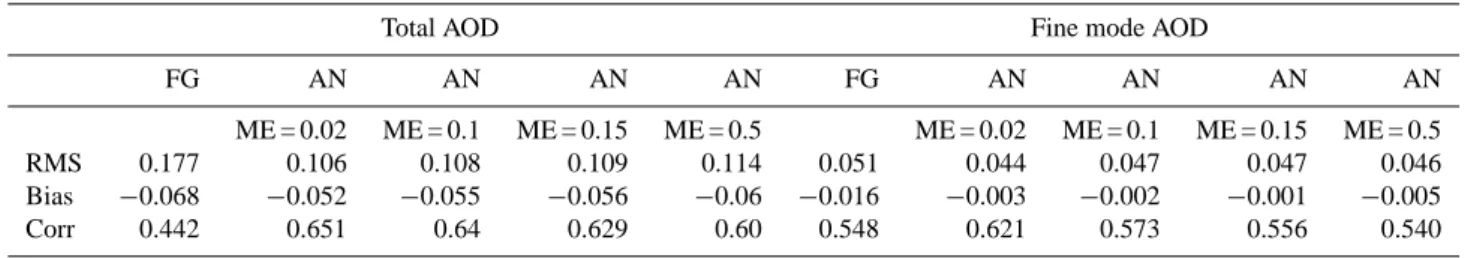
We analyze the impact on the assimilation of the uncertain-ties associated to the model errors before studying the uncer-tainties of the estimated aerosol fluxes. To analyze the impact of the model error on the results we conducted two exper-iments only differing by the magnitude of the model error. We define the model error to be equivalent to the observa-tion error over land (i.e. model error equal to 0.1 in AOD) in the first experiment and increase it further to 0.15 in the second experiment instead of 0.02 in our initial setup (Ta-ble 6). The performance of the assimilation decreases as the model error increases reflected by larger RMS errors and bi-ases and smaller correlation coefficients with respect to the initial setup. Yet both experiments perform better than the

(16)

N. Huneeus et al.: Estimating aerosol emissions by assimilating observed aerosol optical depth

Figure 8.

4599

Figure 9.

Figure 10.

Fig. 9. Annual emissions of coarse mode, fine mode and total desert dust in North West America (NWAm), South America (SAm), West Sahara (WSa), Saudi Arabia (SauAr), Africa Sub Sahara (SubSa), Australia (Au), East Asia (EAs), North East America (NEAm), India (Ind), West Asia (WAs) and East Sahara (ESa). Emission fluxes of the first guess (FG, red) and analysis (AN, black) are illustrated. Vertical bars correspond to the uncertainties in the emissions and represent one standard deviation. Regions correspond to the ones illustrated in Fig. 1.

Figure 8.

Figure 9.

Figure 10.

Fig. 10. Same as Fig. 9 but for black carbon, organic matter and sulphur dioxide for North America (NAm), South America (SAm), Europe (EU), North Africa (NAf), South Africa (SAf), Asia (As) and Australia (Aus). Emission fluxes of the first guess (FG, red) and analysis (AN, black) are illustrated as well as the emission fluxes presented in Lamarque et al. (2010) and referred as L10. To ease the comparison we have converted organic carbon (OC) emissions given in Lamarque et al. (2010) to POM as used in this study. We use a conversion factor of 1.4 between both species and therefore consider the POM flux in L10 to represent a lower boundary.

first guess in all statistics and for both total and fine mode AOD; they present smaller RMS and bias and larger correla-tion coefficient than the first guess (Table 6). Even when the model error is increased to 0.5 in AOD in a third experiment, the analysis continues to present smaller RMS errors and bias than the first guess for both total and fine mode AOD. In terms of correlation coefficient, only the fine mode presents a decrease compared to the first guess (Table 6).

The analysis error covariance matrix (A) can be computed as follows:

A = (HTR−1H + B−1)−1 (4) The elements of this matrix correspond to the errors of the estimated variable or analysis and can be used to assess the impact of the assimilation on the errors of the estimated emis-sion fluxes. The analysis errors combine the observation and model errors in R, weighted by the sensitivities of the AOD to the emissions, with the a priori errors B. The a priori an-nual emission errors (standard deviation σ ) for each region used to define the B matrix (Sect. 2.5) are 30 % for SO2,

100 % for BC and POM, 300 % for DD and 200 % for SS.

The annual errors (σ ) of the estimated emissions are 30 % for SO2, 90 % for BC and POM, 200 % for DD and 10 % for

SS. Therefore the assimilation of total and fine mode AOD reduces the errors for all species and all regions throughout the year except for SO2where the reduction is marginal.

The assimilation reduces the errors for all species and all regions throughout the year with the largest reductions for both fine and coarse DD and SS (Fig. 11a). The SS and SO2estimated fluxes present almost constant errors

through-out the year and regions (Fig. 11b). The errors associated to BB emissions present larger values in South America and Africa, especially in periods of maximum emissions from June to December, while the ones corresponding to FF emis-sions present smaller magnitudes over Europe and Asia. Fine mode DD emissions present smaller errors over the Sahara and Saudi Arabia throughout most of the year, whereas rors over Asia and the Indian subcontinent present larger er-rors mainly from March to October. Finally, for coarse mode DD the errors over Asia present larger errors from April to October, the ones of Indian subcontinent present larger errors from May to August and those over West Sahara from

(17)

Figure 11.

Fig. 11. (a) Difference in monthly mean errors (Analysis – First Guess) with the model error defined as 0.02. The monthly mean analysis error [%] for the estimated emission fluxes when the model error is defined as (b) 0.02, (c) 0.1 and (d) 0.15. The number of rows in the figure corresponds to the number of elements in the control vector. Each row corresponds to the seasonal cycle of analysis error of a given emission flux and region. The rows between different species are separated by black discontinuous lines. The red/blue colors in (a) indicate positive/negative differences whereas in (b), (c) and (d) they indicate relatively high/low values.

Table 6. Same as Table 2 but for assimilations with varying model error (ME).

FG AN AN AN AN FG AN AN AN AN

ME = 0.02 ME = 0.1 ME = 0.15 ME = 0.5 ME = 0.02 ME = 0.1 ME = 0.15 ME = 0.5

RMS 0.177 0.106 0.108 0.109 0.114 0.051 0.044 0.047 0.047 0.046

Bias −0.068 −0.052 −0.055 −0.056 −0.06 −0.016 −0.003 −0.002 −0.001 −0.005

Corr 0.442 0.651 0.64 0.629 0.60 0.548 0.621 0.573 0.556 0.540

April to August. The larger model errors usually increase the magnitude of the uncertainties for all species and all regions (Fig. 11c to d). In addition, these uncertainties are homoge-nized for each species among the regions and the differences in uncertainty between anthropogenic and dust aerosols is also increased.

4 Discussion

An inversion method has been developed that estimates the emissions of the main aerosol species and one gaseous

pre-cursor (namely DD, SS, BC, POM and SO2) by assimilating

daily total and fine mode MODIS AOD at 550 nm into an aerosol model with intermediate complexity. In spite of the additional constraint from the assimilated fine mode AOD over ocean, the total AOD presents a larger improvement over land than over ocean (with respect to MODIS) in terms of RMS error and R. This is due to the larger departures of the simulated AOD to the observed one over land than over ocean. Consistent with the above, when compared to AERONET, the total AOD also performs better over land than over ocean. However, contrary to the total AOD, a larger

(18)

improvement in RMS errors and R is seen over ocean than over land for the fine mode AOD. The contribution of assim-ilating fine mode AOD over ocean and not over land might explain this performance and reveals the prospect of imple-menting the assimilation with fine mode AOD over land.

The inspection of individual AERONET stations reveals an important mismatch between MODIS and AERONET AOD, especially at oceanic stations and those dominated by anthropogenic emissions. In addition, the comparison of statistics with respect to AERONET and the equivalent MODIS AOD suggests a representation error of continen-tal AERONET stations to capture the impact of assimilat-ing total and fine mode MODIS AOD. This mismatch and representation error could be the result of our thinning of the MODIS data necessary for their use in the assimila-tion; the loss of resolution introduces errors in the MODIS value corresponding to each AERONET station. However, a systematic bias in the MODIS fine mode AOD relative to AERONET values cannot be excluded.

The analysis error includes a coarse estimation of the model error through the R matrix. This estimation consid-ers the error introduced through grouping different aerosol species into a few tracers, a simplified chemistry, neglecting the aging of aerosols and the corresponding modification of their physical and chemical properties. A more accurate rep-resentation of the model error is a topic for a future effort, however experiments conducted varying this model error re-veal that the assimilation continues to improve the perfor-mance (in terms of RMS errors and bias) to reproduce total and fine mode AOD with model errors of 0.5 or less in AOD. The absence of a reference emission data set prevents us from validating the estimated emission fluxes directly and concluding on the final value of our results. Instead, the FG and AN emissions were compared to existing esti-mates and emission inventories. The new annual total desert dust emission of 1383 Tg yr−1 is within the range of emis-sions used in global models (Textor et al., 2006; Huneeus et al., 2011) and within the range of emissions given in Zender et al. (2004) and Cakmur et al. (2006). The former authors give an emission range of 1000 and 2150 Tg yr−1 whereas the latter estimate the emissions to be between 1500 and 2600 Tg yr−1, although emissions between 1000 and 3000 Tg yr−1 are presented as a plausible estimates. In addition, the emissions for North Africa (879 Tg yr−1) and the Middle East (39 Tg yr−1) are within the range of emis-sion given in Huneeus et al. (2011) for these regions (400– 2200 Tg yr−1 _{and 26–526 Tg yr}−1_{, respectively). The}

Mid-dle East emissions are also within the range of emissions (23–132 Tg yr−1) presented in Cakmur et al. (2006) whereas the emissions in Northern Africa are lower than the plausible emissions (964–1803 Tg yr−1) for that region given in Cak-mur et al. (2006).

The first guess (FG) and estimated (AN) emissions of BC, POM and SO2have been compared to a newer and updated

emission inventory presented in Lamarque et al. (2010),

here-after referred as L10 (Table 5). This new inventory corre-sponds to an update of previous inventories and was cre-ated to provide consistent and gridded emissions of reactive gases and aerosol for use in chemistry model simulations and to support the Intergovernmental Panel on Climate Change (IPCC) Fifth Assessment Report (AR5) (Lamarque et al., 2010). We note that the aerosol emissions in L10 actually un-derestimate the AOD peak values when used in a Chemical Transport Model (Lamarque et al., 2010) and might there-fore underestimate the real emissions. The FG emissions are larger than the L10 emissions throughout most regions ex-cept over Europe for SO2 and over Asia for BC, POM and

SO2. The larger FG emissions are consistent with a possible

underestimation of the L10 emissions mentioned above. It has also been suggested that emissions inventories may un-derestimate anthropogenic BC and POM emissions in Africa because they neglect some categories of sources and fuels (Liousse et al., 2010). In general the AN presents even larger emissions compared to L10 than the FG. Larger increase of emissions is seen for BC and POM than for SO2. The AN

emissions for these three species are reduced over Europe with respect to the FG. This is consistent with the fact that we are using somewhat outdated emission inventories and emissions are known to have decreased in Europe because of air quality policies. The biomass burning emissions have a large inter-annual variability (Granier et al., 2011) and have been increasing from the 1960s to the 1990s, at a global scale but especially over Africa and South America (Schultz et al., 2008). Therefore the increase of AN emissions of BC and POM over South America and Africa is consistent with the fact that we use as FG an estimate corresponding to periods with smaller biomass burning emissions than at present. The emissions in L10 are not within the uncertainty (σ ) of the estimated fluxes, with the exception of the emissions of BC and POM in Europe and Asia and the SO2emissions in North

and South Africa.

The general validity of the resulting emission fluxes strongly depends on the simplifications introduced in the aerosol model. Differences in processes such as sulphur chemistry and aerosol deposition as well as the definition of optical properties can influence the simulated AOD for the same emission flux. Therefore, in order to explore the general validity of the emission intensities obtained with an aerosol model with intermediate complexity, these fluxes need to be used in models with higher complexity and their simulated AOD be compared to the assimilated observations as well as independent datasets. The posterior validation of the simu-lated AOD could reveal weaknesses in the simplification that need improvement.