HAL Id: halshs-00308746
https://halshs.archives-ouvertes.fr/halshs-00308746
Submitted on 1 Aug 2008
HAL is a multi-disciplinary open access
archive for the deposit and dissemination of sci-entific research documents, whether they are pub-lished or not. The documents may come from teaching and research institutions in France or abroad, or from public or private research centers.
L’archive ouverte pluridisciplinaire HAL, est destinée au dépôt et à la diffusion de documents scientifiques de niveau recherche, publiés ou non, émanant des établissements d’enseignement et de recherche français ou étrangers, des laboratoires publics ou privés.
Brain drain, R&D-cost differentials and the innovation
gap
Fabio Mariani
To cite this version:
Fabio Mariani. Brain drain, R&D-cost differentials and the innovation gap. Recherches Economiques de Louvain - Louvain economic review, De Boeck Université, 2008, 74 (3), pp.251-272. �halshs-00308746�
Brain drain, R&D-cost differentials
and the innovation gap
∗
Fabio Mariani
UNIVERSITÉPARIS1 PANTHÉON-SORBONNE†
January 31, 2007
Abstract
This paper aims at explaining why countries with comparable levels of education still experience notable differences in terms of R&D and innovation. High-skilled mi-gration, ultimately linked to differences in R&D costs, might be responsible for the persistence of such a gap. In fact, in a model where human capital accumulation and innovation are strategic complements, we show that allowing labor outflows may strengthen educational incentives in the lagging economy if migration is probabilistic in nature, but at the same time reduces the share of innovative production. Income (growth) might be consequently affected, and a positive migration chance is very un-likely to act as a substitute for educational subsidies.
JEL classification: F22; O3; I2; J24.
Keywords: Innovation; Education; Brain drain.
1
Introduction
Some recent literature on the effects of skilled migration tends to present the brain drain as an opportunity for sending countries. In fact, papers such as Mountford (1997), Beine et al. (2001) and Stark and Wang (2002) argue that a well managed migration rate, making available higher wages (abroad) for the most skilled, can create an incentive to invest more in education, thus producing an increase in the average (after migration) domestic level of
human capital. As a consequence, skilled emigration may turn out to have beneficial
conse-quences for welfare and growth in the home economy. In particular, Stark and Wang (2002) highlight the possible role of a positive migration chance as a substitute for educational ∗I want to thank David de la Croix for his guidance and for many useful comments on earlier drafts. I am also grateful to Antonio Minniti and Luca Panaccione for insightful discussions. Finally, several comments and suggestions provided by two anonymous referees proved extremely useful to improve the paper. All remain-ing errors are, of course, under my own responsibility. Financial support from the Belgian French-Speakremain-ing Community in the framework of the ARC Project ”New Macroeconomic Perspectives on Development” (Grant ARC 03/08-302) is very gratefully acknowledged.
†CES - Centre d’Economie de la Sorbonne; 106-112, bd. de l’Hôpital, F-75013 Paris (France). Ph.: +33 (0)1 44078350; fax: +33 (0)1 44078231. E-mail: [email protected].
subsidies in less advanced countries, in order to reach the socially optimal level of human capital.
This argument may admittedly fit quite well the case of developing countries (whose growth is not led by innovative production), and then the so-called South-North brain drain. However, it proves less satisfactory with reference to the North-North high-skilled migration, since it neglects the central role played by innovation in developed economies, and by the interaction between firms’ and workers’ decisions (investments in skills and new technologies, respectively). In fact, policy makers in industrialized countries do not care only about human capital per se: they are rather concerned with the possibility to translate it into effective R&D and innovation.
Consider, for instance, the case of Europe.
One of the main concerns of European authorities in the last decade has been to fill the innovation gap with the U.S.; yet, up till now, the approach to implementing the so-called Lisbon strategy has had very limited success, and the goal of making the Union ”the most competitive and dynamic knowledge-based economy in the world” by 2010, seems completely out of sight. In fact, the European Innovation Scoreboard (European Commission, 2003) reports how Europe is still lagging behind U.S. with respect to 10 (out of 11) innovation indicators, the widest gap concerning high-tech patents. Two years later the same publication (European Commission, 2005) says that ” ... the innovation gap between the EU25 and the US is close to stable”, while ” ... the innovation gap between the EU25 and Japan is increasing”1.
The notable exception to this large and persistent gap between Europe and the U.S. is represented by the number of S&E graduates. However, as a matter of facts, many of these skilled professionals, especially top-class researchers, are crossing the Atlantic Ocean. As pointed out by the Time magazine (2004) in a recent issue devoted to Europe’s brain drain2:
”... one of the most worrying signs of their (European leaders’) failure is the continued drain of Europe’s best and brightest scientific brains, who finish their degrees and pursue careers in the U.S. [...] No wonder the U.S. has 78% more high-tech patents per capita than Europe, which is especially weak in the IT and biotech sectors.”.
If we look at country data on innovation in historical perspective, we see that, inside the OECD, some countries (Japan, Australia, Canada, Scandinavian countries, Germany, Switzerland) are converging to the U.S. innovation potential, along the last decades, while others (especially big European countries like United Kingdom, France, Italy and Spain) definitely are not (see for instance Furman et al., 2002). As far as education is concerned, we realize that, on the contrary, all European and OECD countries are progressively reach-1To give another example, Mulkay and al. (2000) analyze comparable samples of firms in France and in the U.S., to find that along the period 1979-1993, only 44% of French firms were carrying on R&D activity, while the percentage in the U.S. reached nearly 70%.
ing levels of schooling comparable to the U.S. (see Barro and Lee’s data (2000) for some compelling evidence).
Since education and R&D are usually considered to be intimately related, one could ask why only a limited group of countries has succeeded in translating higher education into stronger innovation activity. Integrating skilled migration in the analysis, we could suggest an answer to this question: although many other factors may lay behind those stylized facts, R&D-convergence might have been hampered by the consistent human capital flight mentioned above3. In fact, Docquier and Marfouk’s (2006) data on international migration
by skill support our guess: defining the ”net brain gain” (in %) as the difference between immigrants and expatriates with tertiary education or more as a proportion of working age residents, we see that most innovative countries are characterized by positive values for this variable, while lagging countries are not. To give some examples, in 2000 we have the following data: Australia + 11.4%, Canada +10.7%, Switzerland +3.8%, Sweden +2.3%, Germany +0.2%, Japan +0.1%. The main ”lagging” European countries, like UK, Italy and Spain, have negative values4, while the US (the technological leader) displays a 5.4% gain,
which corresponds, in absolute terms, to a net gain of 9,922,955 skilled workers.
Another element deserves some consideration. Kahn and Sokoloff (2004) underline how research and patenting costs were much lower in the New Continent at the dawn of technological revolution, and this was partly due to the ”institutional” costs attached to European patenting. One or two centuries after, the situation has not changed too much. In fact, as reported by the European Commission (2003), costs and fees payable for ob-taining patents in the E.U. are five times higher than in the U.S., with around 25 per cent accounted for by translation costs (European patents need to be translated into 10 different languages!). This huge difference in patenting cost, and more generally in R&D costs, could be one of the main determinants of the innovation gap between U.S. and Europe; the much better health of the R&D sector in the U.S. would explain by the same token the wage dif-ferentials that induce high-skilled researchers and IT specialists to cross the Atlantic Ocean. The goal of this paper is to translate this discussion into an analytical model: we want to study how the strategic complementarity between innovation and education is affected by migration, which is in turn related to differences in innovation costs. To accomplish this task, we will rely on a simple two-period model in the fashion of Redding (1996), charac-terized by strategic complementarities between human capital accumulation (by workers) and R&D with consequent introduction of new technologies (by a continuum of firms, that differ only by the size of their research costs). With skill-biased innovation, workers edu-cate more if they believe that a large fraction of firms is going to innovate; on the other side, 3Our explanation can be better understood if the definition of ”brain drain” is taken in its narrow sense, i.e. as the migration of extremely skilled people like scientists, engineers and top professional susceptible to be employed in R&D and innovation intensive activities.
more firms will find it profitable to innovate if workers are expected to be better educated. Differently from other models, where either all firms or none innovate, our setup would allow for an equilibrium in which only a fraction of entrepreneurs engage in R&D and then innovate. Moreover, our analysis will be based on a two-country model, thus encompass-ing the migration issue. In such a context, the brain drain affects not only human capital (as in the largest part of the existing literature about South-North brain drain), but also in-novation. In fact, a positive chance to migrate toward a more innovative country pushes the workforce to be better educated, but on the other hand outmigration reduces the num-ber of available skilled workers, discouraging innovation and R&D by domestic firms (or sectors). Assigning such a paramount role to R&D and innovation, our model looks more appropriate to fit the case of North-North skilled migration.
Our analysis is also somewhat related to a paper by Cozzi (2003)5, who addresses a
similar question about the international division of innovative labor, starting from the ob-servation that ”...the US and continental Europe have similar potentialities for R&D and comparably efficient education systems. Yet the US are active in a larger number of tech-nological sector, ... have a larger percentage of educated workers ..., and innovate rela-tively more in the aggregate.” However, there the framework of analysis was standard Schumpeterian theory, international migration played no role, and the explanation for the observed facts was that economic actors in the US have coordinated on a ”social norm” more oriented toward the defense of the national interest than in Europe (this mechanism is labeled as ”international discrimination”).
Our paper is organized as follows. After this Introduction, Section 2 presents the basic setup focusing on the domestic economy in isolation. Section 3 extends the model to con-sider a foreign country, allows for random (skilled) migration between the two economies and analyzes its consequences for the equilibrium outcome. In Section 4 the probabilistic feature is removed and migration is assumed to be endogenous in size: the whole model is solved again to account for these changes. Finally, a concluding discussion is provided in Section 5.
2
The basic model (autarky)
We will start by the description of the home economy as being in isolation, i.e. as if frontiers were closed: international labor mobility is not allowed.
The home economy is populated by continua of non-overlapping, two-period lived workers and entrepreneurs; the latter might be identified with firms or even with pro-ductive sectors. In absence of migration, there would be l workers for every firm. Both
workers and entrepreneurs maximize the following utility function:
U(x1, x2) =x1+σx2, (1)
where xtdenotes consumption at time t and σ (<1) accounts for intertemporal preferences.
Since savings are excluded from our analysis, utility maximization coincides with the max-imization of lifetime income (respectively wages and profits).
2.1 Firms (entrepreneurs)
In every period (t=1, 2) each firm produces its output according to:
Yt= Atltht, (2)
where htdefines the human capital of the representative worker and Ata productivity
pa-rameter, while ltis the number of workers employed by the firm and it will be normalized
to 1 throughout the rest of the paper.
Output is split between profits and wages according to distributive quotas π and(1− π), that we assume to depend on institutional settings and to stay constant in the two periods (exactly as in Redding, 1996).
The productivity parameter Atmay change over time as a result of investments in R&D
and innovation. In fact, a representative firm i can shift its productivity from A1 = 1 to
A2 = λ > 1, if its manager bears a research cost equal to αi in period 16. The size of this
innovation cost is the only source of heterogeneity among firms. For sake of simplicity, we assume αi to be uniformly distributed over the interval [0, c]. We will show that, as a
consequence of this cost distribution, only a fraction p of firms (or sectors) will choose to engage in R&D and achieve innovation7.
2.2 Workers
Workers are born homogeneous: all of them are naturally endowed with human capital
h. Let us underline that, although we have only one category of workers, we conceptually
refer to skilled workers8(researchers, for instance).
In the first period they devote a fraction v or their time to formal schooling; in the remainder of the period (1−v) they work, after having been randomly matched with the
different firms. They contribute to production according to h1 = (1−v)h.
In period 2 they reach a human capital level equal to h2 = f(v, h), with f(v, h)being
the production function of human capital through education. We assume that, after the 6By assumption, this cost does not concern workers: it affects only profits.
7We could also have assumed, somewhat more realistically, that actual innovation occurs with a probability ζ∈ (0, 1)if the R&D effort is made. However, our analysis would not have produced different results.
8Adding a class of unskilled workers would not change the substance of the paper, provided that social mobility is not allowed.
random matching occurred in the first period, workers are tied to firms by a contract whose duration spans over their whole lifetime. By consequence, each worker has a probability p to be matched, in the second period, with a firm that has done R&D and, having innovated, is more productive9.
The hypothesis of lifetime contracts characterizes Redding’s (1996) and Acemoglu’s (1994) models as well. We propose to interpret this assumption as a consequence of pro-hibitively high mobility costs between firms; if we take firms as different production sec-tors, this looks quite realistic, meaning that a skilled worker or a researcher who has been employed in the chemical sector during period 1 is not likely to maintain her productivity if she is hired by a software industry in period 2 (in other words we are assuming that work-ers build ”firm-specific” abilities in the first period)10. By consequence, mobility between
different sectors in the same country is more costly than international mobility between firms acting in the same sector, and we are eventually allowed to deal with international migration (Sections 3 and 4).
2.3 Optimal choices
The representative worker chooses v to maximize her expected lifetime labor income:
E(ω) = (1−π){(1−v)h+σ[pλ+ (1−p)]f(v, h)}. (3) This formulation takes into account that workers have a probability p to be matched with a more productive firm, thus being paid a higher unit wage in the second part of their working life. It is also clear that the production function for human capital plays a crucial role. We choose to adopt a formulation of the type: f(v, h) =h(1+g(v)), and in particular:
f(v, h) =h(1+γ√v). (4) This square root specification proves particularly useful to get closed-form solutions. However, the more general form f(v, h) = h(1+γvθ)would generate the same results, in
qualitative terms, for a wide range of values of the parameter θ11.
Solving∂E(ω)/∂v=0 leads to:
vw = 0 if vw(p) ≤0 vw(p) if 0<vw(p) <1 1 if vw(p) ≥1 , (5)
9Otherwise, if workers and firms were free to renegotiate contracts after period 1 (once R&D decisions are eventually revealed), the most efficient firm would hire the whole workforce, since the production function is linear in ht. With decreasing returns to labor, the best firm would also be the largest, and less innovative
firms would hire less people; this outcome would sound more realistic, but it would come at the expense of the analytical tractability of the rest of the model.
10The degree of realism of this assumption depends positively on the skill level and the degree of specializa-tion of workers.
where:
vw(p) = 14σ2γ2[1+p(λ−1)]2. (6)
Optimal education depends positively on p (strategic complementarity); not surpris-ingly it also increases with the size of innovation (λ), with the productivity of time in edu-cation (γ), and with the preference for the future (σ).
On the firms’ side, an entrepreneur will choose to bear the R&D cost if and only if the following inequality holds:
π(Y1−αi+σY2I) >π(Y1+σY2), (7)
i.e. if the second period output with innovation (YI
2) will be high enough to cover research
costs. Of course, there is a threshold value for α (call it bα) which makes an entrepreneur in-different between innovating and staying put with the ”old” technology. This value solves: (1−v)h−α+σ λ(1+γ√v)h = (1−v)h+σ(1+γ√v)h, (8)
and it is then equal to bα= (λ−1)σ(1+γ√v)h.
Therefore, every firm characterized by αi <αbwill choose to innovate. Assuming h=1,
and recalling that αiis uniformly distributed over the interval[0, c], the fraction of
innovat-ing firms is given by:
pf = 0 if pf(v) ≤0 pf(v) if 0< pf(v) <1 1 if pf(v) ≥1 , (9) where: pf(v) = (λ−1)σ(1+γ√v) c . (10)
Innovation is then a strategic complement to the educational choice made by workers (v); it is also a positive function of λ, σ and γ.
2.4 Equilibrium
We look for a rational expectation equilibrium: workers’ and entrepreneurs’ decisions are mutually dependent. Moreover, as we have seen, investment in R&D and investment in education can be defined as strategic complements.
We define a rational expectations (Nash) equilibrium as a pair(pǫ, vǫ), such that
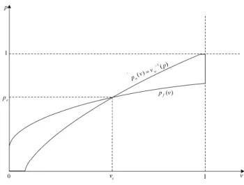
work-ers’ expectations upon firms’ choice are realized, and vice versa. All the eventual inter-sections between the two curves pf and vw in the (p, v)space are equilibria of this type;
potentially we may even have multiple equilibria, but we restrict our attention to those equilibria that are characterized by 0 < pǫ < 1 and 0< vǫ < 1, thus excluding situations
The interior equilibrium is completely described by the values of the educational choice
vǫand the share of innovative firms pǫ, that can be found solving the following system of
two equations in two unknowns: ( pf(v) = (λ−1)σ(1+γ √ v) c vw(p) = 14σ2γ2[1+p(λ−1)]2 . (11)
The solution pair is consequently given by: pǫ= (2+σγ 2)σ(λ−1) 2c−σ2γ2(λ−1)2 vǫ= σ 2γ2[c+(λ−1)2σ]2 [σ2γ2(λ−1)2−2c]2 . (12)
2.5 Characterization of the equilibrium
To ensure the existence of an interior equilibrium described by (12), we need to define con-ditions on the parameters, such that both pǫand vǫbelong to the (0, 1)interval. To have
0< pǫ <1 we need c>σ(λ−1)(2+σγ2λ)/2. On the other hand, 0< vǫ <1 holds when
either c <γ(γ−1)(λ−1)2σ2/(2+σγ)or c>γ(γ+1)(λ−1)2σ2/(2−σγ). Summing up, an interior equilibrium does exist if:
c>max· 1 2σ(λ−1)(2+σγ2λ); γ(γ+1)(λ−1)2σ2 2−σγ ¸ .
To ensure the stability of the interior equilibrium, we need the ”reaction function” of workers (pw(v), which is the inverse function of equation (6)) to be steeper than the one of
firms (equation (10)). A sufficient condition for this to be case is simply c>σ2(λ−1)2γ2/2 (c is a crucial parameter since it determines the slope of the firms’ best-reply function). It is then easy to check that the existence of an interior equilibrium implies its stability.
Figure 1 reproduces the case where an interior (and stable) equilibrium exists. Two other possible equilibria ((0, 0)and(1, 1)) arise as corner solutions; however, both of them are unstable.
3
The two-country model with probabilistic migration
Until now we have considered the economy as being in isolation. How does the picture change if we assume that there also exists a foreign economy offering higher wages, to which home workers may eventually want to migrate?
Let us underline that in this Section we treat migration as an endogenous choice (we will describe a situation that generates higher expected wages on the foreign labor market, and then makes a potential migrant of every home worker), but exogenous in its size: in fact, we assume that only a fraction m of the domestic workforce is actually allowed to go
Figure 1: A stable interior equilibrium exists
abroad. Therefore, as in most of the brain drain literature12, migrants are assumed to be
randomly selected; the case of self-selection will be analyzed in Section 4.
Moreover, we assume that high-skilled workers are internationally mobile, while en-trepreneurs (firms) are not. This assumption deserves some explanation, since it may seem to be at odds with the usual hypothesis of capital being more mobile than labor. Our choice is driven by a couple of considerations. First, the kind of labor we are dealing with here is indeed quite special: engineers, scientists and top researchers are in fact highly mobile and their competences are not very country-specific (for instance, they are supposed not to undergo any skill depreciation due to a poor knowledge of the host country’s language). Second, even if the international mobility of capital is progressively increasing, it is also true that the international relocation of firms (or entire productive sectors) is something differ-ent13: it would take more time than the migration of a skilled worker and imply fixed costs
that are not negligible. As remarked by Janeba (1998), the strategic trade theory literature usually assumes international immobility of firms (producing in the country of residence of their owners), while the tax competition literature considers that firms are mobile and exploit tax differential through their location choice. We prefer to stick to the first type of assumption, and propose to assume that firms are mobile only in the long run14.
Finally, we assume that also with labor mobility all firms will have the same number of workers, so that, due to migration, every entrepreneur will lose a fraction m of her work-force.
12See for instance Mountford (1997) and Beine et al. (2001).
13A given entrepreneur may continue to run a firm in her country even if some capital is flowing away (or if some of her employees are leaving).
14Even in a paper on capital tax competition, Wilson and Wildasin (2004) admit that physical capital is only
3.1 Innovation in the foreign economy
We model the foreign economy as being absolutely identical to the home economy, with only one but crucial exception, which concerns the size of innovation costs.
In fact, we assume that a foreign entrepreneur who wants to undertake R&D in order to produce innovation and enhance the productivity of her firm, has to bear a fixed cost αi∗ = αi−d. The parameter d accounts for some kind of technological, organizational, or
”institutional” factor that makes R&D more costly in the home economy, as suggested by Kahn and Sokoloff (2004). As a consequence, the fraction of innovative firms in the foreign country is given by p∗ =min[p+η; 1], where η=d/c15. In the remainder of the paper we
will implicitly assume η < 1−p, to avoid analytical complications; as a consequence we
will always work with p∗= p+η6=1.
It is important to say that p∗ can be taken as exogenous (with respect to immigration)
as long as the sending country is considered to be small. This ”small-country” hypothesis keeps the model analytically tractable, without entraining any loss of generality. In fact, it is true that sizable skilled immigration, increasing the number of workers per firm in the foreign country, would also affect the joint determination of innovation and schooling in the foreign economy. But, since we take the perspective of the sending country, it seems reasonable to assume that skilled migration from this single country represents a negligible contribution to the foreign labor market. However, the sum of all the migration inflows coming from different countries is not negligible from the point of view of the receiving country: Subsection 3.5 is devoted to the analysis of this aspect.
Let us also underline that in our setting expected wage differentials are ultimately mo-tivated by international differences in R&D costs. Many additional explanations for wage gaps are plausible and important: for instance we might have assumed that innovation is larger in size or more productive abroad (λ∗ > λ) to explain a higher expected wage;
however, we think that this is not a crucial point for our analysis, whose generality is not affected by the simplicity of our assumptions.
3.2 Consequences for the home economy
3.2.1 Timing of events
As in autarky, skilled workers are matched with entrepreneurs (firms/sectors) in the first period. This matching process takes place randomly, since firms have not yet revealed their cost structure and workers are identical. The matching is then sealed by lifetime contracts, thus ruling out inter-sectoral mobility. We identify a positive migration chance as the possibility, for a fraction m of workers, to break their contract and work with a foreign
15Alternatively, we could have assumed α∗
i =αi, but c∗=δc, with 0<δ<1. As a consequence we would
have had p∗=pχ, where χ=1/δ. This ”multiplicative” specification would determine qualitatively the same results that we obtain employing the ”additive” specification.
firm operating in the same sector16. The random draw of these m workers is supposed to
take place before the R&D outcome of domestic firms is revealed17. 3.2.2 Workers
The representative worker knows that if she goes on the foreign labor market in the second period, her expected lifetime wage will be:
E(ω∗) = (1−π){(1−v)h+σ[p∗λ+ (1−p∗)]h(1+γ√v)} >E(ω). (13) Since migration is possible (with probability m), in this new framework she will select
vin order to maximize E(ωM) = mE(ω∗) + (1−m)E(ω). From∂E(ωM)/∂v = 0, we get
the optimal choice for v, when migration is allowed:
vw,M = 0 if vw,M(p) ≤0 vw,M(p) if 0< vw,M(p) <1 1 if vw,M(p) ≥1 , (14) where: vw,M(p) = 14σ2γ2[1+ (p+mη)(λ−1)]2. (15)
Comparing (15) with (6) we see that migration can exert an inducement effect on the schooling choice of home workers. In fact, migration can be regarded as a possibility that enhances the option value of education (as shown by the inequality in (13)), thus fostering education investment.
Therefore, as long as firms’ strategies are not considered, migration may be seen as an opportunity from the viewpoint of the representative worker18.
3.2.3 Firms
The prospective human capital flight alters the strategy of the entrepreneurs: every firm is going to lose a fraction m of its workforce, and this fact will entrain, ceteris paribus, a reduction of its output in the second period. The arbitrage condition for the entrepreneur then becomes:
(1−v)h−α+σ λ(1−m)(1+γ√v)h = (1−v)h+σ(1−m)(1+γ√v)h, (16)
and the indifference value for α is now equal to bαM = (1−m)(λ−1)σ(1+γ√v)h. As a
consequence, in this environment with labor mobility, the fraction of innovating firms is 16This way to introduce migration captures quite well the fact that highly specialized European workers may prefer to go on the American labor market to take more profit from their field of specialization.
17This assumption implies that even the most innovative firms will suffer from a loss of skilled employees and consequently generates a negative effect of ”aggregate” uncertainty on the whole production system.
18With p fixed, even those who don’t migrate do not experience a decrease in their income; moreover, if human capital does not enter linearly the production function, they have their wages increased.
given by: pf,M= 0 if pf,M(v) ≤0 pf,M(v) if 0< pf,M(v) <1 1 if pf,M(v) ≥1 , (17) where: pf,M(v) = (1−m)(λ−1)σ(1+γ √ v) c . (18)
It can be noticed that the function pf,M(v), differently from vw,M(p), does not depend
on η.
3.2.4 The equilibrium with migration
The ”new” equilibrium(pǫ,M, vǫ,M)can be found following the same procedure we applied
in Section 2. In fact, as a solution for: ( pf,M(v, m) = (1−m)(λ−1)σ(1+γ √ v) c vw,M(p, m) = 14σ2γ2[1+ (p+mη)(λ−1)]2 , (19) we obtain: pǫ,M = (1−m)[2+σγ 2(1+mη(λ−1))]σ(λ−1) 2c−(1−m)σ2γ2(λ−1)2 vǫ,M = σ 2γ2[c(1+mη(λ−1))+(1−m)(λ−1)2σ]2 [(1−m)σ2γ2(λ−1)2−2c]2 . . (20)
It is now quite easy to assess the effect of migration on the equilibrium values of educa-tion and innovaeduca-tion, respectively.
Proposition 1 The fraction of innovating firms decreases with the probability of migration, while the relationship between the level of education and the probability of migration is ∪-shaped. In fact, there exists a threshold value c for R&D costs such that, if c < c, the equilibrium length of schooling decreases with the migration chance as well, while, for every c >c, a growing probability of migration induces the agents to get more and more education.
(The Proof is given in Appendix A)
Taken together, these results say quite clearly that a brain drain is very unlikely to bene-fit the home economy, and explain why higher education may not imply more innovation. A country that experiences a human capital flight loses innovative potential at the same time, even if its workforce becomes more and more educated on average. This is due to the negative effect of m on R&D decisions taken by the firms.
Whether migration affects skill accumulation negatively or positively depends on R&D costs (c). The intuition for the non-monotone result given in Proposition 1 is the following: if c is low enough, it means that the equilibrium value of p in autarky is quite close to 1, and the potential gains from emigration are not very large; on the other hand, with a very high
c, p would be extremely low in autarky: as a consequence, the relative returns to migration
3.3 Can emigration policy act as a substitute for educational subsidies?
We would also underline that, in contrast with Stark and Wang (2002), our analysis would not trust emigration policy as a valuable substitute for educational subsidies. Stark and Wang neglect the adverse effects of a brain drain on firms’ strategies. In fact, although a positive migration chance does generate, from the workers’ viewpoint, an incentive to edu-cate more, it also affects negatively the optimal choices of the firms, leading to a suboptimal equilibrium outcome if strategic complementarities matter. Educational subsidies are not characterized by this kind of shortcoming, and thus they cannot be ”easily” replaced by a virtuous emigration policy19.
3.4 What about average income?
Although it is not the main purpose of the paper, it could be interesting to assess the net im-pact of migration on average income. In fact, we have seen that a positive migration chance may happen to exert effects of opposite sign on education and innovation, respectively.
We try to evaluate the average lifetime income of the home economy (once migration is actually taken into account), that is:
ψ(m) = Y1(m) −C(m)
1+l +σ
pMY2I(m) + (1−pM(m))Y2(m)
1+l(1−m) , (21)
where C(m)is the total amount of research costs. Normalizing l to 1, the expression above can be rewritten as:
ψ(m) = h(1−vM) −π RαˆM 0 α(1/c)dα 2 +σ (1−m)h(1+γvθM)[pMλ+ (1−pM)] 1+ (1−m) . (22)
This formulation of average income, neglecting the earnings of emigrants in period 2, considers domestic income instead of national income20.
Since many different variables are involved, it would be very problematic to study the sign of the function∂ψ/∂m. However, we can assume that θ = 1/2, σ =1 and h = 1, and concentrate on limm→0∂ψ(m)/∂m, to assess the marginal effect of opening the frontiers on
income.
We find that limm→0∂ψ(m)/∂mis a monotonically increasing function of η; in particular
it is positive for:
η> ˆη= 2c
2+c[6+γ2+2π(2+γ2)](λ−1)2−γ2(λ−1)4
(1+π)γ2[2c−γ2(λ−1)2](λ−1)3 .
19Though in a different framework, Stark and Wang’s hypothesis of substitutability between migration and subsidies is also challenged by Docquier et al. (2005).
20Since emigration is random and the identity of future emigrants is unknown a priori, it is not clear whether (22) might be also interpreted as a social welfare function.
Admissible values for η go from 0 to ¯η = 1−pM; then, if ¯η < ˆη it will be possible to
conclude that∂ψ/∂mis negative for m→0. Now, ˆη− ¯η, writes as:
−1+ c (1+π)γ2(λ−1)3 + 3+γ2+π(2+γ2) (1+π)γ2(λ−1) + 2(2+γ2)(λ−1) 2c−γ2(λ−1)2 ,
and it can become negative only if c is very low. But c cannot be lower than cℓ = (1/2)(λ−
1)(2+λγ2)(value for which p would be equal to 1). It is easy to check that: lim
c→cℓ(ˆη−¯η) =
2π(λ−1)(2+λγ2) +λ[6+γ2(2λ−1)] −4 2(1+π)γ2(λ−1)2
and this limit is indeed positive for reasonable values of the parameters, let’s say for 1 < λ< 2 and 0<γ <1. By consequence a ”marginal” increase of international mobility will decrease average lifetime income in the sending country.
Migration may be more likely to be beneficial in quite extreme cases. Think for instance to an economy where, without migration, no firm would engage in innovation. Such a case is not covered by our previous analysis, that was considering only interior solutions for p and v; however, it implies that an educational gain does not entrain any loss in terms of innovation: a higher v is paid only by a positive m (loss of skilled workers), without deter-mining any decrease in p. The behavior of the firms being unaffected, this case reproduces the usual story told by Stark and Wang (2002) about a brain drain vs a brain gain, and the net effect might even be positive, for low values of m.
3.5 Consequences for the foreign economy
Without going into analytical details, we can spend some words on the effects of labor mo-bility on the destination country. Let us underline that, although the contribution of each single sending country may be assumed to be negligible (”small country” hypothesis), the sum of all migration inflows is not negligible, from the viewpoint of the receiving economy. In our setting, the arrival of a number of (highly educated) immigrants does not affect the strategy choice of foreign workers, who will not experience any decrease in wages21.
But on the other side, firms’ strategies are indeed affected: a fully anticipated arrival of skilled immigrants will make the rewards from innovation more valuable, so that the curve
p∗f(v, m)will shift up, leading to a ”new” equilibrium with both p∗
ǫand v∗ǫhigher than they
would have been in the case without labor mobility. Therefore, skilled immigration would be unambiguously beneficial for the destination country.
4
Endogenous size of migration
In this Section we propose to remove the assumption that an exogenously fixed fraction
mof workers is allowed to migrate. Instead of being randomly out-selected (by effect of
21This depends on the assumptions upon which our model is built, but it does not produce an excessively unrealistic feature, at least as far as skilled workers are concerned.
emigration quotas, for instance), workers are now assumed to be self -selected. To allow for self-selection of migrants, and in order to fully endogenize m, we introduce one fac-tor of heterogeneity among workers, namely an individual-specific effect of living abroad on personal utility. Then, we assume that every worker who wants to migrate can do it without any impediment: the migration choice will depend on the wage differential and on the utility cost of migration. As a consequence, m will be a function of the distribution of a disutility parameter and the potential wage differential. On the other side of the labor market, domestic firms don’t know m in advance.
Now, we put under scrutiny the consequences of openness for the equilibrium on the domestic labor market.
4.1 Firms
Firms act as before, but with one exception: they are not informed about the actual value of
m. The optimal strategy of every entrepreneur consists in choosing whether to innovate or not, depending on the possible values of m and v. As an aggregate, for every possible pair (v, m), firms ”select” that value of p which maximizes their expected profits. Hence, once we ignore eventual corner solutions:
pf(v, m) =
σ(1−m)(λ−1)(1+γ√v)
c . (23)
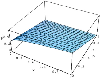
The set of firm strategies can be represented in the 3-dimension (p, v, m) space as a surface (see Figure 2). It is easy to check that∂pf(v, m)/∂v> 0 and∂pf(v, m)/∂m< 0.
0 0.2 0.4 0.6 0.8 1 v 0 0.2 0.4 0.6 0.8 1 m 0 0.2 0.4 p 0 0.2 0.4 0.6 0.8 v
Figure 2: Firms’ strategy p=p(v,m)
4.2 Workers
Home workers’ strategy consists in reacting to every possible p with the optimal choice for (m, v); of course, m is the optimal choice of the workers as an aggregate (like p for firms):
every single worker individually makes a binary choice (moving or staying). We will show that the choices of m and v are mutually tied, so that the set of workers’ strategies can be thought of as a curve in the 3-dimension(p, v, m)space.
In fact, in order to decide whether to migrate or not, workers compare the maximum lifetime incomes attainable at home and abroad, respectively. Going abroad, the total in-come of the i-th worker would be:
E(ω∗) = (1−π){(1−vM)h+σ[p∗λ+ (1−p∗)]h(1+γ√vM)} −κi, (24)
where p∗ = p+η as before, v
M is the value of education which maximizes income if
migration is selected, and κi = (1−π)µi accounts for the pecuniary expression of the
utility loss that the i-th worker would incur living abroad instead of staying in her home country. We assume µ to be uniformly distributed over the interval[0, Q].
Staying at home, total income writes as:
E(ω) = (1−π){(1−vH)h+σ[pλ+ (1−p)]h(1+γ√vH)} −ι, (25)
where vH is the income-maximizing value of education if the second period is spent on
the domestic labor market, while ι = (1−π)ξ stands for some cost linked to working at home (we may think to higher interaction costs in performing research activity, lower social consideration of intellectual jobs in the home country, lower on-the-job satisfaction22, etc.).
The i-th worker opts for migration if E(ω∗) >E(ω), i.e. if:
µi <µ =ξ− (vF−vH) + [1+ (p+η)(λ−1)]σ(1+γ√vF) − [1+p(λ−1)]σ(1+γ√vH);
(26) by consequence, the fraction of workers who choose to migrate is given by m(p) = µ/Q.
Taking the inverse function, we can write:
p(m) = 4(mQ−ξ) −ησ{4+σγ
2[2+η(λ−1)]}
2ησ2γ2(λ−1)2 . (27)
In this setting all the workers who migrate choose vM, while those who stay educate at
the level vH, so that, in contrast with the case we analyzed in Section 3, there is no incentive
effect linked to migration23. Let us also recall that:
vH(p) = 14σ2γ2[1+p(λ−1)]2. (28)
To sum up, the workers’ strategy (on the domestic labor market) is given by: pw(m) = 4(mQ−ξ)−ησ{4+σγ 2[2+η(λ−1)]} 2ησ2γ2(λ−1)2 pw(v) = 2 √ v−σγ σγ(λ−1) , (29)
which represents, as pointed out before, a curve in the(p, v, m)space.
22In fact, many European scientists who work in the U.S. often complain about difficult research conditions and the less meritocratic environment in Europe (TIME Magazine Europe, ibid).
23We could also imagine an intermediate situation, in which both heterogeneity w.r.t. foreign consumption and probabilistic success of migration are considered. Our results would go through.
4.3 Equilibrium
To determine equilibrium values, we need to find the intersection between curve (29) and surface (23), solving the system composed by (23) and (29). For sake of simplicity, we assume σ =1, γ= 1 and ξ =0, so that we can rewrite the whole system as:
p(v, m) = (1−m)(λ−c1)(1+√v) p(m) = 4mQ−η{24η+[(λ−2+η(λ−1)2 1)]} p(v) = 2√λ−v−11 , (30) or, equivalently: pf(v, m) = (1/c)(1−m)(λ−1)(1+√v) vw(p) = (1/4)[1+p(λ−1)]2 mw(p) = (1/4Q)η(λ−1)[(2p+η)(λ−1) +6] . (31)
A solution to this system of three equations in three unknowns does exist, it is unique and it is given by the triple(pE, vE, mE).
We are now interested in establishing how the home economy outcomes change if fron-tiers are open. Given that, in our setting, migration ultimately depends on international differences in R&D costs (η), we look at the effects of η on mE, pE and vE. We can claim
what follows:
Proposition 2 If labor mobility is allowed and migrants are self-selected (rather than randomly out-selected), actual migration rates increase with R&D-cost differentials; moreover, η affects negatively both innovation and education; i.e.: ∂mE/∂η>0,∂pE/∂η<0 and∂vE/∂η<0.
(The Proof is given in Appendix B)
This result prospects a worse situation, with respect to the case of probabilistic migration; this is due to the lack of any inducement effect: all the workers who still act on the home labor market have not migrated by their own choice, and then they have not benefited from any educational incentive. Therefore, if migration is despoiled of its random feature, labor mobility is not only unable to induce more innovation, but it also fails to break the low-skill/low-innovation link, since there are no human capital gains for ”sedentary” workers.
5
Conclusions
In this paper, we have tried to decompose the effect of a brain drain on economic perfor-mance into two distinct effects, respectively on human capital accumulation and innova-tion.
We have shown that, due to strategic complemetarities between education and R&D , a positive (and exogenous) migration chance might indeed favor human capital accumu-lation by workers in the less innovative country, but may not increase at the same time
the fraction of national firms that engage in R&D and innovation. This result could help explaining why many European countries are not able to close the innovation gap with the U.S., although the educational attainment of their workers is steadily increasing toward the highest standards. Seen in a more general perspective, our findings also suggest that migra-tion policies should not be trusted as possible substitutes of educamigra-tional policies, because of their adverse effects on firms’ strategies.
We have also tried to relax the assumption of probabilistic migration. If the size of mi-gration is endogenous, being entirely determined by workers’ preferences and differences in innovation costs, the consequences of the brain drain for the home economy are defi-nitely worse: since only migrants are induced to educate more, and no incentive effect acts for those workers who choose to stay home, there is no hope to use emigration policies in order to enhance economic performance.
References
[1] Acemoglu, D. (1994): ”Search in the labour market, incomplete contracts and growth”,
CEPR Discussion Paperno. 1026.
[2] Barro, R.J. and J.-W. Lee (2000): ”International data on educational attainment: updates and implications”, CID Working Paper no. 42. [Data set available at: www.cid.harvard.edu/ciddata/ciddata.html]
[3] Beine, M., F. Docquier and H. Rapoport (2001): ”Brain drain and economic growth: theory and evidence”, Journal of Development Economics 64, 275-289.
[4] Cooper, R. and A. John (1988): ”Coordinating coordination failures in Keynesian mod-els”, Quarterly Journal of Economics 103 (3), 441-463.
[5] Cozzi, G. (2003): ”The self-fulfilling international allocation of innovation, inequality, and education”, mimeo.
[6] Docquier, F. and A. Marfouk (2006): ”International migration by education attainment, 1990-2000”; in Ozden, C. and M. Schiff (eds.): International Migration, Remittances & the
Brain Drain, World Bank and Palgrave Macmillan.
[7] Docquier, F., O. Faye and P. Pestieau (2005): ”Is migration a good substitute for educa-tion subsidies?”, mimeo.
[8] European Commission (2003, 2005): European Innovation Scoreboard, Cordis, Luxem-bourg. [Available on-line at: http://trendchart.cordis.lu/]
[9] Furman, J.L., M.E. Porter and S. Stern (2002): ”The determinants of national innovative capacity”, Research Policy 31, 899-933.
[10] Janeba, E. (1998): ”Tax competition in imperfectly competitive markets”, Journal of
International Economics44, 135-153.
[11] Kahn, B.Z. and K.L. Sokoloff (2004): ”Institutions and technological innovation during early economic growth: evidence from the great inventors of the United States, 1790-1930”, mimeo.
[12] Mountford, A. (1997): ”Can a brain drain be good for growth in the source economy?”,
Journal of Development Economics53, 287-303.
[13] Mulkay, B., B.H. Hall and J. Mairesse (2000): ”Firm level investment and R&D in France and the United States: a comparison”, NBER Working Paper 8038.
[14] Redding, S. (1996): ”The low-skill, low-quality trap: strategic complementarities be-tween human capital and R&D”, Economic Journal 106 (435), 458-470.
[15] Stark, O. and Y. Wang (2002): ”Inducing human capital formation: migration as a substitute for subsidies”, Journal of Public Economics 86, 29-46.
[16] Wilson, J.D. and D.E. Wildasin (2004): ”Capital tax competition: bane or boon”, Journal
of Public Economics88, 1065-1091.
A
Proof of Proposition 1
The function∂pǫ,M/∂mwould be positive only if:
c< − ησ
3γ4(1−m)2(λ−1)3
4+2σγ2[1+ (2m−1)η(λ−1)],
which cannot never be true since the r.h.s. is always negative. Then, ∂pǫ,M/∂m must be
always negative.
Studying the sign of the function∂vǫ,M/∂m, we find that it is negative for c < c < c,
where: c= σ 2γ2 2 (1−m)(λ−1)2, and c= σ 2η{2+σγ2[1+η(λ−1)]}(λ−1).
However, we can discard all those values of c that would imply corner solutions for pǫ,
i.e. pǫ≥1 in (12). Since the latter would hold for c≤co, where:
co =
σ
2(λ−1)(2+σγ2λ),
B
Proof of Proposition 2
As a solution of system (31), we obtain: pE = −R+ √ S−η[12+η(λ−1)](λ−1)3 4η(λ−1)4 vE = {R− √ S+η[8+η(λ−1)](λ−1)3}2 64η2(λ−1)6 mE = −R+ √ S+η2(λ−1)4 8Q(λ−1)2 , (32) where: R=4Q[2c− (λ−1)2], and S=R2+8ηQ{2c[12+η(λ−1)] −η(λ−1)3}(λ−1)3+η4(λ−1)8. Then, we consider the first derivatives with respect to η, starting by:
∂mE ∂η = (λ−1)[η(λ−1) + √T S] 4Q , where: T= 8cQ[6+ (λ−1)η] +η(λ−1)3[η2(λ−1)2−4Q].
It is easy to check that∂mE/∂η is always positive (i.e. ∀η ∈ (0, 1)), provided that c >
(λ−1)2/2.
Let’s now turn to ∂pE/∂η and ∂vE/∂η: after some tedious calculations, it is possible
to show that they are both negative. However, to get a straight intuition we suggest to consider their limits for η →0, obtaining:
lim η→0 ∂pE ∂η = − 18c2(λ−1)2 Q[2c− (λ−1)2]3, and lim η→0 ∂vE ∂η = 18c2(λ−1)3[c+ (λ−1)2] Q[2c− (λ−1)2]4 .
It can be easily seen that the second expression is always negative, while the first is negative if c> (λ−1)2/2.
However, the latter is not a restriction, since values of c lower than(λ−1)2/2 would cause p+ηto be larger than 1, and must then be discarded in order to meet our assump-tions.