Matrimonial Ring Structures

(1)

HAL Id: halshs-00119444

https://halshs.archives-ouvertes.fr/halshs-00119444

Submitted on 9 Dec 2006

HAL is a multi-disciplinary open access

archive for the deposit and dissemination of sci-entific research documents, whether they are pub-lished or not. The documents may come from teaching and research institutions in France or abroad, or from public or private research centers.

L’archive ouverte pluridisciplinaire HAL, est destinée au dépôt et à la diffusion de documents scientifiques de niveau recherche, publiés ou non, émanant des établissements d’enseignement et de recherche français ou étrangers, des laboratoires publics ou privés.

Douglas White

To cite this version:

Klaus Hamberger, Michael Houseman, Isabelle Daillant, Laurent Barry, Douglas White. Matrimo-nial Ring Structures. Mathématiques et Sciences Humaines, Centre de Mathématique Sociale et de statistique, EPHE, 2004, pp.83-119. �halshs-00119444�

(2)

Math. & Sci. hum. / Mathematics and Social Science, (42e_{année, 2004(4), p. 83-120)}

MATRIMONIAL RING STRUCTURES

Klaus HAMBERGER1, Michael HOUSEMAN1, Isabelle DAILLANT1, Douglas R. WHITE2 and Laurent BARRY3

RÉSUMÉ – Les anneaux matrimoniaux : une approche formelle

Les anneaux matrimoniaux sont un type particulier de cycles qui se constituent dans les réseaux de parenté lorsque les conjoints sont liés entre eux par des liens de consanguinité et d’affinité. En adoptant une approche relevant de l’analyse des réseaux, l’article tente d’aborder la théorie structurale de la parenté sur une base générale permettant de dépasser l’examen de types singuliers d’anneaux (comme le « mariage de cousins croisés », l’« l’échange de sœurs », etc). Il offre une définition et une analyse formelle des anneaux matrimoniaux, une méthode d’énumération de toutes leurs classes d’isomorphisme au sein d’un horizon généalogique donné. Cette approche permet d’étudier les configurations d’anneaux dans des réseaux de parenté empiriques. L’article fournit aussi les moyens techniques pour mener ces analyses avec le programme informatique PAJEK. Un dossier contenant les macros nécessaires peut être téléchargé sur le web. La méthode est illustrée à l’aide de réseaux de parenté provenant de quatre continents (Amérique du Sud, Afrique, Australie et Europe.

MOTS-CLÉS – Anneaux matrimoniaux, Parenté, Analyse des réseaux sociaux, Théorie des graphes, Théorie de l’énumération, Anthropologie sociale

SUMMARY – The paper deals with matrimonial rings, a particular kind of cycles in kinship networks which result when spouses are linked to each other by ties of consanguinity or affinity. By taking a network-analytic perspective, the paper endeavours to put this classical issue of structural kinship theory on a general basis, such as to allow conclusions which go beyond isolated discussions of particular ring types (like “cross-cousin marriage”, “sister exchange”, and so forth). The paper provides a definition and formal analysis of matrimonial rings, a method of enumerating all isomorphism classes of matrimonial rings within given genealogical bounds, a series of network-analytic tools – such as the census graph – to analyse ring structures in empirical kinship networks, and techniques to effectuate these analyses with the computer program PAJEK. A program package containing the required macros can be downloaded from the WWWeb. The working of the method is illustrated at the example of kinship networks from four different parts of the world (South-America, Africa, Australia and Europe).

KEY WORDS – Matrimonial rings, Kinship, Social network analysis, Graph theory, Enumeration theory, Social anthropology

INTRODUCTION

One of the fundamental hypotheses of kinship theory is that marriages not only create ties of kinship and affinity, but also are determined by them – be it positively (by

_________________________

1_{Ecole Pratique des Hautes Etudes, Paris,. klaus_hamberger@yahoo.fr, houseman@attglobal.net,} daillant@mae.u-paris10.fr

2_{School of Social Sciences, University of California, Irvine (CA), USA, drwhite@uci.edu} 3_{Laboratoire d’Anthropologie Sociale, Paris. Laurent.Barry@ehess.fr}

(3)

preferences) or negatively (by avoidance), directly (by following certain conventional marriage patterns) or indirectly (by copying or avoiding the marriage patterns followed by certain kin or affines).

Whatever the precise manner of determination, the results will be the same: within the network of kinship and marriage ties, the appearance of closed circuits of relatedness – “matrimonial rings” – other than those one would expect if marriages were at random within a certain horizon of endogamy [White, 1999].

The pattern of cycles in a given kinship network is thus the starting point of any analysis of how kinship and affinity actually determine matrimonial choices – in ways which are not necessarily reflected by the explicit matrimonial standards (if any) of the societies in question.

The most simple, traditional approach to this problem would be to start from the hypothesis of a rule to produce or not to produce a certain type of cycle (e.g., to marry one’s MBD4 or to avoid one’s MZD) and then to count the frequency of marriages which form part of a cycle of that type. A slightly more sophisticated approach would be to count the relative frequencies of several different cycles (e.g., all first-cousin marriages) in order to establish a ranking among them. This is the way in which many anthropological studies have treated genealogical data.

The problem with such an approach is twofold.

To begin with, simply counting the occurrences of a single type of cycle, or even of several types chosen according to the theoretical expectations of the analyst, often proves misleading. It may turn out, for example, that a high frequency of MBD-marriages is in fact a consequence of a tendency for men to marry their FWBD. As Dumont [1953, 1975(a), 1957, 1975(b)] has argued for Dravidian-type systems, what may be taken to be a preference for marriage with a certain type of consanguine is actually a predilection for marriage with a certain type of affine. In order to avoid such mistakes, it is necessary to consider all possible matrimonial configurations within a given horizon of consanguinity and/or affinity5. The latter configurations, involving marriages between people linked through marriages – globally called "relinkings" (renchaînements), or "redoublings" (redoublements) when only two consanguineous groups are involved (cf. [Jolas et al., 1970; Héritier, 1981; White, 1997, Brudner and White, 1997; Harary and White, 2001]) – has, until recently, received little attention by anthropologists [Houseman and White, 1996; Richard, 1993; Segalen, 1985]. However, in our perspective, their inclusion is essential: not only do relinkings represent by far the most frequent matrimonial configurations in any marriage network (including random networks), but in those societies in which close kin marriage is prohibited or avoided, it is, one may suppose, the coordinate aggregation of such relinkings that underlie the patterning of cycles within the matrimonial universe.

_________________________

4_{Throughout this paper, we shall use the conventional anthropological notation for kinship relations by} abbreviated English kin terms: single capital letters denote the simple relations F(ather), M(other), B(rother), Z (Sister), S(on), D(aughter), H(usband), W(ife), sequences denote their composites (FB = Father’s Brother, etc.).

5_{"Consanguines" are defined here as persons having a known common ascendant (not all kinship systems} distinguish between consanguines and affines in the same manner).

(4)

Now, such a comprehensive screening of the marriage network rests on two conditions: a complete and structured list of non-isomorphic matrimonial rings, and the technical means to count their occurrences in a given network so as to establish a “matrimonial census”.

Following a general introduction in Section 1 to the concept and theory of matrimonial rings, Section 2 presents the necessary operations to solve the first of these two tasks and provides the numbers of all possible matrimonial ring types involving up to 3 marriages between families within the bounds of first degree cousinhood.

The second task, that is, the matrimonial census itself, has been made feasible by the recent development of appropriate computer programs, in particular PAJEK which allows for repeated fragment searches in large networks. This procedure is described in Section 3.

However – and this brings us to the second problem of the traditional approach to kinship network analysis – even a complete census of elementary marriage types does not by itself give a sufficient representation of the matrimonial ring structure. The reason is that the significance of a marriage belonging to a certain type may depend crucially on the other types to which it also conforms. As is well known since Lévi-Strauss [1949], an isolated MBD-marriage (Figure 1(a)) is something completely different from a MBD which is at the same time a FZD-marriage, by virtue of a ZHZ marriage in the preceding generation (Figure 1(b)).

MBD MBD/ FZD MBD/FFBSD

Figures 1(a), 1(b), 1(c)

Similarly, as Barry [1998, 2000] has argued in the context of the debate on "Arab marriage", an apparent preference for MBD-marriages along with a high rate of FBD-marriages may well be the result of a general preference for unions with close agnatic kin (FBD or FFBSD) combined with a rule that spouses not repeat their father's type of marriage (Figure 1(c)).

One way to investigate this mutual interdependence of matrimonial rings is the construction, from the same kinship network, of second-order networks in which types of marriages appear as nodes and their combinations as lines. While such networks – which we call “census graphs” – contain the same information as the simple matrimonial census, they complement it by informing on the frequencies of the combined marriage types, that is, the number of marriages which conform to two types at the same time. By applying different criteria of classification to the list of elementary marriage types, differing census graphs may be compared with one another to test alternative models of kinship structure and alternative logics that may be at play (cf. [Denham and White, 2005]).

(5)

The virtues of such network-analytic second-order tools are manifold and go far beyond the simple advantage of visualizing the interdependences of the various types of matrimonial rings involved. The manipulation and analysis of second-order networks with graph-theoretical methods allow for the study of these interdependences both within and between theoretical classes, this being an indispensable precondition for the development of hypotheses regarding the underlying matrimonial precepts or preferences which generate the pattern of cycles under consideration.

A method for constructing census graphs with PAJEK software as well as a number of techniques for manipulating and analysing them are also described in Section 3. The use of these techniques will be illustrated by applying them to several sample data sets. As our aim is above all to present new analytical tools, the latter presentations can of course be nothing more than a sketch to illustrate their potential. The development of more sophisticated network-analytic methods using these tools is a task for the near future.

1. THE CONCEPT OF MATRIMONIAL RINGS

1.1 FUNDAMENTALS

As mentioned at the start, understanding empirical marriage patterns amounts to analysing, within a given matrimonial universe, the frequency and interdependence of particular matrimonial configurations in which persons who are related to each other as spouses are also related to each other through either consanguinity (e.g., a man who marries his MBD) and/or affinity (e.g., a man who marries his BWZ). Because such configurations constitute cycles in kinship networks, it is appropriate to approach them with graph-theoretic tools. Box 1 gives the definitions of the graph-theoretical concepts we shall use in this article.

Box 1. Basic graph-theoretical concepts

A simple digraph is a pair < N, L >, where N is a set of nodes, and L is a set of lines each of which corresponds to a pair of nodes (the nodes being said incident with the line) and no pair is repeated twice. A line is called an arc if its corresponding node pair is ordered; otherwise it is called an edge.

A network digraph is a triple < N, L, ~ > that combines a simple digraph with an equivalence relation ~ on L that partitions L into a set of line classes (the line classes may be distinguished by distinct values).

Let us call a mixed graph a network digraph with two line classes consisting of arcs and edges. A node v1 is edge-adjacent to a node v2 if there is an edge connecting v1 and v2. It is arc-adjacent to v2 if there is an arc from v1 to v2, and arc-adjacent from v2 if there is an arc from v1 to v2. The degree of a node is the number of incident lines. More particularly, its edge-degree is the number of incident edges, its arc-degree the number of incident arcs, its indegree the number of arcs to it and its outdegree the number of arcs from it. A node with zero (edge- or arc-) degree is called an (edge- or arc-) isolate.

A path of length n (n ≥ 1) is a sequence of n + 1 nodes v0, v1, …, vn joined by n lines such that vi is adjacent to vi+1 for all i = 1,…, n – 1, where all lines and all nodes are distinct.

A graph is connected if there is a path between any two nodes.

A cycle of length n (n ≥ 2) is a path of that length plus a line between nodes vn and v0.

A path or cycle is directed if each line in it is an arc directed from vi to vi+1, and for a cycle from vn to v0.

A (mixed) graph is acyclic if it contains no cycles and quasi-acyclic if it contains no directed cycles. A tree is a connected acyclic graph.

(6)

A set S is maximal (minimal) with respect to some property if no proper superset (subset) of S, containing more (fewer) elements than S, has the property but S does.

An ancestral tree or out-tree (tree from a root) is a tree in which the only lines are arcs along directed paths from a given node, called the root, to every other node in the tree. A maximal node is one, in an ancestral tree, with zero arc-indegree. Similarly, a minimal node is one with zero arc-outdegree. A tip is any minimal node, in an ancestral tree, possibly a root. Sibling nodes, in an ancestral tree, are arc-adjacent from the same node having a common “parent.” A linknode in an ancestral tree is any node that is neither root nor tip. A branch of an ancestral tree is a path from a root to a tip. A root is branching if its degree is greater than 1. A branch is singular if its root has degree 1 (i.e., there is no other branch in the tree). A root is singular if there is no other node in the tree (and so it is also a tip and has zero degree).

A graph H is a subgraph of a graph G if V(H) ⊆ V(G) and L(H) ⊆ L(G). The edge-part of G is a maximal subgraph of (a mixed graph) G with an empty arc set. The tip-part of G is a maximal subgraph of an edge-part with only tips and edges. The arc-part of G is one with an empty edge set.

A component of G is a maximal connected subgraph of G. A component of the arc- (edge-) part of G is called an arc- (edge-) component of G. An induced subgraph < S > of G is the maximal subgraph with node set S.

Two nodes are called partner nodes if they are arc-adjacent to a same node (i.e., having a common “child”).

A set of cycles is independent and its cycles mutually independent if each cycle contains at least one line which is not contained in any other cycle of the set. The cyclomatic number γ(G) of a graph G is the maximum number of mutually independent cycles in G. For a graph with m lines, n nodes, and c components, γ(G) = m – n + c. Any maximal set of mutually independent cycles is called a cycle basis of the graph. Two cycles that are subgraphs of a graph G and that have lines in common are said to compose a third cycle in G that is defined by keeping the nodes and lines in either subgraph and removing the common lines. Any maximal set of mutually independent cycles is called a cycle basis of the graph because all cycles in G can be composed from those in the basis.

A configured graph is a graph G together with a value set V and a mapping g : N → V (called a configuration of G) which assigns a value to each node of G.

Two configured graphs G1 and G2 are isomorphic (G1 ≅ G2) if there exists a bijective mapping between their respective node, line and value sets which preserves incidence and configuration. The relation of isomorphy is an equivalence relation which partitions any set of graphs into a set of isomorphism classes.

Consider a network of individuals linked by relations of kinship and marriage. This kinship network may be represented as a graph whose nodes correspond to the individuals, whose edges correspond to marriage relations, whose arcs correspond to filiation relations leading from parent to child, and whose node values correspond to the male or female sexes of the individuals. Suppose that all marriages are same sex and no individual has more than one parent of a given sex, so that any two nodes adjacent to the same edge have different value, as do all nodes with arcs to a common node (marriage networks allowing for same-sex marriages and multiple same-sex parents would require broader definitions and a different formalization for analysis). The fact that no individual can be at once an ascendant and a descendant of the same individual excludes the possibility of directed cycles. We can thus provide a formal definition of a kinship graph (Box 2):

Box 2. Kinship Graphs

A kinship graph or k-graph is a configured quasi-acyclic mixed graph, with a binary value set, in which all partner nodes, as well as all edge-adjacent nodes, have different value. A k-graph is canonical if all partner nodes are edge-adjacent and inversely canonical if all edge adjacent nodes are partner nodes (i.e., nodes with children). A k-graph is regular if every non-maximal node (i.e., indegree greater than zero) has (arc) indegree 2 (i.e., one parent implies a second of opposite sex).

(7)

A parental triad is every triple of nodes (v1, v2, v3) in a k-graph such that v1 and v2 are arc-adjacent to v3 (in a canonical k-graph, this implies that they are edge-adjacent to one another). In standard triad census terms, the parental triads are the 021u-triads in the arc-part of a canonical k-graph.

The canonical closure of a k-graph is the canonical graph which results from it by adding an edge between all partner nodes which are not yet edge-adjacent. The canonical closure of a cycle in a k-graph is the subgraph which results from it by adding an edge between all partner nodes which are not edge-adjacent and eliminating the node to which they are arc-edge-adjacent (i.e., their “child”).

A matrimonial ring is every cycle in a k-graph which is its own canonical closure and induced subgraph.

Examples of matrimonial rings (containing trees with 0, 1 or 2 branches) are given in Figure 2:

I. Marriage between two cousins = Ring

containing a single tree with 2

branches

II. Two siblings marry a parent and

a child = Ring containing a tree

with 2 branches and a tree with 1

branch

III. A person marries two siblings = Ring

containing a tree with 0 branches and a tree with 2

branches Ring Ancestral Trees Branches Roots Tips Link Figure 2

1.2 FUNDAMENTAL PROPERTIES OF MATRIMONIAL RINGS

From these definitions follow several important properties of k-graphs and matrimonial rings:

1. No node in a k-graph can have indegree greater than 2. If they did, then of three

parents and two sexes, two parents must be of the same sex, which is disallowed. As a corollary, no two parental triads can have an arc in common, which means that all

parental triads are mutually independent. For a k-graph with ma arcs, and n nodes, of

which n* are maximal nodes (ancestors), this means that the set of parental triads constitutes a cycle basis for itself, and for the subgraph S of parental triads, γ(S) = n – n*. The cyclomatic number of Ga, the arc-part of a k-graph, is γ(Ga) = ma – n + c,

but in the arc-part of a regular k-graph G every node that is not a root has maximum indegree of 2, so subtracting the ancestors, it follows6_{that the cyclomatic number}

_________________________

6_{This relationship has been shown by White, Batagelj and Mrvar (1997) and Mrvar and Batagelj (2004)} to define the index of relinking in the context of graphs, which show the same indegree-property. A p-graph (cf. White and Jorion 1992, 1996, White 1997, Brudner and White 1997, White and Schweizer 1998, Harary and White 2001) is a multigraph with two arc classes which can be derived from a canonical k-graph by defining a p-node for each couple of edge-adjacent k-nodes as well as for each k-edge-isolate, and by defining an arc between two p-nodes whenever there is at least one arc between the corresponding k-nodes, where two p-arcs are of the same class if the corresponding k-nodes point to nodes of the same

(8)

γ(Ga) = 2(n – n*) – n + c = n – 2n* + c and γ(S) = γ(Ga) + n* – c, so that the

cyclomatic number of a regular k-graph is independent of the number of edges. 2. For every edge contained in precisely two different rings of a k-graph there exists

another matrimonial ring which does not contain it, namely, the canonical closure of

their composition.7 Figure 1(b) is an example. This can be proven as a theorem: The given marriage edge must be connected by two non-identical paths, so that when all of the edges they have in common are removed, what remains of these paths must still connect to form a cycle; further, this cycle is its own reduced subgraph because if not, there would be three distinct rings containing the original marriage edge. As a corollary, For every edge contained in any two different rings of a k-graph there

exists another matrimonial ring which does not contain it, namely, the canonical

closure of their composition.

3. The canonical closure of every cycle other than a parental triad in a k-graph (i.e., including edges between partner nodes but taking away the child nodes in parental triads) is itself a cycle. This procedure cannot destroy the cycle property, except if the edge of the triad already forms part of the cycle, which is only the case for parental triads. Further, in an inversely canonical k-graph (i.e., where all partner nodes have children but at most one parent is identified per child), every matrimonial

ring will contain only arcs. The number of independent matrimonial rings in an

inversely canonical k-graph is thus equal to the cyclomatic number of its arc-part γ(Ga).

4. The arc-components of a matrimonial ring are ancestral trees with at most two

branches, connected by edges between their tips. The proof of this theorem [White

2005] follows from the fact that a k-graph contains no directed cycles. Every cycle consisting purely of arcs therefore must contain at least one pair of arcs incident to the same node, which are removed by canonical closure and replaced by an edge. Removal of all edges of a matrimonial ring thus necessarily decomposes it into a number of trees which, since there are no more partner nodes, are all ancestral trees. Since no node in a cycle can have a degree greater than 2, the maximum number of branches of each component tree of a matrimonial ring is 2.

The last theorem permits us to derive some useful equations for the numerical characterization of matrimonial rings. We shall present them together with a notation convention and several additional definitions which we shall use in the remainder of this paper (Box 3).

Box 3. Matrimonial rings

Let there be a matrimonial ring composed of n nodes in k trees with t tips in b branches (in all trees; t > b because some roots are minimal) of maximal length d. We also say that the ring has length n, width k and depth d (width, depth and length thus denote, respectively, one plus the maximum affinal, consanguineal and total distances between any two nodes in the ring). Then there are:

n – k – b linknodes

k – t + b branching roots (roots with degree 2) 2(t – k) – b singular branches (roots with degree 1) 2k – t singular roots (roots with degree 0)

______________________________________________________________________ value. Since all arcs to the same k-node are transformed into a single arc to the corresponding p-node, and no p-node can correspond to more than 2 k-nodes, the maximal indegree of a p-node is 2.

7_{In a canonical regular graph,every consanguineous marriage is also a relinking marriage but in a trivial} way (e.g., FBD = MHBD) that does not constitute a ring.

(9)

We say that a matrimonial ring is given in neutral form if the values of its nodes are undetermined. It is given in semi-neutral form if only the values of its tips are determined (i.e., only the sex of married individuals is considered). It is given in reduced form if the values of its branching roots are undetermined (i.e., the sex of apical ancestors is not considered unless their marriage forms part of the ring8_{. The number of valued nodes in a reduced-form ring is therefore n}*_{= n – k + t – b.}

Let i = 1,…, k be the index of the ith_{tree of the ring (counted from left to right), and let} s = {– 1, 0, 1} be the index of the left branch, the root, and the right branch of any tree. Let

s i

n ∈ {1, …, d} be the number of nodes in the s-part of the ith_{tree, which means that} s i

n is equal to the length of the s-branch for s ≠ 0 and equal to 1 for s = 0. Then every ring in neutral form with δ a maximum d for all rings in the graph be uniquely characterized by its branch configuration number zb(δ):

zb(δ) =

∑ ∑

_i _s_≠₀nis⋅δq−1 ≤ δ2k (where q = 2i + (s – 1)/2)

We shall also define the skewedness degree of a ring, which is a measure for the generational distance between spouses:

dgs =

∑ ∑

_i _ss⋅nis

Let j = 1, …, nisbe the index of the jth node in the s-part of the ith tree (counted from left to right).

Let x_ijs ∈ {1,0} be the value of that node (the node being male if it has value 1 and female if it has value 0). Then every ring with given branch configuration number can be uniquely characterized by its value configuration number zv: zv = x_ijs·2q-1_{≤ 2}n_{(where q =} _n _n _j s w w i i u w w u +

∑

+

∑ ∑

< < ).

For a given δ, every matrimonial ring can thus be unambiguously identified by two numbers (zb zv). Conversely, however, not every possible number pair will correspond to a matrimonial ring.

Due to the condition of opposite values for edge-adjacent nodes, there are at least t – k male (female) nodes in every ring. We define the agnatic (uterine) degree of a ring, which is the number of intervening male (female) nodes, as a percentage of their maximum possible number:

dga =

(

∑∑ ∑

_i _s _jxijs −1

)

(

n+k−t−1

)

, dgu =

(

n−

∑ ∑ ∑

_i _s _jxijs−1

)

(

n+k−t−1

)

for

n ≥ t – k + 1, while dga = dga = 1 for n = t – k + 1.

If a ring is in reduced form, n_i0 has to be set equal to zero when calculating zv, n has to be replaced

by:

n – k + t – b in the numerator of the formula for du, and the denominator in the formulae for da and

du has to be replaced by n – b – 1.

The representation of a matrimonial ring in HF-notation (cf. [Barry 1996]9_{) consists in a string of} capital letters X_ijs ∈ {H,F}, dots, and parentheses, such that s

ij

X = H (“homme”) or F (“femme”) for x_ijs

= 1 or 0, all Xij0 are inserted in parentheses, and all Xis0 are preceded by a dot (which can be omitted for i = 1)10_{. Rings in reduced HF- form are represented by eliminating all capital letters in parentheses not} followed or preceded by a dot, and replacing them by a hyphen, which could represent a sibling relation.

A set of matrimonial rings has bounds (κ, δ) if k ≤ κ and d_{≤ δ for all rings contained in it (where κ} and δ are, respectively, the maximum width and the maximum depth of any ring in it).

_________________________

8_{This reduction is convenient wherever kinship runs through both apical ancestors, or if we do not wish} to differentiate between full and half siblings.

9_{This notation is also used by the genealogical computer program}

10_{Capital letters thus represent the male and female-valued nodes of the ring, those in parentheses} represent roots, dots represent marriage edges, dots and parentheses demarcate the branches of the ring, and direct juxtaposition of letters represents a filiation arc pointing to the node represented by the letter which is closer to the limiting dot and farther from the limiting parenthesis of the branch. For instance, HF-HF denotes a marriage with MBD in conventional notation, H.(F)F a marriage with WD, etc. The notation can be studied in detail at the ring list in appendix 1, which gives all rings both in analytical HF-notation and in the conventional anthropological HF-notation by abbreviated English kin terms.

(10)

A matrimonial universe with bounds (κ, δ) – or briefly a (κ, δ)-matrimonial universe – is a set of isomorphism classes of a matrimonial ring set with these bounds. We shall also call these isomorphism classes matrimonial ring types. Their number µ is the extension of the matrimonial universe. As a standard representation of each ring type we chose the ring in it which has lowest branch and value configuration numbers (zb zv).

We shall briefly speak of the (κ, δ)-matrimonial universe when referring to the maximal matrimonial universe (i.e., the set of all logically possible ring types) within these bounds. If we want to restrict the universe to ring types of width k, we shall speak of a [k, δ]-universe, using brackets instead of parentheses.

We shall call a matrimonial universe semi-reduced if all rings are in reduced form. We shall call it reduced if all rings are in reduced form and no branch of any ring contains δ valued nodes (i.e., the maximum length of singular branches is δ – 1)11_.

The next section will deal with the problem of determining the maximum number of non-isomorphic matrimonial rings within given genealogical bounds. The third section will deal with the technique of identifying and counting these rings in particular kinship networks (establishing a matrimonial census), and the problem of analysing their interrelationship in the composition of the global ring structure of these networks.

2. MATRIMONIAL RING ENUMERATION

2.1 CONCEPTUAL PREREQUISITES

This section deals with the problem of constructing a list of all isomorphism classes of matrimonial rings within given bounds (κ, δ). To illustrate the method, we will solve the problem for κ = 3 and δ = 2 (which includes all matrimonial rings containing up to 3 marriages between groups of consanguines within the bounds of first degree cousinhood). All matrimonial rings will be treated in reduced form only.

The enumeration of isomorphism classes of matrimonial rings – as well as of any other kind of graphs – rests on a consideration of their symmetry properties, as given by their automorphism groups (Box 4).

Box 4. Automorphism groups and cycle indices

An automorphism of a configured graph G is a mapping of G on itself which preserves incidence and configuration. The set of all automorphisms of G forms a group, the automorphism group A(G).

A cycle generated by an automorphism α acting on a set X is any sequence of elements of X such that xi+1 = α(xi) for all i = 1,…, r (where r is the length of the cycle).

The cycle index of a structure with n elements and automorphism group A is the polynomial ( )

∑∏

∈ = − = A n r r n A r j s A Z α α 1 1

, , where jr(α) is the number of cycles of length r generated by the automorphism

α.

The configuration enumerator of a graph G with respect to a set V of m values is a polynomial such that the coefficient of the summand having exponents hi (i = 0, …, m – 1) gives the number of the

non-isomorphic configurations which assign the value i to hi elements of the structure (if m = 2, the index i

can be dropped, for any element not having value 1 will necessarily have value 2 and vice versa).

_________________________

11_{This means that ancestors at generational level δ are considered only as the common ancestors of} distinct married individuals, but not in their own right. They could thus be entirely omitted if we introduced a separate “siblingship” relation.

(11)

Polya’s enumeration theorem says that the configuration enumerator of a graph G with automorphism group A and value set V is obtained by substituting s_r =1+x₁r+...+x_mr₋₁ in its cycle index ZA,n (for details see, e.g., [Harary and Palmer, 1973]).

2.2 THE SYMMETRY PROPERTIES OF MATRIMONIAL RINGS

A matrimonial ring with n nodes in k trees may be subject to two kinds of automorphisms:

• k possible rotations ρq defined by ρq(i) = i + q mod k, ρq(j) = j, ρq(s) = s for all xijs

(ρk = ρ0 = ι is the identity automorphism)

• k possible reflections σq defined by σq(i) = k – q – i + 1 mod k, ρq(j) = j, ρq(s) = – s for all s

ij x

We can thus characterize any automorphism group of a matrimonial ring by k and a pair of numbers (a, b), called its symmetry index, where a = Σaq·2q (q = 0, …, k – 1) is the rotation configuration number and b = Σbq·2q is the reflection configuration number, with aq = 1 if the rotation ρq belongs to the group and 0 otherwise (and similarly for bq and reflection σq). The minimal (identity) group then has symmetry index (1, 0), whereas the maximal group has symmetry index (2k – 1, 2k – 1). For reasons of simplicity, we may also drop the symmetry index of a maximal group, denoting it simply by Ak.

Here are the possible automorphism groups for k ≤ 3:

A110 = {ι}, A1(11) = {ι, σ0}

A210 = {ι}, A211 = {ι, σ0}, A212 = {ι, σ1}, A230 = {ι, ρ1}, A2(33) = {ι, ρ1, σ0, σ1} A310 = {ι}, A311 = {ι, σ0}, A312 = {ι, σ1}, A314 = {ι, σ2}, A370 = {ι, ρ1, ρ2}, A3(77)

= {ι, ρ1, ρ2, σ0, σ1, σ2}

Each of the k possible rotations ρq generates n/r cycles of length r, where

r = lcm(k, q)/q. The number of rotations which generate cycles of a given length r (r | k)

is given by the Euler function ϕ(r)12. If k is odd, each of the k reflections generates (n – 1)/2 cycles of length 2 and 1 cycle of length 1. If k is even, k/2 reflections generate

n/2 cycles of length 2, while the remaining k/2 reflections generate (n – 2)/2 cycles of

length 2 and 2 cycles of length 1.

For k ≤ 3, we thus have the following cycle indices13_:

_________________________

12_{Since r = k if q and k are coprime, the number of possible rotations ρ}

q which generate cycles of length r

(r | k) is equal to the number of integers q ≤ r which are coprime with r. This number is given by the Euler function ϕ(r): ϕ(1) = 1, ϕ(2) = 1, ϕ(3) = 2, ϕ(4) = 2, ϕ(5) = 4, ϕ(6) = 2, etc.

13_{In general, the cycle index of the maximal automorphism group A}

k is:

( )

( 1)2 2 1 | 2 1 2 1 ₊ − =

∑

n k r r n r n k _k r s ss Z ϕ for k odd

( )

kab Z

Z |0= _.

For t = b (k branching roots), we get15

Consider a matrimonial ring in reduced semi-neutral form with k trees and symmetry index ab, and let h = n – k – b (recall that n is the number of nodes and b the number of branches) be the number of linknodes (whose values are still to be determined). The cycle index of this ring is n tk t b

kab

Z − | −+ = nk b

kab

Z | + _{. According to Polya’s theorem, substitution}

of r

r x

s =1+ in nk b

kab

Z | + _{then yields the polynomial which counts all isomorphism classes} of its complete value configuration. Multiplication of this polynomial by the number

h kab

N of isomorphism classes of semi-neutral rings with parameters (k, h, ab) then counts

_________________________

14_{Their particular configuration can be neglected for k ≤ 3 since in this case all configurations of the same} number of branching roots are isomorphic. To see this, note that each possible branching root configuration corresponds to a value configuration of a ring consisting entirely of singular trees. Enumerating these configurations by substituting s_r=1+xr in Z_kk yields, for each k, a polynomial where all coefficients are equal to 1. The case is equivalent to that of the enumeration of tip-configurations discussed below.

15_{For general value of k, we have}

( )

( ) ( )2 | | 2 1 2 1 n k s k r r k n r k n kabc _k r s s Z =

∑

ϕ ⋅ − + − .

(13)

the isomorphism classes of fully configured (reduced-form) matrimonial rings. Summation over all ab, h and k then yields the desired result.

To determine h kab

N , we start with counting the non-isomorphic configurations of tips in a k-tree ring. Since each tree can contain either 1 or 2 tips (the first case indicates a polygamous marriage), the problem is equivalent to that of enumerating the value configurations of a ring consisting of k singular trees. This is solved by substituting

r

r x

s =1+ in k

k

Z . For k ≤ 3, the resulting polynomials have only coefficients 1, so the number of isomorphism classes of tip-configurations is 1 + k! Summing over all k ≤ 3, we thus have 2 + 3 + 4 = 9 isomorphism classes. Representing each of them by the element with the lowest tip configuration number zt = Σzk·2k, where zk = 0 if the kth root is singular and 1 otherwise, we get the following list (ordered by k and zt:

1.0. X [0], 1.1. XX [2], 2.0. X.X [2], 2.1. XX.X [2], 2.3. XX.XX [4], 3.0.X.X.X [0], 3.1. XX.X.X [2], 3.5. XX.XX.X [4], 3.7 XX.XX.XX [8]

The numbers in brackets count the possible value configurations (including isomorphic copies) of each of these structures. To determine them, we take account of the fact that edge-adjacent tips must have different value. As there are t tips and k edges, there are thus 2t-k possible value configurations for t > k. For t = k, there are 2 configurations if k is even and 0 if k is odd. For k ≤ 3, we thus have 24 possible value configurations. Denoting each by its value configuration number zv (as defined in the preceding section for reduced-form rings), we get the following list (ordered by k, zt and

zv):

1.1.1. HF, 1.1.2. FH, 2.0.1. H.F, 2.0.2. F.H, 2.1.3. HH.F, 2.1.4. FF.H, 2.3.3. HH.FF, 2.3.5. HF.HF, 2.3.10. FH.FH, 2.3.12. FF.HH, 3.1.5. HF.H.F, 3.1.10 FH.F.H, 3.5.11. HH.FH.F, 3.5.13. HF.HH.F, 3.5.18. FH.FF.H, 3.5.20. FF.HF.H, 3.7.11. HH.FH.FF, 3.7.13. HF.HH.FF, 3.7.19. HH.FF.HF, 3.7.21. HF.HF.HF, 3.7.42. FH.FH.FH, 3.7.44. FF.HH.FH, 3.7.50. FH.FF.HH, 3.7.52. FF.HF.HH Having thus enumerated the configurations of tips and their possible values, let us now turn to the configurations of branches. As each of the k trees contains at most 2 branches, the problem of determining the number of non-isomorphic configurations of b branches is equivalent to that of determining the configurations of b same-sex nodes in the perfectly symmetrical (reduced form) matrimonial ring with s

i

n = 1 for all i and s.

We thus substitute r

r x

s =1+ into the cycle index kk k

Z3 | _{(which is that for a maximal} automorphism group acting on n = 3k nodes) and get the desired numbers as coefficients of summands xb in the resulting polynomial:

k / b 0 1 2 3 4 5 6 Σ

1 1 1 1 3

2 1 1 3 1 1 7

3 1 1 4 4 4 1 1 16

Σ 1 3 8 5 5 1 1 26

Table 1. Enumeration of matrimonial ring tip-configurations within bounds (2,3) Representing each of these 26 isomorphism classes by the element with the lowest branch configuration number zb(1) (as defined in the preceding section), we get the following list (ordered by k and zb):

(14)

1.0. X, 1.1. X(X), 1.3. X-X, 2.0. X.X, 2.1. X(X).X, 2.3. X-X.X, 2.5. X(X).X(X), 2.6. (X)X.X(X), 2.7. X-X.X(X), 2.15. X-X.X-X, 3.0. X.X.X, 3.1. X(X).X.X, 3.3. X-X.X.X, 3.5. X(X).X(X).X, 3.6. (X)X.X(X).X, 3.7. X-X.X(X).X, 3.9. X(X).(X)X.X, 3.11. X-X.(X)X.X, 3.15. X-X.X-X.X, 3.21. X(X).X(X).X(X), 3.22. (X)X.X(X).X(X), 3.23. X-X.X(X).X(X), 3.27. X-X.(X)X.X(X), 3.30. (X)X.X-X.X(X), 3.31. X-X.X-X.X(X), 3.63. X-X.X-X.X-X.

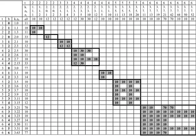
Combination of each of these 26 non-isomorphic branch configurations with those of the 24 value configurations enumerated before which are based on the same tip-configuration and prove non-isomorphic given the branch tip-configuration in question then yields the isomorphism classes of all (reduced-form) matrimonial rings consisting entirely of tips (or equivalently, of all the tip-parts of matrimonial rings within the chosen bounds). In our case of k ≤ 3, the derivation of their automorphism groups from those of the constituent branch- and value-configurations is largely facilitated by the fact that no groups other than the maximal groups have proper subgroups, so that the intersection of any two different non-maximal groups is the identity group. Since no configured matrimonial ring can have a maximal automorphism group (the condition of opposite values for edge-adjacent nodes makes at least one reflection impossible), none of the resulting automorphism group has proper subgroups. Table 2 lists the symmetry indices for all non-isomorphic tip-parts of matrimonial rings for k ≤ 3. There are 80 such configurations (3 for k = 1, 16 for k = 2 and 61 for k = 3):

t 2 2 2 2 3 3 4 4 4 4 4 4 5 5 5 5 6 6 6 6 6 6 6 6 k. zb. zv 1. 1. 1 1. 1. 2 2. 0. 1 2. 0. 2 2. 1. 3 2. 1. 4 2. 3. 3 2. 3. 5 2. 3. 10 2. 3. 12 3. 1. 5 3. 1. 10 3. 5. 11 3. 5. 13 3. 5. 18 3. 5. 20 3. 7. 11 3. 7. 13 3. 7. 19 3. 7. 21 3. 7. 42 3. 7. 44 3. 7. 50 3. 7. 52 t b k.zb ab 10 10 12 12 12 12 12 30 30 12 10 10 10 10 10 10 10 10 10 70 70 10 10 10 1 0 1.0 11 2 1 1.1 10 10 10 2 2 1.3 11 10 2 0 2.0 33 12 3 1 2.1 10 10 10 3 2 2.3 12 12 12 4 2 2.5 30 10 30 30 4 2 2.6 11 10 10 4 3 2.7 10 10 10 10 10 4 4 2.15 33 12 30 3 0 3.0 77 4 1 3.1 10 10 10 4 2 3.3 14 10 5 2 3.5 10 10 10 10 10 5 2 3.6 12 10 10 5 3 3.7 10 10 10 10 10 5 2 3.9 12 10 10 5 3 3.11 10 10 10 10 10 5 4 3.15 12 10 10 6 3 3.21 70 10 10 70 70 6 3 3.22 10 10 10 10 10 10 10 10 10 6 4 3.23 10 10 10 10 10 10 10 10 10 6 4 3.27 14 10 10 10 10 6 4 3.30 11 10 10 10 10 6 5 3.31 10 10 10 10 10 10 10 10 10 6 6 3.63 77 10 10 10 70

Table 2. Isomorphism classes of the tip-parts of matrimonial rings within bounds (3,2) Having thus determined all non-isomorphic configurations of the married individuals in a matrimonial ring, let us now look at the linking individuals, to begin with their number. Given a maximum depth of δ, each of the b branches may contain up

(15)

to δ - 1 linknodes. If we let bl be the number of branches with length l + 1 (l = 0, …, δ),

the total number of linknodes is h=

∑

δ_l₌₀h_l⋅l (which reduces to h = h1 for δ = 2). For each of the 79 configurations, the number of isomorphism classes of matrimonial rings containing hl branches of length l + 1 (in semi-neutral form, i.e., without yet determining the values of the linknodes) is given by the coefficient of the summand

1 2 1 1 2 1hxh ...xνhν−−

x in the polynomial obtained by substituting r r

r x x

s =1+ ₁ +...+ _ν₋₁ in the cycle index (b k)k

kab

Z + | _{. Multiplication of this polynomial with the number} b kab

N of

non-isomorphic tip-parts of rings with parameters k, b and ab (which is obtained by counting the appropriate cells of the Table 2) then counts the isomorphism classes of all matrimonial rings (in semi-neutral form) with parameters k, b and (hl) whose tip-part

has symmetry index ab. The resulting numbers still have to be decomposed according to the symmetry index of the complete (semi-neutral) ring. Now, since for k ≤ 3 no automorphism group of any configured tip-part has proper subgroups (cf. above), the symmetry index of the complete ring must either remain unchanged or reduce to the minimal symmetry index 10. It suffices therefore to inspect the branch-configurations of rings whose configured tip-parts have a non-minimal symmetry index, and count those which destroy the symmetry16_{. Summation over all l and all b then yields the numbers}

h kab

N of all isomorphism classes of (reduced semi-neutral) rings with h linknodes in k trees and symmetry index ab.

In the case of a reduced matrimonial universe (in which no matrimonial rings contain singular branches of length δ), calculation has to be modified. For k = 1, this can easily be done by reducing δ to δ – 1 for b = 1. For δ = 2 (where the restriction excludes any linknodes in singular branches), an alternative method consists in replacing b by 2(k – t + b) (the number of branches from branching roots).

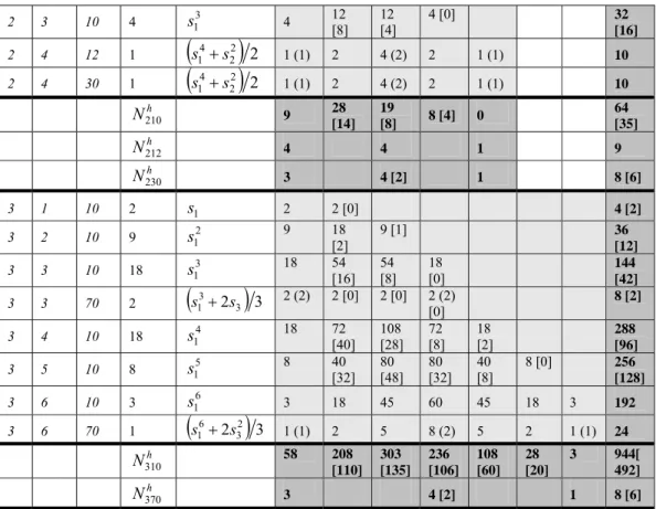
Table 3 contains the coefficients for the (3, 2)-universe. The number of symmetric structures (if they exist) is given in parenthesis, the numbers for the reduced universe (if they diverge) are given in brackets.

k b ab N_kabb Z_kab(b+k)|k h = 0 1 2 3 4 5 6 Σ 1 1 10 2 s₁ 2 2 [0] 4 [2] 1 2 10 1 s₁2 1 2 1 4 h N₁₁₀ 3 4 [2] 1 8 [6] 2 0 12 1 1 1 1 2 1 10 2 s₁ 2 2 [0] 4 [2] 2 2 10 3 s₁2 3 6 [0] 3 [0] 12 [3] 2 2 12 2

( )

2 1 2 1 + s 2 (2) 2 2 (2) 6 2 2 30 2

( )

s₁2+1 2 2 (2) 2 [0] 2 (2) _[0] 6 [2] _________________________

16_{For δ = 2, these are (with automorphism group index kab and total linknode number h in brackets]:} (1)1.(1)1 [30,0], (1)2.(1)2 [30,2], 1.1-1 [12,0], 1.2-2 [12,1], 1-1.1-1 [30,0],1-2.1-2 [30,2], 2-1.2-1 [30,2], 2-2.2-2 [30,4], 1-1.1-1 [12,0], 1-1.2-2 [12,2], 2-2.1-1 [12,2], 2-2.2-2 [12,2], (1)1.(1)1.(1)1 [70,0], (1)2.(1)2.(1)2 [70,3], 1-1.1-1.1-1 [70,0], 1-2.1-2.1-2 [70,3],2-1.2-1.2-1 [70,3], 2-2.2-2.2-2 [70,6].

(16)

3 6 1 s s + 1 (1) 2 5 8 (2) 5 2 1 (1) 24 h N₃₁₀ 58 208 [110] 303 [135] 236 [106] 108 [60] 28 [20] 3 944[ 492] h N₃₇₀ 3 4 [2] 1 8 [6]

Table 3. Enumeration of matrimonial ring types in semi-neutral form within bounds (3,2)

The final step consists in substituting r

r x

s =1+ into the weighted cycle index

b k n kab h kab Z

N ⋅ | + _{to obtain the numbers of all isomorphism classes of matrimonial rings with}

h linknodes in k trees and symmetry index ab. The coefficient of the summand xg_counts

the isomorphism classes of matrimonial rings containing g same-sex linknodes. Summing over all g, h and ab then gives the total number of isomorphism classes of matrimonial rings with given k and δ. They are given in Table 4:

k h ab N_kabh Zkabn|k+b g = 0 1 2 3 4 5 6 Σ 1 0 10 3 1 3 3 1 1 10 4 [2] s₁ 4 [2] 4 [2] 8 [4] 1 2 10 1 s₁2 1 2 1 4 8 [6] 6 [4] 1 15 [11] 2 0 10 10 1 9 9 2 0 12 3 1 4 4 2 0 30 3 1 3 3 2 1 10 28 [14] s1 28 _[14] 28 _[14] 56 [28] 2 2 10 19 [8] s₁2 19 _[8] 38 _[16] 19 _[8] 76 [32]

(17)

3 1 2 5 8 5 2 1 24 952 [498] 2118 [106 0] 1993 [106 5] 1020 [616] 298 [210] 48 [40] 4 6433 [3493]

Table 4. Enumeration of matrimonial ring types within bounds (2,3)

Within the bounds of up to three affinally linked consanguineous “families”, each delimited by first degree cousinhood, and without differentiating between full-sibling and half-sibling ties, there are thus 15 consanguineous marriage structures (k = 1), 256 classes relinking marriage structures with two families involved (k = 2), and 6433 relinking marriage structures with three families involved (k = 3). If apical ancestors of generational level δ are only considered as representations of a sibling tie, these numbers reduce to 11, 146 and 3493, respectively.

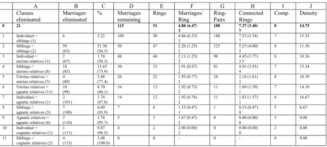
Appendix 1 gives an analytical overview of the (reduced) (2, 2)-universe, containing 11 consanguineous marriages and 146 relinking marriages. Each matrimonial ring type is represented by the ring with the lowest branch and value configuration numbers17. We have listed the rings both in conventional and in HF-notation, together with the indices of their most important structural characteristics (configuration numbers, symmetry indices, skewedness, agnatic and uterine degrees, length, width, depth, and the numbers of tips, linknodes, singular and non-singular branches and singular and branching roots).

_________________________

17_{We have assigned number zero to the ring H.F, since it is an open question among anthropologists} whether a remarriage with a former wife constitutes a proper relinking marriage or not.

(18)

3. THE MATRIMONIAL CENSUS

Having established a set of matrimonial ring types, we now turn to the question of analysing their distribution and mutual interconnection in empirical kinship networks. To this purpose, we first introduce some additional conceptual tools (Box 5):

Box 5. Matrimonial Census

Let K be a kinship graph with edge set M and a matrimonial universe U of extension µ. We define the elementary marriage type Mh ⊆ M (h = 1,…, µ) as the set of all edges in K which form part of a matrimonial ring of type h18_{. Let T}*

U(K) be the set of all elementary marriage types in K with respect to U.

Let M0 be the set of all marriage edges which do not enter in a matrimonial ring of any type from U. A marriage type in general is every subset of M which can be represented as the union, the intersection or the complement in M\M0 of elementary marriage types. The set TU of all marriage types constitutes a

topology (the matrimonial topology) onM\M0.

Let mh = |Mh| be the number of all elementary marriages of type h in K. The vector (mh) is called the

matrimonial census of K with respect to U (or briefly the (κ, δ)-matrimonial census of K if U is the maximal (κ, δ)-universe).

The census graph of K with respect to U is a 2-mode graph consisting of M and T*_{as node sets, and}

an arc from a node in T*_{(representing an elementary marriage type) to a node in M (representing a}

marriage edge) if the edge belongs to that type.

The 1-mode reduction of this census graph (or briefly the corresponding second order or 1-mode-census graph) is a valued graph with node set T*_{, where any two nodes are linked by an edge if they are}

partner nodes in the corresponding 2-mode census graph (in other words if the corresponding marriage types have a non-empty intersection), and the edge value corresponds to the number of nodes from M which are adjacent from both (i.e., to the extension of the combined marriage type resulting from the intersection of the two elementary types).

3.1 ESTABLISHING A MATRIMONIAL CENSUS BY MEANS OF pajek

The first step in the analysis of a matrimonial ring structure consists in establishing the matrimonial census of the kinship network under consideration. This entails (1) identifying all distinct matrimonial rings in the network (i.e., all rings that do not contain the same nodes), (2) assigning them to their appropriate isomorphism class and (3) counting the number of marriages which form part of a ring belonging to each class, i.e., in establishing the matrimonial census of the kinship network in question.

A powerful computer tool for doing that is the program PAJEK, developed by A. Mrvar and V. Batagelj (University of Ljubljana) for the explorative analysis of large networks [Batagelj and Mrvar, 2003; de Nooy et al., forthcoming])19. PAJEK contains a function which makes it possible to scan a given graph G1 for all induced subgraphs20

_________________________

18_{Note that this definition does not differentiate marriages according to their position in the matrimonial} ring (for instance, marriage with WD and WM, while quite different from Ego’s point of view, will be considered of the same “marriage type”, as they are part of a ring of the same type). A refined classification of marriage types would have to take into account not only the cycle passing through the marriage edge, but also of the path (other than that edge) which connects its two incident nodes.

19_{We have been using version 1.01f.}

20_{There is also the option in}_PAJEK_{to restrict the scan to those subgraphs of G1 which are identical to the} induced subgraphs generated by their node sets. In our case, this excludes all matrimonial rings which contain still smaller rings (i.e., whose nodes are linked to each other by lines which form not part of the ring). This option proves especially useful in the search for “pure” relinking marriages which are not at the same time consanguineous marriages (while, from Theorem 2 in Section 1.2, every consanguineous marriage is also a relinking marriage if the graph is regular and canonical in its neighbourhood).

(19)

(“fragments”) which are isomorphic to a given second graph G2, and to repeat this

fragment search for an arbitrary number of times, where G1 or G2 may be fixed. As a

by-product of each fragment search, PAJEK extracts a subgraph G12 from G1 by eliminating

all lines which are not contained in a fragment isomorphic to G2. If the fragment search

is repeated n times, PAJEK creates a vector which contains the n numbers of found fragments. These vectors can be saved as VEC-files (or TXT-files) and read in EXCEL or similar programs.

Applying this tool to establish the matrimonial census for a matrimonial universe of extension µ is straightforward. Having previously defined a set of µ abstract networks Gh (h = 3,…, µ + 2) each of which consists of a single matrimonial ring of a different class, and an additional network G2 consisting of a single marriage line (these

µ + 1 networks being saved and loaded as a single PAJEK project file), repeated scanning of a kinship network G1 for fragments isomorphic to each of the µ matrimonial rings

generates the vector of ring frequencies in G1, and subsequent scanning of each of the

extracted subgraphs G1h for fragments isomorphic to G2 generates the vector of

elementary marriage type frequencies, i.e., the matrimonial census.

Because PAJEK fragment searches check line values but not node values, all information on nodes has to be incorporated into the lines. This is done by transforming the original k-graph (which is a configured mixed graph) into a non-configured multigraph with 5 classes of arcs, such that each edge of the k-graph corresponds to an arc of class 1 (pointing from female to male node), and each arc of the k-graph connecting a node-pair with values (x1, x2) corresponds to an arc of class 2(x1 + 1) + x2

(x1, x2 ∈ {0, 1})21. We shall call this graph a k5-graph. Transformation of a k-graph into a k5-graph is accomplished by transformer programs like GEN2PAJEK, developed

especially for the present purpose by Jürgen Pfeffer (FAS.research, Vienna)22.

So as to be able to search for matrimonial rings in reduced form, it is further necessary to add a 6th class consisting of sibling edges for all sibling nodes in the original k-graph. As PAJEK contains a function for the addition of sibling edges, this can be easily done from the k5-graph by means of a short series of commands available as a

macro M123.

The (reduced) matrimonial universes with bounds (1, 4)24 and [2, 2] – containing 239 consanguineous marriage types and 146 relinking marriage types – have been _________________________

21_{This means that arcs belong to classes 2, 3, 4 and 5 according as they point from mother to daughter,} from mother to son, from father to daughter and from father to son. This coding makes it easy to shrink the network to the corresponding network of matri- or patri-“lineages” (the weak components of the graph which results from it by retaining only lines with values 2 and 3 or 4 and 5, respectively) linked by arcs that point from wife-giving to wife-taking lineages, as it is accomplished by the macros M5ab of the program package “pajek matrimonial census”.

22

GEN2PAJEK (to be downloaded at http://eclectic.ss.uci.edu/download/MarriageNetTools.htm) reads an EXCEL .XLS file whose columns are, for each individual: ID number, name, sex (H/F or H/M), father's ID number, mother's ID number and spouse's ID number (each of the individual's spouses are placed in a separate row). It generates a PAJEK .NET (network) file in which the original k-graph has been redefined as a k5-graph.

23_{All of the macros mentioned can be downloaded from the web at :}

http://eclectic.ss.uci.edu/download/MarriageNetTools.htm; the macros M2 and M3A used to generate census graphs are provided in Appendix 2.

24_{We shall not present the corresponding coefficient tables and ring lists for the (1,4)-universe here (it} contains the 239 types of consanguineous marriage structures within the bounds of third cousinhood).

(20)

defined as PAJEK-project files and can be downloaded from the web at

http://eclectic.ss.uci.edu/download/MarriageNetTools.htm. All census graphs which we

shall present as examples in the remainder of this paper have been generated with reference to these two universes.

Figures 3(a) and 3(b) show two examples of a matrimonial census generated by PAJEK: Figure 3(a) shows the (1,4)-census for the West African Jafun Fulani (503 marriages, 180 of them in 385 consanguineous rings belonging to 83 types), (cf. [Barry, 1996, 1998, 2000]); and for the Amerindian Chimane (747 marriages, 252 of them in 844 consanguineous rings belonging to 51 types, (cf. [Daillant, 2003]), together with the census for a random kinship network25. Figure 3(b) shows the (2,2)-census for the families of the European city of Ragusa from the XIIth to the XVIth century (2002 marriages, 490 of them in 587 2-family-relinking rings belonging to 91 types; a PAJEK sample genealogy, cf. [Mahnken 1960]) and for the Australian Aboriginal Nyungar (338 marriages, 115 of them in 151 2-family-relinking rings belonging to 51 types, (cf. [Tilbrook, 1983]), both of whom avoid close kin marriage. Here also, the census for a random kinship network has been added for comparison26. The data, presented graphically by means of EXCEL and expressed as percentages of the total number of marriages in each sample corpus, derives from the .VEC (vector) files generated as a by-product of PAJEK fragment searches. It is clear that while, in general, certain ring types (e.g., marriages between first cousins) occur more frequently than others (e.g., marriages between siblings), there are nonetheless significant differences in the distribution of frequencies from one network to the next.

______________________________________________________________________ They can be easily generated without consideration of symmetry properties, since each of the three possible valued tip-configurations for k = 1 is perfectly asymmetric. The complete table of the 239 consanguineous ring types (analogous to the one provided in appendix 1 for 146 relinking ring types) is available from the authors.

25_{The random network has been generated by G}

ENEORND 0.3. It contains 10.000 individuals, of which 2 % belong to the first generation. Men and women are uniformly distributed, annual death and divorce probability is 2 %, annual marriage probability (including polygamous marriages) is 10 %, annual reproduction probability 30 %. Women have children from 15 to 55 years, men from 20 to 60 years, the life span is 60 years for both sexes. The network contains 3501 marriages.

26_{The second random network has been generated under the same assumptions as the first, with the only} difference that 10 % of all individuals belong to the first generation. It contains 3209 marriages.

(21)

1 8 15 ₂₂ 29 ₃₆ 43 ₅₀ 57 ₆₄ 71 ₇₈ 85 ₉₂ 99 106 ₁₁₃ 120 ₁₂₇ 134 ₁₄₁ 148 ₁₅₅ 162 ₁₆₉ 176 ₁₈₃ 190 ₁₉₇ 204 211 ₂₁₈ 225 ₂₃₂ 239 Random Peul Chimane 0% 2% 4% 6% 8% 10% 12% Figure 3(a) 1 ₇ 13 ₁₉ 25 ₃₁ 37 ₄₃ 49 ₅₅ 61 ₆₇ 73 ₇₉ 85 ₉₁ 97 103 ₁₀₉ 115 ₁₂₁ 127 ₁₃₃ 139 ₁₄₅ Random Ragusa Nyungar 0% 2% 4% 6% 8% 10% 12% Figure 3(b)