HAL Id: hal-02929158
https://hal.archives-ouvertes.fr/hal-02929158
Submitted on 27 Oct 2020
HAL is a multi-disciplinary open access
archive for the deposit and dissemination of
sci-entific research documents, whether they are
pub-lished or not. The documents may come from
teaching and research institutions in France or
abroad, or from public or private research centers.
L’archive ouverte pluridisciplinaire HAL, est
destinée au dépôt et à la diffusion de documents
scientifiques de niveau recherche, publiés ou non,
émanant des établissements d’enseignement et de
recherche français ou étrangers, des laboratoires
publics ou privés.
combustion
R.J. Andres, T. Boden, F.-M. Bréon, P. Ciais, S. Davis, D. Erickson, J. Gregg,
A. Jacobson, G. Marland, J. Miller, et al.
To cite this version:
R.J. Andres, T. Boden, F.-M. Bréon, P. Ciais, S. Davis, et al.. A synthesis of carbon dioxide emissions
from fossil-fuel combustion. Biogeosciences, European Geosciences Union, 2012, 9 (5), pp.1845-1871.
�10.5194/bg-9-1845-2012�. �hal-02929158�
Biogeosciences, 9, 1845–1871, 2012 www.biogeosciences.net/9/1845/2012/ doi:10.5194/bg-9-1845-2012
© Author(s) 2012. CC Attribution 3.0 License.
Biogeosciences
A synthesis of carbon dioxide emissions from fossil-fuel combustion
R. J. Andres1, T. A. Boden1, F.-M. Br´eon2, P. Ciais3, S. Davis4, D. Erickson5, J. S. Gregg6, A. Jacobson7,8, G. Marland9, J. Miller7,8, T. Oda7,10, J. G. J. Olivier11, M. R. Raupach12, P. Rayner13, and K. Treanton14
1Environmental Sciences Division, Oak Ridge National Laboratory, Oak Ridge, TN 37831-6290 USA 2CEA/DSM/LSCE, Gif sur Yvette, France
3IPSL-LSCE, Gif sur Yvette, France
4Carnegie Institution of Washington, Stanford University, Stanford, CA 94305 USA
5Computational Earth Sciences Group, Computer Science and Mathematics Division, Oak Ridge National Laboratory, Oak Ridge, TN 37831 USA
6Risø DTU National Laboratory for Sustainable Energy, 4000 Roskilde, Denmark 7NOAA Earth System Research Lab, Boulder, Colorado 80305 USA
8Cooperative Institute for Research in Environmental Science, University of Colorado, Boulder, Colorado 80303 USA 9Research Institute for Environment, Energy, and Economics, Appalachian State University, Boone, NC 28608 USA 10Cooperative Institute for Research in the Atmosphere, Colorado State University, Fort Collins, Colorado 80523 USA 11PBL Netherlands Environmental Assessment Agency, Bilthoven, The Netherlands
12CSIRO Marine and Atmospheric Research, Australia
13School of Earth Sciences, University of Melbourne, Australia
14Energy Statistics Division, International Energy Agency, Paris, France
Correspondence to: R. J. Andres (andresrj@ornl.gov)
Received: 28 November 2011 – Published in Biogeosciences Discuss.: 31 January 2012 Revised: 17 April 2012 – Accepted: 24 April 2012 – Published: 25 May 2012
Abstract. This synthesis discusses the emissions of carbon
dioxide from fossil-fuel combustion and cement production. While much is known about these emissions, there is still much that is unknown about the details surrounding these emissions. This synthesis explores our knowledge of these emissions in terms of why there is concern about them; how they are calculated; the major global efforts on inventory-ing them; their global, regional, and national totals at differ-ent spatial and temporal scales; how they are distributed on global grids (i.e., maps); how they are transported in mod-els; and the uncertainties associated with these different as-pects of the emissions. The magnitude of emissions from the combustion of fossil fuels has been almost continuously in-creasing with time since fossil fuels were first used by hu-mans. Despite events in some nations specifically designed to reduce emissions, or which have had emissions reduction as a byproduct of other events, global total emissions con-tinue their general increase with time. Global total fossil-fuel carbon dioxide emissions are known to within 10 % un-certainty (95 % confidence interval). Unun-certainty on
individ-ual national total fossil-fuel carbon dioxide emissions range from a few percent to more than 50 %. This manuscript con-cludes that carbon dioxide emissions from fossil-fuel com-bustion continue to increase with time and that while much is known about the overall characteristics of these emissions, much is still to be learned about the detailed characteristics of these emissions.
1 Introduction
Emissions to the atmosphere of carbon dioxide (CO2)from fossil-fuel combustion are of concern because of their grow-ing magnitude, the resultgrow-ing increase in atmospheric concen-trations of CO2, the concomitant changes in climate, and the direct impact of increased atmospheric CO2 on ecosys-tems and energy demand. These ecosystem and climatic changes could adversely impact human society. This syn-thesis of information on fossil-fuel CO2 (FFCO2) emis-sions to the atmosphere is intended to summarize our current
understanding about FFCO2 emissions to the atmosphere in support of the Regional Carbon Cycle Assessment and Pro-cesses project (RECCAP, http://www.globalcarbonproject. org/reccap). After introductory remarks, this synthesis in-cludes a discussion of the different efforts to estimate global emissions (Sect. 2), an examination of the magnitude of global FFCO2 emissions (Sect. 3), the regional distribution (Sect. 4), national FFCO2 inventories (Sect. 5), the distribu-tion of FFCO2 over space and time (Sects. 5.1, 5.2, and 6), issues related to FFCO2 transport in the atmosphere (Sect. 7), and uncertainties involved in estimates of FFCO2 emissions (Sect. 8).
FFCO2 inventories, created by an accounting of FFCO2 emissions per unit of time, have at their core a measure of the amount and type of fossil fuels consumed over a given time interval. Different inventories have different foci. Some are more focused on fuel production while others on fuel consumption. Some contain details about the sectors of the economy in which fuels are consumed while others focus on the type of fuel. Some attempt to survey all nations of the world while others focus on only certain nations. Some focus on emissions within national borders while others on emis-sions outside these borders (e.g., transoceanic shipping and aircraft or the emissions embodied in trade). Inventories can be focused on specific geographic areas or on particular in-dustries, projects, products, activities, or time periods. Emis-sion inventories serve a variety of objectives and can differ significantly with the myriad of scientific and sustainability questions posed. Thus, comparisons between inventories are not always straightforward.
The more complete inventories contain FFCO2 emissions from the three major fossil fuels: solid fuels (e.g., coal), liq-uid fuels (e.g., petroleum), and gaseous fuels (e.g., natural gas). Added to these inventories may be CO2emissions from natural gas flaring and CO2 emissions from cement man-ufacture. Flaring of natural gas occurs as a byproduct of petroleum and natural gas extraction and processing. In oil fields that are not well connected to natural gas markets, for example, the co-produced natural gas is often burned at the well head because it is too expensive to capture and trans-port to market or re-inject into the ground. In areas deemed non-hazardous to humans, co-produced natural gas may also be vented instead of flared and these vented FFCO2 emis-sions are included as though they had been flared (an excep-tion is EDGAR 4.2 which only tracks flaring for most coun-tries (Olivier and Janssens-Maenhout, 2011)). No economic profit is made from this practice beyond avoiding costs asso-ciated with gas transport to market or re-injection. Cement manufacture is the process of converting calcium carbon-ate to lime with the CO2byproduct being emitted to the at-mosphere. Emissions from cement manufacture include only those from the carbonate to lime reaction (the emissions from burning fossil fuels to support this process are reported with the respective fossil fuels). Emissions from cement manu-facture are often included because they are one of the largest,
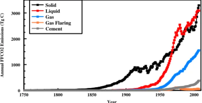
Fig. 1a. The contributions of five sources to FFCO2 emissions for the years 1751 to 2007. This figure was created from the sum of national production values (see section 1) for 15,830 country-year pairs (e.g., the United Kingdom in 1751 is the first country country-year pair, the United Kingdom in 1752 is the second country-year pair, and Zimbabwe in 2007 is the 15,830th country-year pair). The distribution of country-year pairs is generally increasing with time with the year 1751 containing one country-year pair and 2007 containing 216 country-year pairs. Data richness (e.g., the number of country-year pairs) is increasing with time due to increased energy data availability and the formal recognition of more countries (as there has been a general trend for larger countries to divide into smaller countries (e.g., former USSR)). In 2007, solid fuels accounted for 39% of the 2007 total, liquid fuels 37%, gas fuels 19%, gas flaring 1%, and cement 5% (percentages do not add to 100% due to rounding error). The unit of teragrams
carbon (Tg C) is equal to 1012 grams of carbon. To convert to Tg CO
2, multiply the total by the
molar ratios of carbon dioxide to carbon (44.0/12.0) or 3.67. Data from Boden et al. (2010).
Year
1750 1800 1850 1900 1950 2000
Annual FFCO2 Emissions (Tg C)
0 1000 2000 3000 Solid Liquid Gas Gas Flaring Cement
Fig. 1a. The contributions of five sources to FFCO2 emissions for
the years 1751 to 2007. This figure was created from the sum of na-tional production values (see Sect. 1) for 15 830 country-year pairs (e.g., the United Kingdom in 1751 is the first country year pair, the United Kingdom in 1752 is the second country-year pair, and Zim-babwe in 2007 is the 15 830th country-year pair). The distribution of country-year pairs is generally increasing with time with the year 1751 containing one country-year pair and 2007 containing 216 country-year pairs. Data richness (e.g., the number of country-year pairs) is increasing with time due to increased energy data availabil-ity and the formal recognition of more countries (as there has been a general trend for larger countries to divide into smaller countries (e.g., former USSR)). In 2007, solid fuels accounted for 39 % of the 2007 total, liquid fuels 37 %, gas fuels 19 %, gas flaring 1 %, and cement 5 % (percentages do not add to 100 % due to rounding er-ror). The unit of teragrams carbon (Tg C) is equal to 1012grams of carbon. To convert to Tg CO2, multiply the total by the molar ratios
of carbon dioxide to carbon (44.0/12.0) or 3.67. Data from Boden et al. (2010).
non-combustion, industrial sources of CO2to the atmosphere and there are good statistics worldwide on cement production rates. Cement manufacture inclusion in some FFCO2 inven-tories reflects the desire to have a more complete account-ing of anthropogenic emissions of CO2 to the atmosphere. Other industrial sources of CO2 to the atmosphere (e.g., as byproducts of acid production, steel production, etc.) are of-ten not included in FFCO2 inventories because of incomplete production statistics; their relatively smaller size compared to cement production; and because their individual magni-tude is generally smaller than the uncertainty associated with larger emissions from solid, liquid, and gaseous fuels. Fig-ure 1a shows one estimate of the contributions of these five major sources of FFCO2 to the atmosphere globally.
FFCO2 data are compiled from fossil-fuel production data or fossil-fuel consumption data. Production data are usually used for global totals as the uncertainty associated with pro-duction data is less than the uncertainty associated with con-sumption data. Reasons for the differences in uncertainty associated with production and consumption data are given later in this manuscript, but they generally fall into the cate-gories of fewer data points need to be collected for produc-tion values and these values are better known.
R. J. Andres et al.: A synthesis of carbon dioxide emissions 1847
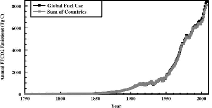
Fig. 1b. Comparison of FFCO2 emissions from global fuel use and the sum of countries for the years 1751 to 2007. This figure was created from the sum of national production and consumption values for 15,830 country-year pairs. Data from Boden et al. (2010).
Year
1750 1800 1850 1900 1950 2000
Annual FFCO2 Emissions (Tg C)
0 2000 4000 6000
8000 Global Fuel Use Sum of Countries
Fig. 1b. Comparison of FFCO2 emissions from global fuel use and
the sum of countries for the years 1751 to 2007. This figure was cre-ated from the sum of national production and consumption values for 15 830 country-year pairs. Data from Boden et al. (2010).
Consumption data are usually used for totals smaller than global (e.g., region, country, province/state, corporation) be-cause local specificity is needed to properly place fuel con-sumption in a particular area. This need for local specificity is removed when considering global totals. Fuel consumption is often not measured directly due to the lack of measure-ments (or statistics) at the appropriate spatial and temporal scales. Instead, fuel consumption is often inferred from esti-mates of apparent consumption where apparent consumption is defined as:
apparent consumption = 6(production + imports (1) −exports − bunkers − non − fuel uses − stock changes) where the summation is done for solid fuels, liquid fuels, gas fuels, gas flaring, and cement (Marland and Rotty, 1984). Bunker fuels are fuels used in international transport (e.g., shipping and aviation) and by international convention are not attributed to any one country. “Non-fuel uses” applies to fuels that are not consumed directly for energy (e.g., petroleum liquids to make plastics and asphalt or natural gas to make fertilizers). Stock changes occur when fuels are ac-cumulated or depleted in storage by producers, consumers, or shippers – usually in response to demand or price fluctua-tions. These additional terms are necessary to localize emis-sions statistics to a specific region as the location where a fuel is produced is often not the location where a fuel is con-sumed. Alternatively, FFCO2 emissions from specific end-uses (e.g., transport, homes, businesses, etc.) can also be es-timated from proxy data on fuel-consuming activities, such as vehicle kilometers driven or fuel receipts for heating.
The addition of these terms to calculate apparent consump-tion (hereafter referred to as consumpconsump-tion) creates more un-certainty in the consumption calculation as more detailed data from a larger number of fuel providers and consumers are needed. The collection of these more detailed data varies greatly, both in quality and quantity, between different coun-tries and regions. The need for collection of these more de-tailed statistics is obviated at the global scale because
im-ports should equal exim-ports; bunker fuels are consumed; stock changes are often assumed equal to zero because of the rel-atively small amount of stock changes compared to over-all fuel consumed annuover-ally (averaging less than 1 %, with a maximum of less than 3 %, of global totals for the years 1950–2007); and non-fuel uses are assumed equal to zero because over time these fuels are also eventually oxidized to CO2(at different rates for different uses).
As can be seen in Fig. 1b, the total of FFCO2 emis-sions from global fuel use (i.e., calculated from production data) does not equal FFCO2 emissions reported as the sum of emissions from all countries (i.e., calculated from con-sumption data). These two curves differ by a maximum of 400 Tg C in the year 2006 (5 % in that year) and an average of 24 Tg C (less than 1 %) over the 257-year record shown. The reasons for this discrepancy are fourfold: (1) bunker fu-els are included in the global totals, but not in the national totals; (2) non-fuel uses are included in the global totals, but not in national totals that include data on non-fuel energy consumption; (3) changes in stocks are assumed to be zero each year in the global totals, but are included in national to-tals when reported for individual countries; and (4) the sum of exports does not equal the sum of imports due to statistical errors and incomplete reporting. Bunker fuels are the largest source of difference between the FFCO2 from global totals and the sum of FFCO2 from all countries.
Accurate FFCO2 emissions inventories contribute knowl-edge to better understand the physical and economic environ-ment in which society exists and allow monitoring and verifi-cation efforts to reduce emissions. For example, via transport modeling (see Sect. 7), flux units of mass per time of FFCO2 inventories can be converted to the concentration units of CO2in the atmosphere (e.g., parts per million, ppm, Forster et al., 2007). On the physical environment side, FFCO2 in-ventories also help to understand: (1) the systematic trend of CO2concentration between northern and southern hemi-spheres (Denman et al., 2007); (2) the trend in stable car-bon isotopes of atmospheric CO2(δ13C, Ciais et al., 1995); (3) the trend in radiogenic carbon isotopes of atmospheric CO2 (114C, Levin et al., 2010); and (4) the trend in oxy-gen concentrations in the atmosphere (Keeling et al., 1993). FFCO2 emission inventories are consistent with these four atmospheric trends and are integral to their current explana-tion. On the economic side, FFCO2 inventories (particularly those with economic sectoral detail) also help to understand the relationships between fossil-fuel use and economic vital-ity (e.g., Olivier et al., 2011; IEA, 2010; Raupach et al., 2007; Bernstein and Roy, 2007; Levine and ¨Urge-Vorsatz, 2007; Ribeiro and Kobayashi, 2007; Kashiwagi, 1996; Michaelis, 1996). As it becomes increasingly apparent that the atmo-spheric concentration of CO2 needs to be limited, it is in-creasingly important to understand the sources of CO2, the activities and actors that are responsible for emissions, the success of mitigation efforts, and the extent to which the
many countries/parties are meeting their commitments to limit their emissions.
As this synthesis details, there are numerous methods for estimating CO2 emissions over space and time. In general, these emissions are attributed to the activities, regions, coun-tries, and time intervals over which they are produced (i.e., where and when fossil fuels are burned or otherwise used). However, fuels burned in one country may have been ex-tracted in another country and the resulting goods consumed in yet another country. In such cases, attribution of all emis-sions to the countries where the fuels are burned neglects the role of the countries extracting and exporting fossil fuels as well as the countries that either consume goods produced elsewhere or produce goods to be consumed elsewhere. Re-cent publications have quantified the lateral fluxes of fossil fuels transported internationally before being burned (Davis et al., 2011), as well as the FFCO2 emissions embodied in goods traded internationally (Peters et al., 2011; Davis and Caldeira, 2010). A separate RECCAP synthesis (Peters and Davis, 2012) assesses this literature.
2 Different global data sets available
There are currently four organizations that produce system-atic, global, annual estimates of FFCO2 emissions: The Car-bon Dioxide Information Analysis Center (CDIAC, http:// cdiac.esd.ornl.gov), the International Energy Agency (IEA, http://www.iea.org), the Energy Information Administration of the United States (US) Department of Energy (EIA, http: //www.eia.doe.gov), and a joint effort of the Joint Research Centre of the European Commission and PBL Netherlands Environmental Assessment Agency (Emission Database for Global Atmospheric Research (EDGAR), http://edgar.jrc.ec. europa.eu). An additional data set, compiled by the United Nations Framework Convention on Climate Change (UN-FCCC), summarizes emissions data reported by signatory countries and covers many countries, in particular most of the industrialized countries with large emissions. In gen-eral all of the emission estimates within these inventories agree with each other, for both global and national emis-sions, within about ±5 % for developed countries and within about ±10 % for developing countries (which generally have less resources and commitment to data collection and report-ing). These compilations all rely on estimates of how much fuel is consumed, estimates of average carbon content of the fuels consumed, and estimates of the fraction of fuel con-sumption that results in actual oxidation (i.e., combustion) of each fuel commodity. The fuel oxidation term is impor-tant as it assumes immediate oxidation to FFCO2. This ig-nores kinetic and other chemical effects and becomes impor-tant when measured atmospheric carbon concentration data is compared to model output (see Enting et al., 2012 and ref-erences therein; Boucher et al., 2009). The four global data sets listed above experience a lag time between the current
calendar year and their latest year of reported data due to the time needed to collect, analyze, calculate, and report the various data involved. In an effort to report more recent cal-endar year data, data from the BP Statistical Review of World Energy have been used to estimate global FFCO2 emissions (e.g., LeQuere et al., 2009).
The four global emissions data sets start with energy data from different sources, but ultimately all of the data come from national or corporate surveys and reporting. Energy statistics compiled by the IEA and the United Nations Statis-tics Office (UNSO), for example, are now collected from many countries with a common survey form. Nonetheless, the various international statistics are subject to differences in emphases, categories, units, unit conversions and report-ing, data processreport-ing, and quality assurance within the host organizations. The international statistics compilers are also left to fill in the blanks when countries provide incomplete data or do not respond at all (a common occurrence in some African countries, for example). The completeness and qual-ity of data are extremely variable around the world and the uncertainty of the data is also variable. Nonetheless, the pro-duction, consumption, and trade of fossil fuels have great economic importance and at least some records are available back to the beginning of the industrial revolution. Using data from a variety of sources, CDIAC has assembled estimates of CO2emissions, by country, that are reasonably complete back to 1751 (Andres et al., 1999). Notably, more than half of cumulative fossil-fuel consumption globally has been since 1980 so that overall accuracy is dominated by data from the most recent years. Similarly, emissions are, and have always been, dominated by a small number of countries (currently 20 countries are responsible for about 80 % of global emis-sions) so that uncertainty on the global total is dominated by data from a small number of countries.
In general, the large global compilations of emissions es-timates rely on international compilations of energy data and global average emissions factors, whereas the estimates of emissions from individual countries are able to use local un-derstanding of data idiosyncrasies and locally focused emis-sions factors. The result is that the global data sets pro-duce estimates that should be uniform and comparable across countries and across time, but the individual country esti-mates may include details based on insights that are uniquely representative of the countries that produced them.
There have been several analyses that attempted system-atic comparison across these multiple data sets. For exam-ple, the IEA now routinely compares its estimates with those reported by the individual countries to the UNFCCC. They report that “for most Annex II countries, the two calcula-tions were within 5 %. For some EIT (economies in transi-tion) and non-Annex I countries, differences. . . were larger. In some of the countries the underlying energy data were different; suggesting that more work is needed on the col-lecting and reporting of energy statistics for these coun-tries” (OECD/IEA, 2010). Marland et al. (1999) pursued a
R. J. Andres et al.: A synthesis of carbon dioxide emissions 1849
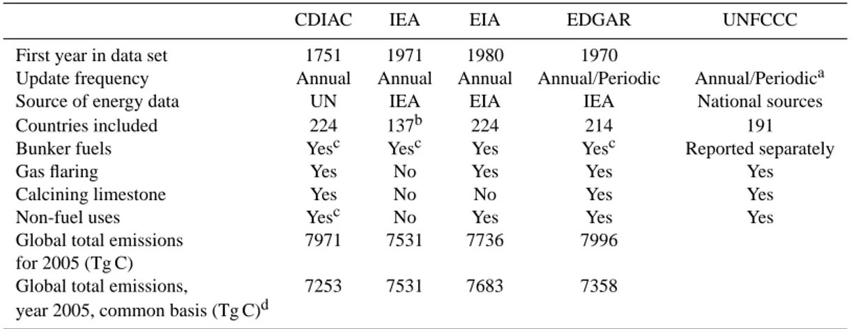
systematic comparison of the CDIAC and EDGAR data sets and Marland et al. (2007) reported a systematic comparison of estimates from CDIAC, EIA, and UNFCCC for the three countries of North America. Macknick (2009) has recently attempted a systematic comparison of four emissions data sets, and Ciais et al. (2010) have done a similar comparison for the countries of the European Union. A conclusion from these comparisons is that despite apparent similarity, there are differences in assumptions and boundary conditions that make it difficult to do quick quantitative comparisons. These differences result from, among other things, the inclusion of CO2from calcining limestone to make cement, the inclusion of emissions from fuels used in international transport, the treatment of fossil fuels that are used in non-fuel applica-tions, the treatment of natural gas flaring, and the treatment of fuels used for military purposes. Figure 2 and Table 1 sum-marize the published comparisons. This figure and table em-phasize some of the subtle differences in the different data sets. These differences are, of course, specifically character-ized in the documentation of each of the data sets, but their significance may not be readily apparent to data users.
Emissions reported annually by CDIAC are primarily de-rived from energy statistics published by the UNSO, which in turn reflect responses to United Nations (UN) and IEA questionnaires; official, national statistical publications; and the best estimates of the UNSO (Marland and Rotty, 1984; Andres et al., 1999; Boden et al., 2010). The total FFCO2 emissions reported in this manuscript are from fuel produc-tion data (see Sect. 1) and include, for each of 224 naproduc-tions or territories, emissions from bunker fuels (which for book-keeping purposes are allocated to the country where the fuels are loaded), natural gas flaring, calcining of limestone during cement production, and non-fuel uses.
Emissions reported annually by the IEA are primarily de-rived from sectoral energy statistics gathered by their own questionnaire, data sharing with the UNSO, official statis-tical publications, and the best estimates of the IEA staff. The IEA estimates global emissions using both a Tier 1 Sec-toral Approach and the Reference Approach following the methodology of the IPCC Guidelines for National Green-house Gas Inventories (IPCC, 1996). The IEA has chosen to use the Revised 1996 IPCC Guidelines based on advice from the UNFCCC since the Kyoto Protocol is based on this version of the Guidelines. This comparison is based on the Reference Approach calculations and is a modified version of the apparent consumption discussed in section 1 since the non-fuel uses are not subtracted from the apparent consump-tion, but an adjustment is made further along in the calcu-lation to exclude the non-fuel uses. The total FFCO2 emis-sions reported in this manuscript include, for each of 140 na-tions or regions, emissions from bunker fuels (bunker fuels are not included in national totals in IEA publications, but are shown separately by the IEA and included in their global totals). The IEA estimates do not include gas flaring,
calcin-Andres et al., FFCO2 Synthesis, p. 48/66
Fig. 2. Differences in total emissions reported by CDIAC, IEA, EIA, and EDGAR for 133 nations in 2007. The nations are spread along the y-axis according to their rank-order of mean FFCO2 emissions as reported in the respective data sets. Points near zero on the x-axis reflect small differences among the total emissions reported. Outliers reflect larger differences related to the disparate methodologies underlying reported emissions, for instance whether or not emissions from international bunker fuels and calcining of limestone are included.
Fig. 2. Differences in total emissions reported by CDIAC, IEA,
EIA, and EDGAR for 133 nations in 2007. The nations are spread along the y-axis according to their rank-order of mean FFCO2 emis-sions as reported in the respective data sets. Points near zero on the x-axis reflect small differences among the total emissions reported. Outliers reflect larger differences related to the disparate method-ologies underlying reported emissions, for instance whether or not emissions from international bunker fuels and calcining of lime-stone are included.
ing of limestone during cement production, nor non-fuel uses (OECD/IEA, 2010).
Emissions reported annually by the EIA are primarily de-rived from EIA-collected energy statistics from national sta-tistical reports. The EIA calculation methodology is similar to the CDIAC apparent consumption methodology, but the EIA uses internally generated carbon content and fraction oxidized coefficients. The total FFCO2 emissions reported in this manuscript include, for each of 224 nations or territo-ries, emissions from bunker fuels (which are allocated to the country where the fuels are loaded), natural gas flaring, and non-fuel uses. The EIA estimates do not include calcining of limestone during cement production (EIA, 2011a).
Emissions reported annually by the EDGAR effort are pri-marily derived from sectoral IEA energy statistics and default emission factors from the IPCC Guidelines (IPCC, 2006), and are presented in sectoral categories recommended by the IPCC (IPCC, 2006). The total FFCO2 emissions reported in this manuscript include, for each of 214 nations or territories, emissions from bunker fuels, natural gas flaring, calcining of limestone during cement production, and non-fuel uses us-ing the 2006 IPCC tier I methods (EC-JRC/PBL, 2011). The most recent full version of EDGAR (4.2) also reports other greenhouse gases.
The Parties to the UNFCCC are required to report period-ically on their GHG emissions. The 42 Parties that are listed in Annex I (industrialized nations and the European Union) are supposed to submit detailed emission reports annually; the 152 non-Annex I (developing nations) Parties less fre-quently submit less detailed reports as part of their National Communications. Submitted reports are calculated by the in-dividual Parties according to IPCC Guidelines (IPCC, 1996), and therefore include emissions from flaring of natural gas,
Table 1. Comparison of five global FFCO2 emissions inventories.
CDIAC IEA EIA EDGAR UNFCCC First year in data set 1751 1971 1980 1970
Update frequency Annual Annual Annual Annual/Periodic Annual/Periodica Source of energy data UN IEA EIA IEA National sources Countries included 224 137b 224 214 191 Bunker fuels Yesc Yesc Yes Yesc Reported separately
Gas flaring Yes No Yes Yes Yes
Calcining limestone Yes No No Yes Yes Non-fuel uses Yesc No Yes Yes Yes Global total emissions 7971 7531 7736 7996
for 2005 (Tg C)
Global total emissions, 7253 7531 7683 7358 year 2005, common basis (Tg C)d
aAnnex I countries are to report annually, non-Annex I countries have less stringent reporting requirements.
bDoes not include the three regions of Other Africa, Other Latin America, and Other Asia which contain data for countries not tabulated
separately.
cIn global totals, but not in national totals.
dCommon basis is an attempt to place all inventories on equal footing. Since the IEA is the least inclusive, their estimate was retained. EIA was
recalculated as the EIA value from the line above minus gas flaring (no separate tabulation for non-fuel hydrocarbons is listed). EDGAR was recalculated as the EDGAR value from the line above minus gas flaring minus cement minus non-fuel hydrocarbons. CDIAC was recalculated as the CDIAC value from the line above minus gas flaring minus cement minus non-fuel hydrocarbons.
calcining of limestone and other industrial processes, inter-national bunker fuels (as a memo item and not included in the national total) and non-fuel uses of fossil fuels. All data submissions are publicly available on the UNFCCC web-site (http://unfccc.int/ghg data/ghg data unfccc/items/4146. php).
The last data line of Table 1 is an attempt to place all of the inventories on a common basis. This was done by including only elements of the respective inventories common to all of them. In this regard, the IEA is the most restrictive so other inventories were modified to fit the IEA reporting categories as noted in Table 1. The average of the four values reported is 7457 Tg C with a standard deviation of 164 Tg C. On this common basis accounting, the three global data sets agree to within 3 % of their average. This agreement is considered remarkable when one understands their different accounting methods and starting data. See Sect. 8 for additional discus-sion about uncertainties associated with these data.
Due to the similarity of global data sets and the focus in this synthesis on the common message that these data sets provide, Sects. 3, 4, and 5 primarily use CDIAC data for the discussion development. Use of IEA, EIA, or EDGAR data would give similar results and/or conclusions. FFCO2 data reported in this manuscript are generally reported in mass carbon units; to calculate mass CO2units, multiply by 3.67 (the ratio of their molecular weights, 44/12).
3 Global FFCO2 emissions
3.1 Global FFCO2 emissions – the overall picture
Figure 3a shows the global magnitude of the annual FFCO2 emissions with time. The almost ever-increasing magnitude of the curve can be modeled by several equations. For exam-ple, a 10x2 Fourier Series polynomial fits the data extremely well although its terms do not have any known descriptive capability of relevant controlling processes. Only a slightly poorer fit is obtained by a simple exponential equation where its terms can be related to gross domestic product (GDP) and efficiency improvements (Raupach et al., 2008, 2007). How-ever, these equations fail to capture the short term decreases in year-to-year values when they occur (e.g., the 1930s de-pression, the 1945 end of World War II, the 1980s recession) and the year-to-year variability generally. Thus, for the his-torical record, the actual emission values are preferred in sci-entific studies. For projecting emissions into the near future, fit equations could be used (if one assumes the absence of major trend changes). For longer terms, projections are gen-erally based on assumptions regarding economic, technolog-ical, and population growth (e.g., Nakicenovic et al., 2000).
Figures 1a and 3a show that FFCO2 from each of the ma-jor fuel sources has grown over time. Coal was the domi-nant global energy source from 1750 to 1950 and contin-ues to grow in use. FFCO2 emissions from liquid fuels first surpassed those from coal in the late 1960s and now emis-sions from the two are similar (more than 3000 Tg C annu-ally). Increased global utilization of natural gas since 1950 is evident in the global FFCO2 record. Growth and economic development have resulted in increased cement production
R. J. Andres et al.: A synthesis of carbon dioxide emissionsAndres et al., FFCO2 Synthesis, p. 49/66 1851
Fig. 3a. Annual FFCO2 emissions for the years 1751 to 2007. This figure was created from the sum of national production values (see section 1) for 15,830 country-year pairs. Data from Boden et al. (2010). Year 1750 1800 1850 1900 1950 2000 A nnual FFC O2 Emissions (Tg C ) 0 2000 4000 6000 8000
Fig. 3a. Annual FFCO2 emissions for the years 1751 to 2007.
This figure was created from the sum of national production val-ues (see Sect. 1) for 15 830 country-year pairs. Data from Boden et al. (2010).
worldwide and, in turn, elevated releases of CO2from this anthropogenic source as well. A very recent trend is the increasing use of modern biofuels such as bioethanol and biodiesel to replace fossil oil products in road transport. Modern biofuels represented in 2009 and 2010 about 3 % of global road transport fuels (Olivier et al., 2011; Olivier and Peters, 2010). Although CO2emissions from biomass-based fuels are expected to continue increasing, they are not fossil fuels and thus not included in FFCO2 estimates.
Figure 3b shows the annual growth in FFCO2 emissions with time (i.e., the first derivative with respect to time of the curve in Fig. 3a). The importance of this figure is twofold: (1) despite variability, emissions are increasing with time (the average change is 33 Tg C per year over the 256 years shown), and (2) while the acceleration in emissions (i.e., the second derivative with respect to time of the curve in Fig. 3a, figure not shown) may appear visually to be increasing with time, statistically (p = 0.05 level) that acceleration is not sig-nificantly increasing with time. Instead, the large variabil-ity seen in more recent years of the time series is growing along with the overall magnitude of emissions (as seen in Fig. 3a). For example, the year 2003 to 2004 increase of nearly 400 Tg C represents less than 5 % of the 2004 total.
The cumulative emissions from FFCO2 activities are shown in Fig. 3c. From the year 1959 to the year 2008, an average of 43 % of these emissions remained in the atmo-sphere and were not removed by the terrestrial bioatmo-sphere or oceans (Le Qu´er´e et al., 2009). Rafelski et al. (2009) model this long term airborne fraction at 57 %. It is this transfer of carbon from geologic reservoirs to the atmosphere which is the primary driver of modern day concerns regarding cli-mate change. Figure 3c also highlights the sustained growth of FFCO2 emissions and that more than 50 % of FFCO2 has been emitted since 1980.
Table 2a shows the trends in individual national FFCO2 emissions over different time periods for countries that ex-isted with consistent statistics for the begin and end dates listed in the table. Note that some countries exist at the begin
Andres et al., FFCO2 Synthesis, p. 50/66
Fig. 3b. Growth of FFCO2 emissions from the year 1752 to 2007. Positive values indicate an increase in year-to-year emissions and negative values indicate a decrease in year-to-year emissions. A gray zero line has been added for reference. Data from Boden et al. (2010).
Year
1750 1800 1850 1900 1950 2000
Growth in Annual FFCO2 Emissions (Tg C/year)
-200 -100 0 100 200 300 400
Fig. 3b. Growth of FFCO2 emissions from the year 1752 to 2007.
Positive values indicate an increase in year-to-year emissions and negative values indicate a decrease in year-to-year emissions. A gray zero line has been added for reference. Data from Boden et al. (2010).
date but no longer exist at the end date (e.g., USSR, German Democratic Republic). Likewise, some countries exist at the end date but did not exist at the begin date (e.g., Czech Re-public, Ukraine). These countries which did not exist for the entire time period are excluded from the statistics in Table 2a. The statistics of Table 2a are sensitive to the end years cho-sen, but despite this, the significance of Table 2a is similar to that of Fig. 3a: emissions are increasing with time.
Note that growth is not universal as some of the growth factors are less than unity for some time intervals examined. Growth factors less than one indicate that FFCO2 emissions decreased with time over these time periods. For the begin date of 1950, only the Falkland Islands (Malvinas) had emis-sions that declined over this time interval. The Falkland Is-lands had extremely high per capita emissions in the early part of the time series which declined with time due to sig-nificantly reduced imports of refined oil. For the begin date of 1980, there are 25 countries who had reduced emissions over this time interval. These countries are located on five con-tinents. There are some notable features of these countries such as nine of them have made commitments/investments in non-fossil-fuel energy technologies such as nuclear power (e.g., France), six of them are former Soviet Union satellite countries (e.g., Hungary), four of them are in Africa (e.g., Gabon), and one has been under constant military engage-ments (i.e., Afghanistan). Note that despite these reductions in FFCO2 emissions in some countries, overall, the reduc-tions are small relative to global totals and the global to-tal (e.g., Fig. 3a) and global annual average growth (e.g., Fig. 3b) of FFCO2 emissions keeps increasing.
3.2 Global FFCO2 emissions – sectoral trends
When global FFCO2 emissions are examined by sector, power generation and industry dominate the total mass of emissions (Fig 3d). Since 1970, power generation and road
Fig. 3c. Cumulative FFCO2 emissions from the year 1751 to 2007. This figure was created from summing the data in Figure 3a. The dashed line indicates when approximately 50% of emissions have been emitted. Data from Boden et al. (2010).
Year 1750 1800 1850 1900 1950 2000 Cum u lative F F C O2 Em issions (Tg C) 0 50000 100000 150000 200000 250000 300000 350000
Fig. 3c. Cumulative FFCO2 emissions from the year 1751 to 2007.
This figure was created from summing the data in Fig. 3a. The dashed line indicates when approximately 50 % of emissions have been emitted. Data from Boden et al. (2010).
transport are the quickest growing sectors relative to their 1970 emissions.
These sectoral data are generated by the IEA and are a no-table feature of IEA and EDGAR data sets. Van Aardenne et al. (2001) have extended the EDGAR sectoral FFCO2 inven-tory back to 1890 for the main sectors.
Not shown in the aggregated data of Fig. 3d are the dif-ferences between mature industrialized countries and devel-oping countries. One notable change with time is the geo-graphical shift in emissions from the (manufacturing) try sector as it grows in developing countries while in indus-trialized countries it is increasingly replaced by the service sector (which is less fuel intensive).
3.3 Global FFCO2 emissions – through Kyoto eyes
Emission inventories allow us to ascertain the effectiveness of current international agreements that have the goal of “stabilization of greenhouse gas concentrations in the atmo-sphere at a level that would prevent dangerous anthropogenic interference with the climate system” (UNFCCC, 1992) by limiting emissions to the atmosphere. While the agreements do not focus solely on FFCO2 (KP, 1998), FFCO2 is a major component in obtaining treaty objectives. Furthermore, it is generally accepted that FFCO2 emissions must be reduced to stabilize atmospheric concentrations.
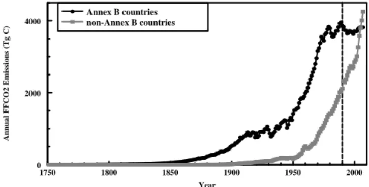
To examine the effect of these international agreements, figures similar to Fig. 3a, b, and c will be presented but with the data disaggregated by countries who have pledged treaty commitments (i.e., Annex B countries) and those who have not (i.e., non-Annex B countries). Most commitments are re-ductions below a baseline emission level, but not all commit-ments are reductions (KP, 1998).
Figure 3e is similar to Fig. 3a except that FFCO2 emis-sions are further categorized by Kyoto Protocol status. The black curve includes all countries who have pledged emis-sions limitations. The gray curve includes all countries where energy data and emission estimates exist but who have not
Fig. 3d. Sectoral FFCO2 emissions from the year 1970 to 2008. Data from EDGAR 4.2 (EC-JRC/PBL, 2011).
Year
1970 1980 1990 2000 2010
Annual FFCO2 Emissions (Tg C)
0 500 1000 1500 2000 2500 3000 3500 Power Generation Industry Road Transport Buildings Other Transport
Fig. 3d. Sectoral FFCO2 emissions from the year 1970 to 2008.
Data from EDGAR 4.2 (EC-JRC/PBL, 2011).
pledged emissions limitations. The curves cover years 1751 through 2007 and give a historical perspective to national emissions. The Kyoto Protocol years of interest include a 1990 base year with emissions limitations to be reached be-tween the years 2008 and 2012. These years are a subset of the data shown in Fig. 3e. Two important observations can be seen in Fig. 3e. First, regardless of Annex B status, and as with Fig. 3a, FFCO2 emissions are generally increasing with time. Second, the annual emissions from non-Annex B countries now exceed those from Annex B countries. This is in stark contrast to emission patterns when the Kyoto Proto-col was negotiated.
Figure 3f is similar to Fig. 3b except that FFCO2 emis-sions are further categorized by Kyoto Protocol status. The black curve includes all countries who have pledged emis-sions limitations. The gray curve includes all countries who have not pledged emissions limitations. Figure 3f shows the annual growth in FFCO2 emissions with time (i.e., the first derivative with respect to time of the curves in Fig. 3e). The importance of this figure is twofold: (1) despite variability, emissions are increasing with time (the average change over the 256 years shown in Fig. 3f is 15 Tg C per year for Annex B countries and 17 Tg C per year for non-Annex B countries), and (2) while the acceleration in emissions (i.e., the second derivative with respect to time of the curves in Fig. 3e, figure not shown) may appear visually to be increasing with time, statistically (p = 0.05 level) that acceleration is not signifi-cantly increasing with time. Instead, the large variability seen in more recent years of the time series is growing along with the overall magnitude of emissions (as seen in Fig. 3e), and much of the year-to-year variability is in non-Annex B coun-tries.
Figure 3g is similar to Fig. 3c except that cumulative FFCO2 emissions are further categorized by Kyoto Proto-col status. The black curve includes all countries that have pledged emissions limitations. The gray curve includes all countries who have not pledged emissions limitations. In terms of cumulative emissions, the Annex B countries have
R. J. Andres et al.: A synthesis of carbon dioxide emissions 1853 Andres et al., FFCO2 Synthesis, p. 53/66
Fig. 3e. Annual FFCO2 emissions for the years 1751 to 2007, disaggregated by Kyoto Protocol status. Similar to Figure 3a. This figure was created from the sum of national consumption values (see section 1) for 15,830 country-year pairs. For Yugoslavia and the USSR, two countries whose dissolution resulted in some states which signed the Kyoto Protocol and some states which did not sign, pre-dissolution emissions have been proportioned to the first year after dissolution. A dashed vertical line marks the Kyoto protocol base year of 1990. Data from Boden et al. (2010).
Year
1750 1800 1850 1900 1950 2000
Annual FFCO2 Emissions (Tg C)
0 2000 4000
Annex B countries non-Annex B countries
Fig. 3e. Annual FFCO2 emissions for the years 1751 to 2007,
disaggregated by Kyoto Protocol status. Similar to Fig. 3a. This figure was created from the sum of national consumption values (see Sect. 1) for 15 830 country-year pairs. For Yugoslavia and the USSR, two countries whose dissolution resulted in some states which signed the Kyoto Protocol and some states which did not sign, pre-dissolution emissions have been proportioned to the first year after dissolution. A dashed vertical line marks the Kyoto pro-tocol base year of 1990. Data from Boden et al. (2010).
emitted about 2.5 times more carbon to the atmosphere than the non-Annex B countries for the time period shown.
Table 2b shows the trends in individual national FFCO2 emissions from years 1990 to 2007 for Annex B and non-Annex B countries. For non-Annex B countries, the smallest growth factor is recorded for the Ukraine and likely reflects the faltering economy there. The largest growth factor is recorded for Spain with the 58 % growth well above their European Union internal burden-sharing agreement of 15 % growth (which is their national contribution to the overall Kyoto signed and ratified commitment of a European Com-munity 8 % reduction). The US, the largest FFCO2 emitter of the Annex B countries, has a growth factor of 1.20 (the 20 % increase is in contrast to the 7 % reduction commit-ment signed, but not ratified, in the Kyoto Protocol). The average of Annex-B countries is a 1 % reduction and given the increases over 1990 levels as seen in Fig. 3e, the Annex B countries are not on a linear track to meet their Kyoto tar-get of a 5 % GHG reduction by the 2008 to 2012 commit-ment period. However, using data that extends temporally beyond that in Fig. 3e to include the years 2008 and 2009 which includes the time of the global financial crisis, Olivier et al. (2011) conclude that the Annex B countries may meet their Kyoto target of a 5 % GHG reduction by the 2008 to 2012 commitment period. This summary excludes reductions in non-FFCO2 emissions and GHG reductions purchased from Clean Development Mechanism projects in non-Annex B countries, as allowed for by the Kyoto Protocol.
For non-Annex B countries (Table 2b), the smallest growth factor is recorded for the Republic of Moldova, and sim-ilar to the Ukraine above, this likely reflects the faltering economy. The largest growth factor is recorded for Namibia (495.63, although this may be a statistical aberration),
fol-Fig. 3f. Growth of FFCO2 emissions from the year 1752 to 2007, disaggregated by Kyoto Protocol status. Similar to Figure 3b. Positive values indicate an increase in year-to-year emissions and negative values indicate a decrease in year-to-year emissions. An orange zero line has been added for reference. Data from Boden et al. (2010).
Year
1750 1800 1850 1900 1950 2000
Growth in Annual FFCO2 Emissions (Tg C/year)
-200 -100 0 100 200 300 Annex B countries non-Annex B countries
Fig. 3f. Growth of FFCO2 emissions from the year 1752 to 2007,
disaggregated by Kyoto Protocol status. Similar to Fig. 3b. Positive values indicate an increase in year-to-year emissions and negative values indicate a decrease in year-to-year emissions. An orange zero line has been added for reference. Data from Boden et al. (2010).
lowed by Equatorial Guinea (40.07), Somalia (32.82), Cam-bodia (9.84), and Laos (6.60). China, a non-Annex B coun-try and the largest FFCO2 emitter in the world, has a growth factor of 2.66. The average growth for non-Annex B coun-tries is more than a 400 % increase (equal country weighted) and explains much of the large growth in emissions seen in Fig. 3a and e (with the majority of this growth from China on a mass-basis).
The important message from Table 2b is similar to the message of Fig. 3a: emissions are increasing with time. Note, again, this growth is not universal as a few growth factors are less than unity. These growth factors less than one indicate that 2007 FFCO2 emissions were less than FFCO2 emissions in 1990. There are 20 Annex-B countries with growth fac-tors less than one and 23 non-Annex B countries with growth factors less than one. While economic hardships can explain some of these growth factors, it is not the sole explanation. Deliberate policy actions have reduced FFCO2 emissions in some countries. Also, the reunification of Germany and the switch from coal to natural gas in the United Kingdom and Germany have resulted in decreases in FFCO2 emissions. Future policy actions may want to target the electricity gener-ation and the transport sectors for future FFCO2 reductions. The IEA Sectoral Approach shows that between 1971 and 2008, emissions from these sectors increased from one-half to two-thirds of total global emissions.
Figure 3e, f, and g and Table 2b give a sense of the annual, growth of, and cumulative FFCO2 emissions, subdivided by Kyoto Protocol status. Along with analogous Fig. 3a, b, and c, and Table 2a, these measures have been given as global to-tals because in terms of atmospheric radiative effects, it does not matter from which individual country emissions origi-nated. The mixing time of FFCO2 in the atmosphere is rela-tively short compared to its lifetime. Thus, it does not matter if a molecule of FFCO2 originates from the US, China, or Zimbabwe – its effect on atmospheric radiative effects is the
Fig. 3g. Cumulative FFCO2 emissions for years 1751 to 2007, disaggregated by Kyoto Protocol status. Similar to Figure 3c. This figure was created from summing the data in Figure 3e. Data from Boden et al. (2010).
Year
1750 1800 1850 1900 1950 2000
Cumulative FFCO2 Emissions (Tg C)
0 50000 100000 150000 200000 250000 Annex B countries non-Annex B countries
Fig. 3g. Cumulative FFCO2 emissions for years 1751 to 2007,
dis-aggregated by Kyoto Protocol status. Similar to Fig. 3c. This figure was created from summing the data in Fig. 3e. Data from Boden et al. (2010).
same. It is the total quantity of CO2in the atmosphere which is of ultimate concern to climate change processes.
Note that atmospheric CO2 concentration stands in con-trast to some other measures of FFCO2 properties. Carbon intensity is defined as the mass of FFCO2 emissions divided by a unit of GDP (EIA, 2011b, Raupach et al., 2007). By this measure, the US FFCO2 situation is improving as this ratio is decreasing. However, as GDP is generally increas-ing, this ratio masks the fact that FFCO2 emissions are also increasing. The decreasing ratio implies that the economy is operating more efficiently in terms of FFCO2 emissions. The decreasing ratio does not assure that absolute emissions are decreasing.
3.4 Global FFCO2 emissions – why care?
One can consider CO2 emissions not only in terms of an-nual fluxes but also as cumulative totals (e.g., Fig. 3c and g). One significance of cumulative emissions arises from the relationship between warming above preindustrial tempera-tures (T ) and cumulative anthropogenic CO2emissions (Q) from fossil-fuel combustion and net land use change since the start of the industrial revolution around 1750. Several recent papers have proposed that the relationship T (Q) is robust and quantifiable within uncertainty bands (Allen et al., 2009; Meinshausen et al., 2009; Zickfeld et al., 2009; Matthews et al., 2009; Raupach et al., 2011).
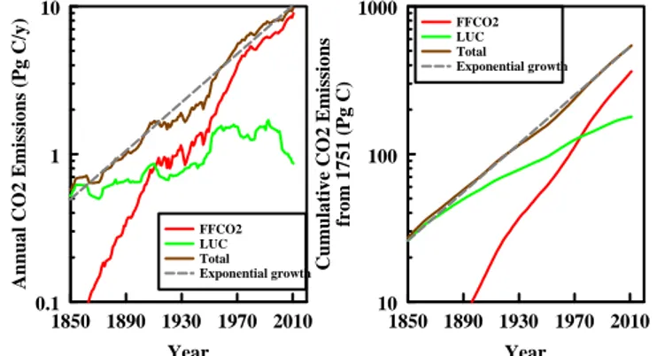
Figure 3h shows the history of annual emissions and cu-mulative emissions (since 1751) of FFCO2 and carbon emis-sions from land use change (LUC), together with their sum, the total CO2emissions from human activities. Annual emis-sions (left panel of Fig. 3h) are first considered. The past growth trajectories for FFCO2 and LUC emissions are differ-ent: LUC emissions have leveled off over the decades since around 1970 and have very likely decreased since around 2000 (Houghton et al., 2012), whereas FFCO2 emissions continue to increase strongly apart from a small recent dip attributable to the global financial crisis (Peters et al., 2011;
Fig. 3h. Annual and cumulative global CO2 emissions for years 1850 to 2007. Left panel:
Annual global CO2 emissions from fossil fuels and other industrial processes including cement
manufacture (FFCO2, red), land use change (LUC, green) and total (FFCO2 + LUC, brown).
Right panel: Cumulative global CO2 emissions from 1751, color coded as in left panel. Axes are
linear-log so that exponentially growing emissions appear as a straight line. In both panels, the FFCO2 is the same global fuel use data as displayed in Fig. 1b. In both panels, the dashed grey line is a fit to the total (FFCO2 + LUC) emissions data of an exponential-growth model with a growth rate of 1.9% per year. This corresponds to a doubling of emissions and cumulative
emissions every 37 years. The unit of petagrams carbon (Pg C) is equal to 1015 grams of carbon.
Year
1850 1890 1930 1970 2010
Cumulative CO2 Emissions
from 1751 (Pg C) 10 100 1000 FFCO2 LUC Total Exponential growth Year 1850 1890 1930 1970 2010
Annual CO2 Emissions (Pg C/y)
0.1 1 10 FFCO2 LUC Total Exponential growth
Fig. 3h. Annual and cumulative global CO2 emissions for years
1850 to 2007. Left panel: Annual global CO2emissions from fossil
fuels and other industrial processes including cement manufacture (FFCO2, red), land use change (LUC, green) and total (FFCO2 + LUC, brown). Right panel: Cumulative global CO2emissions from
1751, color coded as in left panel. Axes are linear-log so that expo-nentially growing emissions appear as a straight line. In both panels, the FFCO2 is the same global fuel use data as displayed in Fig. 1b. In both panels, the dashed grey line is a fit to the total (FFCO2 + LUC) emissions data of an exponential-growth model with a growth rate of 1.9 % per year. This corresponds to a doubling of emissions and cumulative emissions every 37 years. The unit of petagrams carbon (Pg C) is equal to 1015grams of carbon.
Friedlingstein et al. 2010; Le Qu´er´e et al. 2009). Combining both trajectories, the sum of FFCO2 and LUC emissions has grown almost exponentially, at 1.9 % per year (doubling time 37 yr), over the period 1850 to 2010.
The corresponding cumulative emissions are shown in the right panel of Fig. 3h. For more than 100 years, the to-tal (FFCO2 + LUC) cumulative emission has grown ex-ponentially at 1.9 % per year, like the annual total emis-sion. The scatter in the total cumulative emission about the exponential-growth line is much less than for annual emis-sions, because of the smoothing effect of accumulation. The total (FFCO2 + LUC) cumulative emission to the end of 2009 was about 530 Pg C, rising at nearly 10 Pg C per year (Le Qu´er´e et al. 2009). Of this total about 350 Pg C is due to FFCO2 and 180 Pg C to LUC, but the share of the cumulative total due to FFCO2 is increasing progressively.
4 Regional FFCO2 emissions
Disaggregating global FFCO2 emissions into regional emis-sions allows disaggregation of the global totals within the context of some regional specificity. From Fig. 4, it is seen that the largest emitting region has evolved over time from Western Europe (WEU) to North America (NAM) to Cen-trally Planned Asia (CPA). Other regions have risen and fallen relative to their peers over different time frames. For the entire 1751 to 2007 time series, the quantitative order of regional growth rates is mirrored by their qualitative order in
R. J. Andres et al.: A synthesis of carbon dioxide emissions 1855
Table 2a. Basic statistics regarding trends in normalized national
FFCO2 emissions for different time periods. n = number of coun-tries which existed at both the beginning and end dates, min = min-imum annual growth factor for the n countries (equal country weighted, not weighted by mass per country), med = median annual growth factor, avg = average annual growth factor, max = maximum annual growth factor. The growth factor is defined as the end date FFCO2 emissions divided by the begin date FFCO2 emissions. A factor of one indicates emissions were equal at the begin and end dates. A factor of two indicates that emissions doubled over the time period. It should be noted that available data for gas flaring and cement production vary by country. In some cases, inclusion of FFCO2 from these sources is sizable (e.g., gas flaring for Middle Eastern countries in the 1970s). Thus, growth factors may also re-flect new sources (e.g., there is no gas flaring data in 1900, but it does occur in many countries in 2007. Thus, the 1900–2007 growth factor statistics includes the addition of gas flaring.). Data from Bo-den et al. (2010).
Begin End n Min Med Avg Max Date Date
1900 2007 33 1.28 31.99 161.21 2469.23 1950 2007 126 0.21 18.19 43.71 403.08 1980 2007 175 0.27 2.16 3.29 82.24
2007 with CPA being the largest and Germany (GER) being the smallest. Different time periods could have dramatically different absolute and relative growth rates associated with them.
Regionally disaggregated emissions serve as essential in-puts to integrated assessment models (which can be used to examine the policy-economy-climate interrelationships). These models simulate global energy systems, resource con-sumption, and socioeconomic development scenarios for the next century for multi-country regions. Emissions are cali-brated to historical data and then simulated using different scenarios for the future (e.g., Belke et al., 2011; Sadorsky, 2011; Apergis and Payne, 2009).
The regional designations shown in Fig. 4 are a relic of Cold War politics and, to a lesser degree, of geopolitical and corresponding data reporting changes. While maybe not as politically relevant today, the historical UN regional defini-tions still serve the regional specificity purpose (e.g., NAM is North America and WEU is Western Europe). However, even WEU is not as clear as it could be. In 1994, CDIAC created a new regional entity, GER. GER incorporated the Federal Re-public of Germany (from WEU) and the German Democratic Republic (from Centrally Planned Europe, CPE). The re-united Germany did not fit easily within WEU or CPE. CPA, Centrally Planned Asia, is no longer a faithful description of China and Mongolia, but it still provides a useful grouping for examining the evolution of emissions over time.
Ultimately, one would want regional groupings that reflect something of importance to the task currently at hand (e.g., Fig. 3e, 3f, and 3g used Annex B and non-Annex B
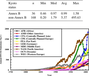
coun-Table 2b. Basic statistics regarding trends in normalized national
FFCO2 emissions for Annex B and non-Annex B countries from years 1990 to 2007. n = number of countries, min = minimum an-nual growth factor for the n countries (equal country weighted, not weighted by mass per country), med = median annual growth fac-tor, avg = average annual growth facfac-tor, max = maximum annual growth factor. The growth factor is defined as the year 2007 FFCO2 emissions divided by the year 1990 FFCO2 emissions. For some countries proportional emissions were used in 1990 or 2007 as the countries were disaggregated (e.g. former Soviet Union) or aggre-gated (e.g., Yemen). Thirteen non-Annex B countries (all relatively small FFCO2 emitters, the largest equal to less than 0.2 % of the sum of countries total FFCO2 emissions) were excluded from the analysis because the 1990 data year FFCO2 emissions data were incomplete or missing. Data from Boden et al. (2010).
Kyoto n Min Med Avg Max status
Annex B 36 0.46 0.97 0.99 1.58 non-Annex B 168 0.20 1.79 5.37 495.63
Fig. 4. Regional FFCO2 emissions for the years 1751 to 2007. This figure was created from the sum of national consumption values (see section 1) for 15,830 country-year pairs. See Boden et al. (2010) for which countries are included in each region. Data from Boden et al. (2010).
Year
1750 1800 1850 1900 1950 2000
Annual FFCO2 Emissions (Tg C)
0 500 1000 1500 2000 AFR (Africa) AMD (Other America) CPA (Centrally Planned Asia) CPE (Centrally Planned Europe) FEA (Far East)
GER (Germany) MDE (Middle East) NAM (North America) OCN (Oceania) WEU (Western Europe)
Fig. 4. Regional FFCO2 emissions for the years 1751 to 2007. This
figure was created from the sum of national consumption values (see Sect. 1) for 15 830 country-year pairs. See Boden et al. (2010) for which countries are included in each region. Data from Boden et al. (2010).
try groupings). No single description of regional groupings captures perfectly the geopolitical and economic changes in recent centuries. However, for the purposes of this synthesis, the historical CDIAC regional groupings serve as a useful example.
5 National FFCO2 emissions
National and annual FFCO2 emissions are the basic unit of global FFCO2 emissions. It is at national and annual scales that most energy statistical data are collected by national sta-tistical offices, agencies and/or energy ministries or amassed by centralized energy statistics efforts (e.g., UNSO). The richness and quality of national energy statistics have im-proved with time. These national and annual data are then
Fig. 5. Normalized national FFCO2 emissions for the years 1950 to 2007. This figure was created from the national consumption values (see section 1) and then normalized to 1950 emissions so that each country has a relative FFCO2 emission value equal to one in 1950. The U.S. curve lies nearly on top of that from the Falkland Islands. Data from Boden et al. (2010).
Year
1950 1960 1970 1980 1990 2000 2010
Normalized FFCO2 Emissions
0 100 200 300 400 500 Libya Grenada
Falkland Islands (Malvinas) USA
China
Fig. 5. Normalized national FFCO2 emissions for the years 1950 to
2007. This figure was created from the national consumption values (see Sect. 1) and then normalized to 1950 emissions so that each country has a relative FFCO2 emission value equal to one in 1950. The US curve lies nearly on top of that from the Falkland Islands. Data from Boden et al. (2010).
aggregated for regional (e.g., Sect. 4) or global (e.g., Sect. 3) summaries. These national and annual data can also play a role when looking at finer spatial (e.g., Sect. 5.1) and tempo-ral (e.g., Sect. 5.2) scales.
Figure 5 shows relative FFCO2 emission histories for five selected countries to illustrate some of the FFCO2 emission trajectories since 1950. These histories were each normal-ized to 1950 national FFCO2 emissions. Histories were con-structed from the 11 060 country-year pairs that exist in the data set from 1950 to 2007 which are distributed amongst 246 countries. Some countries were excluded from Fig. 5 for the following reasons: (1) they did not exist in 1950 (e.g., Azerbaijan, 86 countries total); (2) they did not exist in 2007 (e.g., USSR, 23 countries total); (3) they included incomplete or odd data during the years 1950 to 2007 (e.g., Botswana, six countries total); and (4) their 1950 FFCO2 emissions were less than 0.001 Tg C (e.g., Vanuatu, nine countries to-tal). These deletions left 122 countries for possible display in Fig. 5.
Figure 5 shows normalized data curves representing the full range of relative growth curves as well as some other fea-tures of the data. Libya has the largest relative growth over this time interval (from 39 Tg C in 1950 to 15 600 Tg C in 2007, a growth factor of 403). Grenada represents the av-erage relative growth over this time interval (from 1.7 Tg C in 1950 to 66 Tg C in 2007, a growth factor of 40). The Falkland Islands has the smallest relative growth over this time interval (from 75 Tg C in 1950 to 16 Tg C in 2007, a growth factor of 0.21). Two additional curves represent the two largest FFCO2 emitters in 2007. The curve for the US (from 692 124 Tg C in 1950 to 1 591 756 Tg C in 2007, a growth factor of 2) lies nearly on top of that from the Falk-land IsFalk-lands. The curve for China (from 21465 Tg C in 1950 to 1 783 029 Tg C in 2007, a growth factor of 83) lies slightly above that from Grenada.
Fig. 6a. Comparison of FFCO2 emissions from two CarbonTracker (CT) simulations for the CT Euarasia temperate region. FFCO2 emissions were revised and updated between the two CT simulations. Data from Jacobson (unpublished data).
Year 2000 2001 2002 2003 2004 2005 2006 2007 Annual FFCO2 Em is si ons (Tg C) 0 500 1000 1500 2000 2500 3000 CT2007B CT2007
Fig. 6a. Comparison of FFCO2 emissions from two CarbonTracker
(CT) simulations for the CT Euarasia temperate region. FFCO2 emissions were revised and updated between the two CT simula-tions. Data from Jacobson (unpublished data).
All the other 117 countries with complete data from 1950 to 2007 lie in between Libya and the Falkland Islands. Not all curves are monotonic as the bottom two curves suggest. Rather, some curves have strong departures from monotonic-ity as seen in the Libya curve.
While national and annual scale data are sufficient for many purposes, finer resolution data are often needed to pro-vide a process-based understanding of the global carbon cy-cle and to motivate and evaluate efforts to control FFCO2 emissions. General circulation models for climate change could utilize emissions data on a latitude-longitude grid at spatial resolutions much higher than that of nations. Flux in-version models benefit from much higher resolution of emis-sions than what is currently available in the national invento-ries (Gurney et al., 2002), to provide the best possible prior estimates, especially because FFCO2 emissions are usually held fixed in inversions (i.e., un-optimized, see Enting et al. (1995) for an exception to the usual practice). Addition-ally, high resolution data sets of emissions give more infor-mation on how specific human activities affect the carbon cy-cle and can allow for decision makers to better target the most economic ways to reduce emissions from human sources. The next two subsections of section 5 briefly discuss sub-national and sub-annual FFCO2 data sets.
5.1 Sub-national FFCO2 emissions
Data on sub-national (e.g., state, province, county, city, high-way, large point source) FFCO2 emissions are not very com-mon. Data at this level are usually collected for very specific purposes and may not be available for all types of fossil-fuel consumption. Such data are also not always made publicly available for commercial competitiveness reasons. Despite these restrictions, there are data available at the sub-national spatial scale for some countries. Oftentimes, these data are not as detailed or complete as the national data, but insights can be made. Section 6 of this paper describes efforts to dis-play FFCO2 emissions data on a latitude/longitude grid. This