Development of a light force accelerometer

Development of a Light Force Accelerometer

by

David LaGrange Butts

B.A, Williams College (2006)

Submitted to the Department of Aeronautics and Astronautics

in partial fulfillment of the requirements for the degree of

Master of Science in Aeronautics and Astronautics

at the

MASSACHUSETTS INSTITUTE OF TECHNOLOGY

May 2008

@

Massachusetts Institute of Technology 2008. All rights reserved.

A uthor ...

...

Department of Aeronautics and Astronautics

May 23, 2008

Certified by ...

Richard Stoner, Ph.D.

Principal Member of the Technical Staff

Thesis Supervisor

Certified by ...

Shaoul Ezekiel, Sc.D.

Professor of Aeronautics and Astronautics and

Electrical Engineering and Computer Science

Thesis Supervisor

Accepted by.

I-OCT

15 2008

LIBRARIES

David L. Darmofal

Associate Department Head

Chair, Committee on Graduate Students

ARCHIVES

v

Development of a Light Force Accelerometer

by

David LaGrange Butts

Submitted to the Department of Aeronautics and Astronautics on May 23, 2008, in partial fulfillment of the

requirements for the degree of

Master of Science in Aeronautics and Astronautics

Abstract

In this work, the feasibility of a light force accelerometer was experimentally demonstrated. The light force accelerometer is an optical inertial sensor which uses focused laser light to levitate and trap glass microspheres as proof masses. Acceleration is measured by force re-balancing, which is exerted by radiation pressure from two counter-propagating laser beams. Proof mass displacements are measured by focusing light scattered by the proof mass on a position-sensitive photodetector. A simple model including laser relative intensity noise and shot noise from the measurement of the trapping beam powers estimates that the light force accelerometer could be capable of achieving a sensitivity of < 100 ng/Hz1/2

Essential components of this optical accelerometer, including the levitation of 10 Pm glass microspheres in high vacuum and optical force rebalancing, were demonstrated with a single laser beam levitating a microsphere against gravity. Levitated particles are unstable in vacuum because of low viscous forces, so feedback stabilization is necessary for long term trapping. Preliminary performance diagnostics tested the short term sensitivity and bias stability of the apparatus for a constant 1 g acceleration. The factors currently limiting these performance parameters were determined to be bias instabilities associated with mea-surement of proof mass position and long term biases due to pressure-dependent radiometric effects.

Proposed modifications to the current apparatus include the implementation of a two-beam light force accelerometer and a more precise particle position detection method which is less sensitive to proof mass irregularities. This two-beam configuration enables operation in any orientation and permits complete characterization of accelerometer performance. Steps to develop a compact light force sensor in the future are also suggested.

Thesis Supervisor: Richard Stoner, Ph.D. Title: Principal Member of the Technical Staff Thesis Supervisor: Shaoul Ezekiel, Sc.D.

Title: Professor of Aeronautics and Astronautics and Electrical Engineering and Computer Science

Acknowledgments

I have been fortunate to spend the last two years working with some remarkably smart and talented people who have supported my work at MIT. I would like to thank Dr. Richard Stoner and Dr. Brian Timmons for their dedicated support, mentoring, and friendship. Rick's grasp of physics, sense of humor, and professionalism are something to aspire to, and it was a pleasure working together. Brian's generosity and supportive understanding of graduate school's trials added much needed levity to the demands of grad student life. I am also indebted to his knowledge of lab hardware and software, which saved me countless hours of frustration and contributed to much of the progress I made in this project. It was a blast to work in a lab with a great crew- Paul Jones, J.P. Laine, Jason Langseth, Jesse Tawney, and many others. I would also like to thank the Draper Laboratory for supporting my fellowship, providing me with challenging research, and surrounding me with high caliber people.

I would like to thank Prof. Shaoul Ezekiel for his valuable guidance in developing this work, and for making it fun to talk about experiments. I would like to acknowledge Prof. Jeffrey Hoffman for helping me make the most of my time at MIT and making the transition to engineering a smooth one.

To my friends at MIT- Robert Panish, Matt Abrahamson, Russell Sargent, Chris Mandy, Bobby Legge, and many others- it's hard to imagine being at MIT without all of you.

I am grateful for my loving parents and sister who have encouraged me to excel in everything I do. I am also thankful for the love and support of my fiance, Erika Latham, and to have spent many great weekends away from Cambridge with her family in Westhampton, MA. Finally, I would like to recognize my grandfather, Frank Regensburg, who passed away during my first year at MIT. His encouragement and passionate interest in my endeavors helped me get to where I am today.

This thesis was prepared at the Charles Stark Draper Laboratory, Inc., under the Precise Inertial Sensing Internal Research and Development Contract CON05001-2 Project ID 21806 Activity ID 001.

Publication of this thesis does not constitute approval by Draper or the sponsoring agency of the findings or conclusions contained herein. It is published for the exchange and stimulation of ideas.

Assignment

Draper Laboratory Report Number T-1609.

In consideration for the research opportunity and permission to prepare my thesis by and at The Charles Stark Draper Laboratory, Inc., I hereby assign my copyright of the thesis to The Charles Stark Draper Laboratory, Inc., Cambridge, Massachusetts.

S

/o

Contents

1 Introduction

1.1 Inertial navigation ...

1.1.1 History and applications . . . 1.2 Principles of accelerometers ...

1.2.1 Force feedback accelerometers 1.3 Current accelerometers ...

1.3.1 Optical accelerometers .... 1.4 Overview of Thesis ...

2 Optical Trapping

2.1 Origins of Optical Trapping ... 2.1.1 Application to inertial sensing 2.2 Mechanics of optical trapping .... 2.3 Photophoretic Effects ...

2.3.1 Other significant optical effects

3 Light Force Accelerometer Concept

3.1 Optical force rebalancing ... 3.2 Advantages of the LFA ...

3.2.1 Accelerometer noise statistics . . . . 3.2.2 Scale factor linearity . . . . 3.2.3 Scale factor stability and continuous recalibration 3.2.4 Radiation hardness . . . . 3.3 Concept Limitations ... 19 . . . . 19 . . . . 22 . . . . 23 . . . . . 24 . . . . 24 . . . . 2 7 . . . . 28 29 . . . . 29 . . . . . 30 . . . . 30 . . . . 35 . . . . 3 7 39 39 42 42 43 45 46 46

3.3.1 Reproducible particle launching . ... 3.3.2 Transverse oscillations ...

3.3.3 Polarization dependence and other optical disturbances 3.4 Summary ...

4 Experimental Apparatus

4.1 Goals for experimental work . ... 4.2 Design of experimental apparatus . . . . 4.3 Laser sources . ...

4.3.1 980 nm diode laser . ... 4.3.2 Other laser sources . ... 4.3.3 Beam-shaping optics . . . ... 4.4 Microsphere selection and fabrication . . . .

4.4.1 Fused silica particles and fabrication 4.5 Particle Launching ...

4.6 Vacuum system design ...

4.7 Optical force rebalancing loop . . . .. 4.7.1 Particle position detection . . . . 4.7.2 Feedback control . ...

4.7.3 Fast variable optical attenuators . . . 4.8 Summary ...

5 Preliminary Experimental Results and Performance Diagnostics

5.1 Demonstration of particle levitation in high vacuum ...

5.1.1 Limitations of particle levitation in high vacuum ... 5.1.2 Levitation of synthetic fused silica microspheres ... 5.2 Demonstration of optical force rebalancing . ...

5.2.1 Short term sensitivity . ... 5.2.2 Particle position resolution . ... 5.3 Long term stability ...

5.4 Bias Stability ... .. . . . 49 .. . . . 50 .. . . . . 51 .. . . . . 51 .. . . . 52 .. . . . . . . 53 . . . . . . . . . . 53 .. . . . 55 .. . . . 56 .. . . . 58 .. . . . 58 .. . . . 58 .. . . . . . . . 59 .. . . . . 61

6 Future Work

6.1 Conclusions ...

6.2 Goals for Future Work . . . . 6.3 Two-beam light force accelerometer . 6.3.1 Particle launching . . . . 6.4 Particle position detection . . . . 6.5 Applications ...

A Calculation of momentum transfer to a spherical particle by a ray

B Optical Rebalancing Control Code

81 81 81 82 82 83 84 .. ... . . . . . . . . . . .. ... . . . . . . . . . . . . . . . . . . ... . . .. ... . . . . . . . . . . .. ... . . . . . . . . . . .. ... . . . . . . . . . .

List of Figures

1-1 Principle of deduced, or 'dead' reckoning. If the original state [s(0), (0)] is known and the system's orientation and acceleration over time are known, the state at time t can be completely reconstructed. . ... . . 20

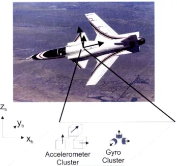
1-2 A complete inertial measurement unit (IMU) includes a cluster of three mu-tually orthogonal accelerometers and three gyroscopes. The body axes of the aircraft are indicated by Xb, Yb, and Zb. ... .. 21

1-3 The computational function of an inertial navigation system integrates IMU measurements (fi) and estimates local gravitational forces (g) to compute an estimate of the current position and velocity (xi(t) and vi(t)). . ... 22 1-4 A simple mechanical accelerometer. ... . . . 24 1-5 A force feedback pendulous accelerometer. . ... 25 1-6 A MEMS accelerometer (left) with a close-up of its structure (right). [Analog

Devices, Inc.] ... .... ... 26

1-7 A microsphere fixed on the end of a fiber stem in a demonstration of a micro-sphere optical resonator accelerometer. Measurement of micromicro-sphere deflec-tions via coupled light into a waveguide may provide pg resolution. [Lai0l] 27 2-1 A 20 ptm glass sphere levitated by a focused laser beam. Photograph taken at

Bell Laboratories in 1971. Adapted from[Ash71] (beam path added for clarity). 30 2-2 Diagram of the reflective and gradient forces on a dielectric sphere. ... 32 2-3 A ray optics diagram of a dielectric sphere in the presence of a laser beam.

The curve below the sphere represents the power distribution in the laser beam. 33 2-4 Light force scaling factors

Q,,

Q

2-5 Plot of the scaling of photophoretic force as a function of the Knudsen number, K n (_ l/p) . . . . 36 2-6 Basic ray optics (left) and exact field modeling (right) show higher intensity

and absorption on the far side of a sphere, indicating that photophoretic forces opposing radiation pressure should occur. ... . . . 37 2-7 Whispering gallery modes (WGMs) are excited by coupling light via internal

reflection into the circumference of a spherical particle. Adapted from [AHV03]. 38 3-1 Diagram of a stable two-beam trap with which optical force rebalancing is

realized. The dashed lines represent gradient forces from both beams. .... 40 3-2 A ray optics diagram of reflected light that forms a spot for particle position

measurement on a split photodetector. ... . . . .. . . 41

3-3 Diagram of the LFA optical rebalancing loop. The acceleration readout of the sensor is the measured difference between the power signals PA and PB on detectors PDA and PDB. ... 41 3-4 Optical rebalancing for zero input (left) and a force F along the beam axis

(right) . . . . 42 3-5 Theoretical precision of a LFA with a particle trapped at the beam waist. For

comparison, experimental results from a demonstrated cold atom gravimeter

are plotted. Adapted from [Sto05]. ... 44

3-6 Diagram of continuous scale factor recalibration concept. . ... . . 45 4-1 Diagram of the experimental apparatus used to demonstrate the feasibility of

a LFA . . . . 50 4-2 Scanning electron microscope image of 1.5 pm fused silica microspheres.

[Cor-puscular, Inc.] . . . ... . . 54 4-3 Picture of vacuum chamber from above. The slide is visible (outlined) with

a distribution of particles on it. The laser beam is directed through the slide

and out of the page. ... 55

4-4 Design of the vacuum chamber that houses the particle launching slide and provides optical access for the levitating beam and detectors. . ... 57

4-5 Diagram of the vacuum system. A turbopump is used for roughing and a getter pump is used for pumping down to high vacuum. . ... 57 4-6 Diagram of the particle position detector. ... . 59 4-7 Diagram of the digital control loop and the source of the error signal e(t). .. 60 4-8 Input-output attenuation of a laser beam by a MEMS FVOA (made by DiCon

FiberOptics, Inc.). ... ... ... ... 60

5-1 A 10 pm borosilicate glass particle (circled on right) levitated by a 75 mW laser beam in the vacuum chamber. Image on the left shows chamber before particle was launched for comparison. Notice how the levitated particle illuminates the chamber with scattered light. ... . 65

5-2 Step response of a levitated particle when optical rebalancing is active and a bias is applied to the feedback loop error signal. . ... 69 5-3 Response of the particle to a step change in bias on the split photodetector

error signal. ... ... 70

5-4 Accelerometer output under constant 1 g input. The short term sensitivity was calculated to be 119 ipg/Hz1/2 . . _. . . . . . . ._. . . ₇₁ 5-5 Discrete Fourier transform of the accelerometer output minus a 1 g offset. .. 72 5-6 Diagram of position resolution experiment. . ... 73 5-7 Top: The split photodetector normalized difference signal measuring

parti-cle oscillations from a sinusoidal power input at 10 Hz (the signal can be calibrated to particle position by the factor 80 /pV/1pm). Bottom: Discrete

Fourier transform of the particle position signal with a peak at the oscillation

frequency f ... ... ... 74

5-8 Example of measured particle shifts which are due to particle surface

irregu-larities ... ... .. 76

5-9 Accelerometer output over a 2.2 hour period. The trend in the top plot can be accounted for by photophoretic forces. ... . 77 5-10 Method for computing the Allan deviation of a time-domain signal. Adapted

5-11 Allan deviations of LFA output for constant 1 g acceleration. The dashed line corresponds to a decrease in bias as 7-1/2

. . . . . . . . . . . . 79

6-1 Diagram of a two-beam LFA using fiber focusers, the existing vacuum chamber

and particle launching slide. ... 83

6-2 Diagram of an alternative particle position detection method involving an

illuminating beam. ... 84

A-I Scattering of a ray by a spherical dielectric particle. . ... 88 B-I Front panel of the particle position control program ... 90 B-2 Diagram of the particle position control program. Elements of the central

stacked structure that are not shown simply calculate the proportional, inte-gral, and derivate control components before being summed in the final frame. 91

List of Tables

1.1 Performance characteristics of several accelerometer types. The silicon

oscil-lating accelerometer is one of the highest performance MEMS accelerometers

to date. [TiWO4], [BaS01] ... ... ... 26

4.1 Characteristics of microspheres used in experiments. . ... 54 4.2 Specifications of MEMS and solid state FVOAs used in experiments .... 61

Chapter 1

Introduction

1.1

Inertial navigation

Inertial navigation is a precise, instrumented method of 'dead reckoning,' in which accelera-tion in inertial space is sensed as an applied force on a physical body, and used to calculate the current position and velocity, or state. With a well-known initial state, the effects of these external forces on the body's motion may be continuously evolved without making external references to the vehicle's position, thus providing an 'onboard' method for navigation.

Inertial navigation systems, therefore, provide a determination of vehicle position and velocity in a chosen inertial reference frame without the need for external measurements, which all other navigation methods require. A system of onboard sensors and data processors perform navigation functions continuously by incorporating force measurements into models of vehicle dynamics and producing an estimate of current position and velocity. Given estimates of the initial state and subsequent measurements of acceleration and orientation, kinematic equations describing the motion of a body in inertial space may be integrated to compute the current state. Independent, onboard operation with automated computational tasks is the essential advantage of inertial navigation systems, since external measurements needed for other navigation systems may be intermittent, compromised, or inaccessible.

To determine position and velocity, an inertial navigation system must perform three functions. First, it must be able to refer inertial measurements to an inertial reference frame. This involves both a mechanization of inertial coordinates (e.g., geocentric longitude,

latitude, and altitude) relative to a body's physical coordinates (e.g., an aircraft's body axes shown in figure 1-2) and a computational relation between the body axes and other relevant coordinate frames. For instance, a satellite's body coordinates must be related to geocentric coordinates for navigation in orbit. The second function an inertial navigation

x(O)

S.

x(t)

Sz,

.(t)

_z

Figure 1-1: Principle of deduced, or 'dead' reckoning. If the original state [£(0), (0)] is known and the system's orientation and acceleration over time are known, the state at time t can be completely reconstructed.

system performs is the measurement of specific force, or the change of a body's momen-tum relative to inertial space'. This is accomplished with accelerometers, sensors which measure specific force along sensitive axes. As shown in figure 1-2, an ensemble of three orthogonally-oriented accelerometers is implemented to measure inertial acceleration in all three dimensions. These accelerometers may be installed on a gyroscopically stabilized plat-form so that the accelerometers' axes are fixed relative to inertial space (platplat-form system), or 'strapped' down to the body frame (strapdown system). In the latter case gyroscopes, which measure angular velocity, sense changes in body heading relative to inertial coordi-nates. A complete system of accelerometers and gyroscopes, as shown in figure 1-2, is called an inertial measurement unit (IMU).

The final function of an inertial navigation system is the integration of specific force measurements from accelerometers to determine velocity and position. Figure 1-3 shows a diagram of this computation. Numerically integrating Newton's kinematic equations in

'Specific force is measured as the difference between the body's acceleration in inertial space and the local gravitational force. Accelerometers measure specific force, not inertial acceleration.

Lb

4 I

Yb

Accelerometer Gyro Cluster Cluster

Figure 1-2: A complete inertial measurement unit (IMU) includes a cluster of three mutually orthogonal accelerometers and three gyroscopes. The body axes of the aircraft are indicated by Xb, Yb, and Zb.

three dimensions provides estimates of velocity and position. It should be noted that, due to the equivalence principle, it is impossible to distinguish gravitational forces from iner-tial accelerations (e.g., rocket thrust or vibrations) with accelerometer measurements alone. Models of local gravitational fields are required to calculate the gravitational component of the measured force. The equation to calculate inertial acceleration, i., from accelerometer measurements is:

r Ca + G (1.1)

where fa is the specific force vector along accelerometer axes, Ca is a rotational

transforma-tion from accelerometer axes to inertial coordinates, and Gi is the computed acceleration

due to gravity.

High precision sensors are essential for inertial navigation systems, since errors in ac-celerometer measurements lead to position errors which grow as the square of time (the result of integrating these measurements twice with respect to time). For instance, a con-stant accelerometer bias 6a, or measured offset from the true acceleration, contributes to a

Navigation Computer

IMU

Accelerometers:

oOrsco.pes,,

,

tzb

_{i I}

_b

Figure 1-3: The computational function of an inertial navigation system integrates IMU measurements (fi) and estimates local gravitational forces (gi) to compute an estimate of the current position and velocity (x (t) and vi(t)).

position error 6r in one dimension of

6r = v₀ot + -(a)t 2 _(1.2)

2

where vo is the initial velocity. Therefore, a bias of 0.1 mg measured over one hour results in a position error of over 6 km (with vo = 0). While external measurements like radar position updates can reduce the growth of these errors, systems operating in environments without access to these references (e.g., long duration space flight) must rely on inertial navigation for long periods of time. These applications place a premium on the precision of inertial sensors.

1.1.1

History and applications

While gyroscopic measurements of the Earth's rotation were made as early as the 1850s, navigation applications of inertial sensing were not pursued until shortly before World War II, when German rocketry pioneers developed the V-2 with a complete gyro-stabilized IMU for trajectory control [Mac90], [Bar01]. In fact, guided missile and rocketry programs such as the U.S. Navy's Fleet Ballistic Missile program are responsible for driving much of the innovation in inertial guidance systems, both in improving the performance of inertial sensors and in revolutionizing the power and size of computers [Mac90].

iI II_I I I I II I II I I I II I I I_I II II I

In the 1960s, Charles Stark Draper headed the development of an IMU at the MIT Instrumentation Laboratory for spacecraft guidance and navigation as part of NASA's Apollo Program. Each flight to the Moon demonstrated that an inertial navigation system with updates from astronaut star-sightings (which soon became automated with star tracking cameras) could provide sufficient navigation accuracy for three-day spaceflights. Since the Apollo era, deep space missions such as the twin Voyager probes have used continuously operating inertial navigation systems for over thirty years. Similarly, submarines require high performance inertial navigation systems for underwater navigation over periods as long as several months.

Now that the need for precise inertial instruments has been motivated, a brief introduction to the principles of accelerometers is in order2_{. These concepts will help frame the discussion}

of the accelerometer which is the subject of this thesis.

1.2

Principles of accelerometers

Accelerometers measure the inertial force on a mass when it accelerates with respect to inertial space. A simple accelerometer, shown in figure 1-4 , includes a mass called the 'proof mass' which is connected to a case or platform by springs. If a force F is applied to the case, the proof mass will resist the force against the springs because of its inertia. As a result, the mass will be deflected with respect to the case. This displacement is proportionally related to the force applied to the case, so measurement of the proof mass displacement (made by a 'pick-off' device) provides a measure of F.

In the presence of gravitational forces, however, the case and proof mass accelerate to-gether. Accelerometers are therefore not sensitive to gravitational acceleration. This fact is the underlying reason for requiring gravity models in inertial navigation systems to navigate in the presence of a gravitational field. An accelerometer measures specific force, or the non-gravitational force per unit mass.

2_{As gyroscopes are not the subject of this thesis, the fundamentals of their operation are not described}

here. Comprehensive descriptions of gyroscopic measurement and currently used gyroscopes can be found in [Law98] and [TiW04].

External force (F

Case

Proof mass

Exeralfoce(FUW

AVIVVvI

I

I

Displacement

pick-off Signal proportional to specific force

Figure 1-4: A simple mechanical accelerometer.

1.2.1

Force feedback accelerometers

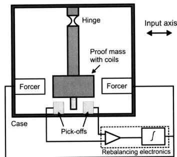
The simple instrument shown in figure 1-4 may be described as an 'open loop' accelerometer, in that the measurement of specific force is made by passively tracking the deflections of the proof mass. An alternative approach to measuring specific force involves the use of actuators to 'null' or cancel proof mass motion from a 'zero' position, or set point. Figure 1-5 shows a basic force feedback accelerometer in which the deflections of a magnetic proof mass from the set point are nulled by electromagnetic forcers (magnetic coils). These forcers are controlled by a feedback controller known as a force rebalancing loop. The measurement of specific force is then made by monitoring the current applied to the forcers for rebalancing, as opposed to the measurement of proof mass motion.

Force feedback accelerometers are typically more precise because it is in general easier to measure a set point than a range of displacements. For systems measuring high acceleration, open loop accelerometers are typically limited by nonlinearities in the displacement per unit force (e.g., when spring extension is no longer linear). As a result, most high precision or high input accelerometers use force feedback.

1.3

Current accelerometers

Accelerometers are used in inertial navigation systems, as already discussed, but they serve a host of other applications as well. Some of these applications include equipment stabilization

Figure 1-5: A force feedback pendulous accelerometer.

and control (e.g., active automobile suspension), gravimetry, and even entertainment (e.g., the Nintendo Wii controller). These applications demand a broad range of performance, size and cost requirements, and have influenced the development of several different classes of accelerometers. Mechanical accelerometers still achieve the highest performance overall, but microelectromechanical systems (MEMS) sensors are gaining prominence for their lower cost, batch manufacturability, low power usage, and reasonable performance (see figure 1-6). Table 1.3 summarizes typical performance parameters for several current sensors types.

The most commonly reported parameters are bias stability, scale factor stability, and resolution or sensitivity. Bias is a nonzero offset measured for zero acceleration input, and can change over time (hence, bias stability). Scale factor is the ratio of accelerometer output (e.g., an electrical current) to acceleration input. Scale factor can also change over time (hence, scale factor stability), leading to errors whenever there is a nonzero acceleration. Typically, the fractional variation over time is quoted in units of parts per million (ppm). Finally, resolution and sensitivity measure the lower limit in input below which acceleration measurement is masked by noise (usually quoted in g for resolution or g/Hz1/2 for sensitivity, since the measurement error due to white noise should decrease as the square root of the measurement interval).

Accelerometer Type _{Mech. pendulous MEMS pendulous Silicon oscillating}

Maximum input (g) 100 50 120

Scale factor stability (ppm) 100 500 5

Bias stability (Pug) _{0.1-10 100-1000 5}

Resolution (pg) 10 1000 10

Table 1.1: Performance characteristics of several accelerometer types. The silicon oscillating accelerometer is one of the highest performance MEMS accelerometers to date. [TiW04], [BaSO1]

Figure 1-6: A MEMS accelerometer (left) with a close-up of its structure (right). [Analog Devices, Inc.]

1.3.1

Optical accelerometers

Rapid advances in commercially available compact laser systems, fiber optics, and electro-optic components have generated interest in developing high precision optical inertial sensors. Optical gyroscopes, such as the ring laser gyroscope and fiber optic gyroscope, are already being used for high-accuracy inertial navigation. Fewer optical accelerometers have been developed, but this class of sensors promises high performance, particularly in sensitivity and resolution. The fiber optic accelerometer, which measures phase shifts in an interferometer

due to deflections of an optical fiber, has achieved a resolution of 1 pg [Tve80]. More recent optical accelerometer concepts, such as a microsphere optical resonator accelerometer (shown in figure 1-7) and the light force accelerometer presented in this thesis, may ultimately achieve sensitivities in the range of ng/Hzl/2 in simple, compact systems.

Fiber Stem Microsphere

Z

/

N N

Epoxy Bead Waveguide Chip

Figure 1-7: A microsphere fixed on the end of a fiber stem in a demonstration of a microsphere optical resonator accelerometer. Measurement of microsphere deflections via coupled light into a waveguide may provide pg resolution. [Lai0l]

The light force accelerometer studied in this thesis is essentially an optical force rebalanc-ing accelerometer; instead of usrebalanc-ing magnets to rebalance proof mass motion, it uses radiation pressure, or the momentum transfer from light to a reflecting object, provided by high power laser beams. The proof mass is a glass microsphere, which is levitated and trapped by two laser beams. In fact, the measurement of proof mass displacement and acceleration are both made by optical detection, allowing for high precision. This thesis takes a first step in demonstrating this interesting concept.

1.4

Overview of Thesis

This thesis covers the development of the light force accelerometer (LFA) concept to an experimental demonstration of the concept's major components, including laser levitation of glass microspheres in high vacuum and optical force rebalancing. The results of this work suggest future steps for realizing a complete LFA, and discuss elements of the accelerometer which will affect its performance. In Chapter 2, the mechanics of particle trapping with a laser beam are discussed as an introduction to the LFA concept. Several optical effects which affect performance are also presented. Chapter 3 develops the concept of optical force rebalancing and its use in the LFA, and outlines its major advantages and limitations. Chapter 4 describes the experimental apparatus used to demonstrate the feasibility of the LFA and obtain preliminary performance diagnostics. Descriptions of laser sources and important electro-optic components are included. The results of demonstrations of particle trapping in high vacuum and optical force rebalancing are covered in chapter 5. Preliminary performance diagnostics for a constant 1 g acceleration, including short term sensitivity and bias stability, are also presented. Chapter 6 concludes the thesis by proposing future steps for realizing a complete LFA and testing its ultimate performance.

Chapter 2

Optical Trapping

2.1

Origins of Optical Trapping

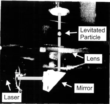
With the invention of the laser in the early 1960s, high intensity and high gradient light sources became easily attainable in a laboratory. Later in the decade, physicist Dr. Arthur Ashkin of Bell Laboratories calculated that a laser beam focused onto a microscopic particle could exert a large force through radiation pressure, or the transfer of momentum from light to a reflecting surface [Ash97]. Soon after, Ashkin experimentally demonstrated that laser light would not only push small latex spheres in a fluid, but could also confine them within the beam. A combination of two counter-propagating laser beams created the first three-dimensional optical trap with a micron-sized latex microsphere suspended in water [Ash70]. In 1971, Ashkin levitated a 20 pm glass sphere in air (against gravity) with a single vertical laser beam (shown in figure 2-1), and reported stable trapping for many hours [Ash71].

The achievements of these experiments availed a new method for the clean and precise manipulation of microscopic particles. Extensions of these techniques have made a significant impact in other fields, including biology and atomic physics [Chu85], [RaP87]. The use of 'optical tweezers,' as this method is called in biology, have made studies of microscopic biological systems like RNA-DNA transcription and the fusing of cells possible [Fin94]. In physics, the trapping of neutral particles led to the discovery of atom trapping techniques, known as laser cooling, and major advancements in high precision atomic spectroscopy and atom interferometry [Kas89], [DaK95].

Figure 2-1: A 20 ym glass sphere levitated by a focused laser beam. Photograph taken at Bell Laboratories in 1971. Adapted from[Ash71] (beam path added for clarity).

2.1.1

_{Application to inertial sensing}

One of the important later achievements in the optical levitation of glass particles was trap-ping in high vacuum, where viscous drag and other thermal effects are negligible [Ash76]. Ashkin reported that, "If the viscous damping [of air] can be further reduced, applications to inertial devices such as gyroscopes and accelerometers become possible" [Ash71]. No sensor development was pursued for such an application, however, because of the state of laser and vacuum technology at the time. Subsequent advancements in both fields, however, renewed interest in precise sensors using levitated dielectric particles. The light force accelerometer (LFA), which uses a levitated microsphere as a proof mass, is an example of such an instru-ment. Before presenting the LFA concept, however, a description of the optical trapping of neutral particles is in order.

2.2

_{Mechanics of optical trapping}

The system of interest for optical trapping is a spherical dielectric particle placed in a Gaussian-like laser beam. A basic ray optics model of light reflection and transmission

through the sphere illustrates how the laser beam confines the sphere within the beam and accelerates it in the beam direction'. By breaking up a laser beam into individual rays and modeling their reflection, refraction, and transmission at the surface of a particle, one can determine the transfers of momentum from light to the particle.

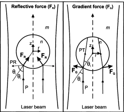
Consider a dielectric sphere with index of refraction n in a gas with index m, and that n > m (otherwise, particles will be forced out of the beam rather than trapped). Figure 2-2 diagrams the forces exerted to a sphere when a ray of power P meets the surface of a dielectric sphere at an angle Oi from the normal. The first force is due to reflection (also known as radiation pressure)2. A component of the ray is reflected with power PR, where R is the Fresnel reflection coefficient (assuming the ray is unpolarized):

1 2 sinJ 2 t a t

R = -(Rs + Rp) = (sin(t i) + (tan(t - i) (2.1)

2 2 sin(Ot + i) tan(0t + Oi)))

Rs and Rp are the reflection coefficients for polarization components in and out of the plane of incidence and Ot is the angle of the transmitted ray relative to the normal (defined by Snell's law). The incident ray has a momentum of m per second, and upon reflection a

component of this momentum is imparted to the sphere. The magnitude of the force is dependent on the incident angle O, and is a maximum of 2_mP - _{for a complete retro-reflection}

(when Oi = 0). Since the sphere is in the center of the beam, a symmetrically situated ray exerts a force of the same magnitude. The radial components, however, cancel out and the net force points along the direction of the beam (+z); thus, the reflective force accelerates a particle along the beam axis.

Another portion of the ray is transmitted with power PT, where T is the Fresnel trans-mission coefficient (T = R - 1). As the right side of figure 2-2 shows, the transmitted ray is refracted and deflected toward the center of the beam. To conserve momentum, a force is exerted on the sphere away from the beam axis (-r). A symmetric ray cancels out this 'It should be noted that the ray optics model presented here is accurate for particles which are much larger than the wavelength of the light. As will be seen, this assumption is appropriate for microspheres used in the light force accelerometer. For particles which are small compared to the wavelength, however, this description breaks down. Rayleigh particles, as they are known in the literature, act like basic dipoles and cannot be treated with a simple ray picture.

2In the literature, this force is commonly called the scattering force, since for more sophisticated analysis the light is scattered by dipole radiation. 'Reflective' force is chosen here since it is appropriate for the

I

\

*

I m

I

Laser beam

Figure 2-2: Diagram of the reflective and gradient forces on a dielectric sphere.

radial force, as shown in the diagram. This force will be referred to as the gradient force, since it is produced by the focusing of the beam through the sphere3.

To demonstrate how these forces can trap a spherical particle in a laser beam, consider the case when the particle is radially displaced from the axis of the beam. Figure 2-3 shows the reflective and gradient forces from rays symmetrically situated about the particle. As was just shown, the net reflective force due to each ray (Fi and FR2) is in the direction of the laser beam. The radial components for the input and output rays roughly cancel out (e.g., Fk, cancels out FRl in the radial direction); the sum of the gradient forces, however, produces a net radial force. While the force vectors for the rays 1 and 2 are radially symmetric, beam

1 contains significantly more power (it is closer to the center of the beam). Therefore,

FG1 > FG2 and the net force points in the -r direction (see the sum of forces diagram in figure 2-3). If the particle were displaced to the other side of the beam, the net gradient force would also point toward the center of the beam. It is now clear that a laser beam

3In the literature, this force is also referred to as the gradient force. The reason is clear when looking at the definition of this force on a Rayleigh particle, which is treated as a simple dipole: FG -- lmVE2,

where a is the polarizability of the particle, m is the particle mass, and E is the electromagnetic field of the light. The 'trapping' potential due to this force is simply UG = amE2, so it is clear that a higher intensity

beam (I - E2) creates a deeper potential and stronger trap.

1

I

P

i

accelerates the particle along the beam axis and transversely traps it. Ray Reflected ray Force N (I) X

E

m

Ir

Sum of forces (F,o,)

-r

Figure 2-3: A ray optics diagram of a dielectric sphere in the presence of a laser beam. The curve below the sphere represents the power distribution in the laser beam.

To calculate the total force a ray exerts on a sphere, the reflective and gradient forces due to each reflection and transmission at the surface of the sphere must be summed. In general, a convenient representation of the net force components in the radial (r) and axial (z) is mP Fr Q=r (2.2) and mP

Fz = Qz

P

where Q, and Qz are dimensionless factors dependent on 0i and the relative index of the sphere and surrounding gas, n/m. Fr is roughly equal to the reflective force and Fz is roughly equal to the gradient force (it will be shown that it is more convenient to calculate the forces

-o

I*-#-1

along the axes). The total force on a particle exerted by a ray, therefore, is

F =mP Q mP

F = Q-

= /Q +

There are several methods for calculating Q, but the simplest is to sum up the force contri-butions for an infinite series of internal reflections and transmissions (see figure A-1). This derivation is somewhat tedious, and can be read in detail in appendix A.

It is interesting to consider the relative magnitudes of the reflective and gradient forces. Figure 2-4 shows each

Q

Figure 2-4: Light force scaling factors Qr, Qz, and Q as a function of Oi, with a relative index of n/m = 1.45.

The discussion of optical forces in this section can account for the behavior of a dielectric sphere trapped in a laser beam when the surrounding gas is at atmospheric pressure or high vacuum. In between these pressure regimes, however, other thermal effects related to the absorption of light in the sphere, known as photophoretic effects, contribute significantly to the dynamics of the trapped sphere.

2.3

Photophoretic Effects

The absorption of light by a particle results in heating of the particle and the surrounding gas. When this heating occurs non-uniformly, the gas exerts a force on the particle4_{. For a}

spherical particle in a laser beam, it is possible for heating to be dominant on the incident or far side. The photophoretic force then points along the beam axis and either adds to radiation pressure ('positive' photophoresis) or opposes it ('negative' photophoresis) [Plu85]. Furthermore, the overall magnitude of the force is strongly pressure dependent. In the limit of high vacuum, of course, there is no photophoretic force. This section serves to provide an understanding of these effects, since these forces contribute to significant biases in the LFA. The theory of aerosol mechanics has developed a basic description for the photophoretic force on a spherical particle in a laser beam. The force is represented as

FR = - 4 7J (2.5)

pgTsKi

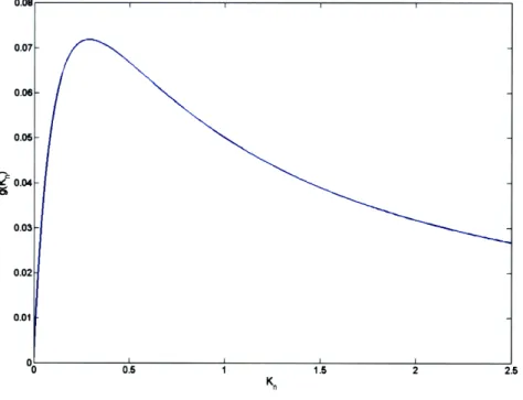
where R is the particle radius, 7le is the gas viscosity, K is the coefficient of thermal slip (- 1), Ts is the surface temperature, p, is the density of the external gas, Ki is the internal thermal conductivity, and I is the intensity on the particle [Yal76]. The most important factor in the equation, however, is the dimensionless factor J. J measures the non-uniformity of the intensity distribution within the particle, and is proportional to the absorption efficiency of the particle material (capturing the spectral properties of the effect). Ultimately, this factor determines whether negative or positive photophoresis occurs.

The formula in equation 2.5 is only accurate in the regime where the mean free path of the surrounding gas is much smaller than the particle size (e.g., atmospheric pressure), but the model can be extended to low and high pressure by a scaling law

1 1

g(Kn) = 1 + 3CmKn 1 + 2CtKn (2.6)

where K, is the Knudsen number, or the ratio of mean free path to the particle size (propor-tional to l/p, where p is the pressure) and Cm and Ct are empirically determined coefficients

4

Photophoretic effects apply in much larger systems as well. These forces are thought to be the source of particle depletion around stellar bodies [WuK05], and are potentially strong enough to 'levitate' particles

(typically Cm ~ 1 and Ct - 2) [Ree77]. The pressure-dependence of photophoretic force is plotted for a range of K in figure 2-5. Clearly, this effect peaks when the mean free path is comparable to the particle size (K, , 1). In this critical pressure regime, a particle may be destabilized and ejected from a laser beam. Thus, photophoretic forces may generate bias and stability problems in the light force accelerometer.

2r

Figure 2-5: Plot of the scaling of photophoretic force as a function of the Knudsen number,

Kn

(~

A spherical particle in a laser beam will focus light, leading to higher absorption on the far side of the particle (as shown on the left in figure 2-6). This indicates that gas heating on the far side will lead to negative photophoresis. Exact modeling of the intensity distribution inside a 10 1m sphere (shown on the right in figure 2-6) verifies that absorption and therefore

heating are greatest on the far side of the particle5_{. As will be discussed in the results of}

this work, experiments with glass microspheres trapped in a laser beam observed significant negative photophoresis. While beam shaping or selection of larger or smaller particles may

5

This plot was produced by a simulation of electric field distribution in a homogeneous sphere, using a rigorous derivation from classical Mie theory. Mie theory solves the problem of a plane wave scattered by a homogeneous sphere, and provides exact solutions of the internal and external fields. While the derivation and presentation of these results is beyond the scope of this chapter, they can be found in several sources [VDH81] (Chapter 9), [BAS88], [BAS89].

influence the magnitude of photophoretic a low absorption material like fused silica

effects, the simplest way to reduce glass. them is to use

Ray optics

SI

Laser beam

I

ILaser

beam

+

Figure 2-6: Basic ray optics (left) and exact field modeling (right) show higher intensity and absorption on the far side of a sphere, indicating that photophoretic forces opposing radiation pressure should occur.

2.3.1

Other significant optical effects

Finally, a few optical effects which could influence trapped particle behavior are included for reference in later chapters. The discussion of optical effects thus far has not addressed another result of absorption in a particle. When circularly polarized light is absorbed in a particle, a torque is exerted on it. The classical interpretation is that angular momentum in an electromagnetic wave is absorbed and transferred to the particle as mechanical angular momentum. The quantum mechanical picture describes photons as having 'spin' angular momentum in integer amounts of uzh (a, =

+1),

1= Pabs

W - " (2.7)

where w is the frequency of the laser and Pabs is the absorbed power [Fri96]. The absorbed power is a function of the optical power and the absorption coefficient, which is about

Field modeling

t

,-|

1

k

1

10-5cm- 1

for 1 pm light in fused silica glass. If rotation of a particle is undesired, then linear polarization must be maintained. In principle, a trapped particle in vacuum may continue to accelerate to extremely high frequency, since there would be no viscous drag [Ash74]. For irregularly shaped particles, rotations may lead to instability and ejection from the laser beam.

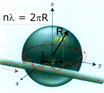
The last optical effect considered here involves internal optical resonances known as 'whispering gallery modes' (WGMs), which could alter the force of light on a spherical particle when excited. In a glass sphere, light may couple into internal modes when the circumference of the sphere is equal to an integer numbers of wavelengths. In a micron-sized sphere, these resonances are very sharp and may achieve quality factors as high as 109. WGMs, therefore, may provide a tool for precise measurements of particle size if a mode can be locked to with the laser frequency. However, if the frequency of a freely running laser drifts across a WGM resonance, the power coupled into the sphere is suddenly increased. As a result, the optical trapping forces exerted by the laser beam would change. In the light force accelerometer, this would generate large biases. The next chapter will address this and other potential limitations in the accelerometer concept.

z

=nk

2nRI

Figure 2-7: Whispering gallery modes (WGMs) are excited by coupling light via internal reflection into the circumference of a spherical particle. Adapted from [AHV03].

Chapter 3

Light Force Accelerometer Concept

This chapter presents the principles of the light force accelerometer (LFA) concept and discusses some of its notable advantages and limitations. The discussion focuses on the essential functions of the accelerometer, and how a high sensitivity sensor could be built from them.

The LFA concept was motivated by demonstrations of the optical levitation of glass microspheres, and the proposal by Arthur Ashkin that precise inertial sensors could be made from a system using a levitated dielectric particle as a proof mass [Ash71], [Ash77]. While the pursuit of such a sensor was limited by the state of laser and vacuum technology, rapid advancements in compact, high power laser sources and electro-optic technology during the last 30 years has made it feasible to develop a compact LFA [Kel05].

3.1

Optical force rebalancing

The LFA measures acceleration through optical force rebalancing, or the rebalancing of inertial forces on a levitated proof mass by radiation pressure from a laser beam. As discussed in chapter 2, a laser beam both accelerates a dielectric sphere along its axis (radiation pressure, or reflective force) and transversely confines it within the beam (gradient force). A stable trap can be created, as was done in Ashkin's work, by placing a glass microsphere in a vertical laser beam with sufficient power for radiation pressure to balance gravity. Without the presence of gravitational forces, a trap can be formed by placing a sphere within two counter-propagating beams, as shown in figure 3-1. This configuration allows for a single-axis

accelerometer to operate in any orientation.

Input axis

4

F

I

I

Figure 3-1: Diagram of a stable two-beam trap with which optical force rebalancing is realized. The dashed lines represent gradient forces from both beams.

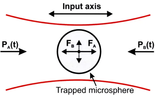
To enable rebalancing, the proof mass position must be measured along the beam axis (also the input axis). Interestingly, this can be accomplished with the light reflected off the proof mass. Figure 3-2 shows how light is reflected perpendicularly to the laser beam from a levitated sphere'. This reflected image is then focused onto a split photodetector, as shown in a diagram of the rebalancing loop (figure 3-3). The detector provides the reference position, or set point, for rebalancing. The normalized difference signal from the detector (difference between the upper and lower signal divided by their sum, A/E in figure 3-3) is proportional to particle displacement, and is used to maintain the particle position by adjusting the beam powers with variable optical attenuators (VOA).

If there is no net force on the sensor, equal powers in beams A and B will maintain the particle position (left, figure 3-4). When a force F is applied to the sensor, the proof mass position is maintained by proportionally increasing the power in beam A (right, figure 3-4). Equilibrium is reached when the difference in the reflective force of the beams balances F (i.e., FA - FB = _{F). Since the magnitude of the reflective forces is proportional to the}

power of a laser beam, acceleration may be calculated from the power difference of the

1

The reflection from the bottom surface of the particle and the transmission from the top surface actually create two spots (a and b in figure 3-2). For small particles, however, these two spots are difficult to resolve because they are spaced approximately one particle diameter apart.

Laser beam

Figure 3-2: A ray optics diagram of reflected light that forms a spot for particle position measurement on a split photodetector.

ration

lout

Figure 3-3: Diagram of the LFA optical rebalancing loop. The acceleration readout of the sensor is the measured difference between the power signals PA and PB on detectors PDA and PDB.

beams(PA(t) - _{PB(t)). The accelerometer readout, or the output signal of the sensor, is} measured as the difference between the photodetector signals PDA and PDB, as indicated in figure 3-3.2

No force

Platform

_Platform

Figure 3-4:

(right). Optical rebalancing for zero input (left) and a force F along the beam axis

3.2

_{Advantages of the LFA}

The expected performance of the LFA will now be addressed. Several salient features of the LFA concept make it capable of high sensitivity and scale factor stability. These advan-tages arise from the noise statistics of the acceleration measurement and the potential for continuous recalibration in a device. A brief description of these factors is included below.

3.2.1

Accelerometer noise statistics

Optical force rebalancing provides a low noise acceleration measurement when a levitated sphere is trapped in high vacuum. Considering a simple case where a glass sphere is levitated by a single laser beam against a constant 1 g acceleration, the fractional noise in a

measure-2

Note that portions of the light going to the proof mass in beams A and B are measured (the measurement beams), rather than the actual powers incident on the particle. Still, the measured power difference is proportional to F. PA

PB

-Split

PD

4

PB

tr

€

ment of g is equal to the fractional noise in measurement of the steady-state levitating beam power Po:

g (t) _-=- JP(t)

(3.1)

g Po

where 6g(t) is the RMS value of the acceleration measurement and 6P(t) is the RMS value of the measured optical power. While a detailed noise statistics analysis is beyond the scope of this chapter, a simple model of noise processes including laser relative intensity noise and shot noise for the measurement of the levitating beam power shows that the laser noise integrates down as 1/(measurement interval) to the shot noise limit [Sto05]. Figure 3-5 plots the expected acceleration error for this single-beam LFA when the proof mass is levitated in high vacuum (where Brownian noise and photophoretic forces are eliminated). Neglecting other noise processes, the LFA was estimated to attain under 10 ng of measurement error in only 10 seconds of averaging, which is a precision comparable to a demonstrated cold atom gravimeter [PeC01]. While a real system will probably not achieve this ideal performance, the LFA is a considerably simpler system and is much easier to shrink to a compact sensor than a cold atom instrument.

3.2.2

Scale factor linearity

Like other force feedback or rebalancing accelerometers, the LFA should achieve a linear scale factor over a large range of acceleration (dynamic range). The dynamic range of the LFA depends primarily on the total power available for rebalancing, which is proportional to the maximum reflective force that one of the laser beams could exert on the levitated proof mass. The scale factor of the LFA is the ratio of the optical power required for rebalancing per unit acceleration. Nonlinearities in scale factor arise when the proof mass heats and expands from absorption. Scale factor will decrease as a particle expands, since it will reflect more light and thereby require less optical power to rebalance. This nonlinearity may be avoided in practice by maintaining the total power in both beams so that the total absorption does not change (rebalancing would simply redistribute the power between the beams).

Another source of scale factor nonlinearity is the coupling of light into whispering gallery modes (see section 2.3.1 for a basic discussion of these resonances). This effect is negligible for small spheres (5-20 pm range), but is potentially significant for particles greater than

1 L_

0

E

0.1

1

10

100

1000

Measurement interval (s)

Figure 3-5: Theoretical precision of a LFA with a particle trapped at the beam waist. For comparison, experimental results from a demonstrated cold atom gravimeter are plotted. Adapted from [Sto05].

^

500 ,pm. Whispering gallery modes in glass microspheres achieve some of the highest quality resonances known (Q - 109, [Ver98]). Excitation of a WGM would decrease the amount of reflected light, requiring more incident power for rebalancing the same inertial acceleration. Fortunately, these effects may be avoided by active laser frequency stabilization or ensuring the laser frequency remains between these broadly separated resonances. For instance, a 10 pm sphere has circumferential whispering gallery modes spaced by 6v = c/(27rD) - 4.7 THz. Since most laser frequencies are stable to a band much smaller than this spacing, a particle would need to nearly double in size before the next resonant mode would be excited (for a thermal coefficient of < 1 ppm/°C in silica glass, this is not possible).

3.2.3

Scale factor stability and continuous recalibration

PO

+ 6Psin(wt)

P, - 6Psin(wt)

6x(w)

Figure 3-6: Diagram of continuous scale factor recalibration concept.

While optical rebalancing should provide a linear scale factor over a large dynamic range, it does not necessarily guarantee long term stability. Scale factor drifts may occur because of long term drifts in electronics (e.g., amplifier gain drifts). These drifts can be measured and used to calibrate acceleration measurements continuously with the following technique. Calibration is achieved by dithering both levitating beam powers at frequency w, as shown in figure 3-6). The proof mass will oscillate in response. With continuous measurements of its average oscillation amplitude, 6x(w), and the fractional power amplitude, 6P, the scale factor may be updated (the frequency of the dither, w, would be made faster than vehicle dynamics and the accelerometer bandwidth). Quantitatively, the scale factor is related to

these amplitudes by

SP

K = (3.2)

The proof mass response is represented by a simple second order system nSP

m6i(w, t) = m(6x)w2cos(wt + q) = - cos(wt) (3.3)

where m is the particle mass, 65(t) is the particle acceleration due to the dither, n is the surrounding gas index of refraction, and c is the speed of light. Therefore, the precision of a scale factor measurement ultimately depends on the resolution of particle position and the optical power amplitude (6P). Both of these signals are measured on photodetectors, so the fundamental noise limit is shot noise in each case. The fractional uncertainty in scale factor measurement is

AK A(6x(w) 2 ( ) _(3.4)

6x(w) + P

where AK, A(6x(w)), and A(6P)) are the RMS noise values of the scale factor, position and power dither amplitudes, respectively. Assuming that the each measurement is shot noise-limited, and that the power of the particle image focused on the split photodetector is 15 pW, scale factor resolution is limited to 0.1ppm/VH1 _{z. For continuous recalibration, the}

resolution is equivalent to scale factor stability.

3.2.4

Radiation hardness

While system survivability in the space environment is not an immediate concern in this work, it is worth noting that the optical components of a LFA are intrinsically radiation hard. Most optical components in the system have been extensively tested for previous spaceflight programs, and it is likely that the LFA would serve well as an inertial sensor for spacecraft navigation.

3.3

Concept Limitations

A few potential limitations of the LFA deserve mention before a description of the current apparatus in the next chapter. Several few practical issues present interesting challenges for