Methods and applications of shear wave splitting: The East European Craton

(1)

HAL Id: tel-00539114

https://tel.archives-ouvertes.fr/tel-00539114

Submitted on 24 Nov 2010

Methods and applications of shear wave splitting: The

East European Craton

Andreas Wüestefeld

To cite this version:

Andreas Wüestefeld. Methods and applications of shear wave splitting: The East European Craton. Geophysics [physics.geo-ph]. Université Montpellier 2 Sciences et Techniques du Languedoc, 2007. English. �tel-00539114�

(2)

UNIVERSITE MONTPELLIER II SCIENCES ET TECHNIQUES DU LANGUEDOC

THESE

pour obtenir le grade de

D

OCTEUR DE L

’U

NIVERSITE

M

ONTPELLIER

II

Discipline : Géophysique Interne

Formation Doctorale: Structure et Evolution de la Lithosphère

Ecole Doctorale: Systèmes Intégrés en Biologie, Agronomie, Géosciences, Hydrosciences, Environnement

présentée et soutenue publiquement par

A

NDREAS

W

ÜSTEFELD

le 27 Septembre 2007

TITRE

Methods and applications of shear wave splitting: The East European Craton Methods et applications des ondes des cisaillement : Le Craton de l’Europe de l’Est

JURY Marc DAIGNIERES Götz BOKELMANN Jean-Paul MONTAGNER Paul SILVER Alain VAUCHEZ Martin SCHIMMEL President Directeur de Thèse Rapporteur Rapporteur Examinateur Examinateur

(3)

(4)

T

a

b

l

e

o

f

C

o

n

t

e

n

t

s

:

0. RESUME EN FRANÇAIS ... 1

0.1.SPLITLAB... 4

0.2.CRITERE DE “NULL” ... 5

0.3.BASE DES DONNEES DE « SHEAR WAVE SPLITTING » ... 7

0.4.L'ANISOTROPIE DU CRATON EST EUROPEEN... 7

1. THESIS MOTIVATION ... 11

1.1.THESIS OUTLINE... 13

2. LINEAR ELASTICITY AND WAVE PROPAGATION ... 15

2.1.HOOKE’S LAW... 17

2.2.ISOTROPIC MEDIA... 18

2.3.ANISOTROPIC MEDIA... 20

2.4.PLANE WAVE PROPAGATION... 22

2.5.SEISMOLOGICAL DETECTION OF ANISOTROPY... 25

2.5.1. P-waves ... 25

2.5.2. Shear wave splitting ... 25

2.5.3. Surface waves... 28

3. ORIGINS OF SEISMIC ANISOTROPY... 29

3.1.LATTICE-PREFERRED ORIENTATION (CRYSTALLINE ANISOTROPY)... 30

3.2.SHAPE-PREFERRED ORIENTATION (ALIGNMENT OF STRUCTURES) ... 31

3.3.DEPTH OF ANISOTROPY... 32

3.3.1. Anisotropy in the crust ... 33

3.3.2. Anisotropy in the lithosphere ... 34

3.3.3. Anisotropy in the asthenosphere ... 34

3.3.4. Anisotropy in the transition zone... 36

3.3.5. Anisotropy in the lower mantle ... 36

3.4.SEISMIC ANISOTROPY AND PLATE TECTONICS... 37

3.4.1. Rifting... 37

3.4.2. Subduction... 39

3.4.3. Orogens... 40

(5)

4.1.OVERVIEW... 43

4.2.INVERSION TECHNIQUES... 45

4.3.SPLITLAB:A SHEAR-WAVE SPLITTING ENVIRONMENT IN MATLAB... 48

4.3.1. Abstract ... 48

4.3.2. Introduction... 48

4.3.3. Modules Description ... 51

4.3.3.1. The SplitLab Project configuration (splitlab.m)...51

4.3.3.2. The Seismogram Viewer...54

4.3.3.3. The shear-wave splitting measurement ...56

4.3.3.4. The Database Viewer ...57

4.3.3.5. The Result Viewer ...58

4.3.4. Validation... 58

4.3.4.1. Synthetic tests ...58

4.3.4.2. Validation on real data: the Geoscope station ATD ...59

4.3.5. Conclusions ... 61

4.3.6. Acknowledgements ... 61

4.3.7. Appendices ... 62

4.3.7.1. Appendix A: Error calculation ...62

4.3.7.2. Appendix B: Fields of variable “config”...63

4.3.7.3. Appendix C: Fields of variable “eq” ...64

4.4.NULL DETECTION IN SHEAR-WAVE SPLITTING MEASUREMENTS... 65

4.4.1. Abstract ... 65

4.4.2. Introduction... 65

4.4.3. Single event techniques ... 67

4.4.4. Synthetic test... 68

4.4.4.1. Quality determination ...72

(6)

5.2.A SHORT REVIEW OF SHEAR-WAVE SPLITTING IN CRATONIC ENVIRONMENTS... 99

5.2.1. Australia... 99

5.2.2. South America ... 100

5.2.3. North America ... 101

5.2.4. South African Craton complex ... 102

5.3.GEOLOGY OF THE EAST EUROPEAN CRATON... 103

5.3.1. Central cratonic rift systems ... 104

5.3.2. The Trans-European Suture Zone (TESZ)... 105

5.3.3. Polish - Lithuanian - Belarus terrane ... 106

5.3.4. The Uralides... 107

5.4.GEOPHYSICAL PROPERTIES OF THE EAST EUROPEAN CRATON... 108

5.4.1. Plate motion ... 108

5.4.2. P-wave anisotropy... 109

5.4.3. Magnetics ... 110

5.4.4. Gravity ... 112

5.4.5. Tomography ... 113

5.5.ANISOTROPIC STRUCTURE OF THE EAST EUROPEAN CRATON INFERRED FROM SHEAR-WAVE SPLITTING ... 115

5.5.1. Data and processing ... 116

5.5.2. Results ... 117 5.5.2.1. AKTK ...118 5.5.2.2. ARU...119 5.5.2.3. KEV ...120 5.5.2.4. KIEV...121 5.5.2.5. LVZ ...124 5.5.2.6. MHV...125 5.5.2.7. NE51/PUL ...125 5.5.2.8. NE52...125 5.5.2.9. NE53...126 5.5.2.10. NE54...127 5.5.2.11. NE55...127 5.5.2.12. NE56...128 5.5.2.13. NE57 / NE58...128 5.5.2.14. OBN...128

(7)

5.5.2.16. TRTE ...130

5.5.2.17. Nulls from the Andean...130

5.5.3. Discussion ... 131

5.5.3.1. Theoretical splitting ...132

5.5.3.2. Plate motion ...134

5.5.3.3. Comparison with magnetic anomalies ...135

5.5.4. Interpretation ... 139

5.5.4.1. The Baltic Shield ...140

5.5.4.2. Polish - Lithuanian - Belarus terrane ...142

5.5.4.3. Sarmatia ...141

5.5.4.4. Volgo-Uralia ...143

5.5.5. Concluding remarks ... 145

6. REFERENCES... 147

7. APPENDIX ... 161

7.1.DEEP ANISOTROPY AS AN ALTERNATIVE EXPLANATION? ... 161

7.2.BACKAZIMUTHAL VARIATION PLOTS... 163

7.3.SPLITLAB -THE USER GUIDE... 181

7.3.1. Preface ... 181 7.3.1.1. Requirements ...181 7.3.1.2. License:...181 7.3.1.3. Bug report: ...182 7.3.1.4. Suggestions:...182 7.3.2. Installation ... 182 7.3.3. Running SplitLab... 182

7.3.4. The Project Configuration Window ... 183

7.3.4.1. The "General" panel...183

7.3.4.2. The "Station" window:...184

(8)

7.3.4.11. The "View Seismograms" button...191

7.3.4.12. The "View Database" button...191

7.3.5. The "Database Viewer” window ... 192

7.3.6. The "SeismoViewer" window ... 193

7.3.7. Performing shear wave splitting measurements through SplitLab... 195

7.3.7.1. The “Options”...196

7.3.7.2. The “Backazimuth distribution” ...197

7.3.7.3. The “Stereoplots”...197

7.3.8. Trouble shooting ... 197

7.3.8.1. Installation problems...197

7.3.8.2. Preferences problems ...198

7.3.8.3. Create your own filename format ...198

7.4.ELECTRONIC SUPPLEMENT TO NULL DETECTION (CHAPTER 4.4) ... 201

(9)

(10)

0.

0. R

R

é

ssss

u

m

é

e

n

ffff

rrrr

a

n

çççç

a

iiii

ssss

Les ondes sismiques représentent indiscutablement la source d'information la plus complète pour étudier l'intérieur de la terre. Sensible aux changements physiques et chimiques qu'elle va rencontrer sur son chemin, une onde sismique arrivant à une station d'enregistrement contient quantité d'informations concernant sa genèse à la source sismique et son trajet à travers la terre. Le mécanisme d'un tremblement de terre peut être déterminé, et permet ainsi de gagner des informations sur la région de la source.

Une onde sismique est également sensible aux propriétés élastiques le long du trajet parcouru. En conséquence l’inversion des propriétés observée d’une onde (onde de volume, onde de surface oscillation propre) permet des interprétations sur la structure interne de la terre.

Une des nombreuses propriétés physiques affectant les ondes sismiques est l'anisotropie. L'identification de l'orientation de l'anisotropie sismique et par la suite l'interprétation de ses origines par comparaison avec les structures en surface, aide à comprendre les grands processus tectoniques du globe terrestre.

L'anisotropie sismique dépend de la vitesse de propagation des ondes selon la direction considérée. Une telle anisotropie peut être induit par des variations structurales telle qu'une alternance de couches minces ayant des propriétés élastiques différentes [Backus, 1962], ou la présence de fissures orientées par la contrainte et remplies de fluide [Crampin, 1984; Kendall et al., 2006] ou bien par l'orientation préférentielle de minéraux anisotropes [par exemple, Nicolas et Christensen, 1987] lors de la déformation plastique du milieu. Il est admis que l'olivine joue un rôle majeur dans l'anisotropie du manteau supérieur car elle représente la phase minéralogique dominante. Elle peut s'y déformer de façon plastique et développer de fortes orientations préférentielles de ses axes cristallographiques. Elle est enfin caractérisée par une forte anisotropie intrinsèque qui est en outre de symétrie relativement simple, orthorhombique.

(11)

Un des effets de l'anisotropie sismique est le déphasage des ondes de cisaillement, par l'effet de la biréfringence du milieu. Lorsqu’une onde de cisaillement pénètre dans un milieu anisotrope, elle se sépare en deux ondes quasi-S polarisées perpendiculairement et se propageant à des vitesses différentes. Au fur et à mesure de leur propagation dans le milieu anisotrope, ces deux ondes vont donc être déphasées et un délai δt se crée entre les temps d’arrivée des deux ondes que l'on peut enregistrer à la surface de la Terre. La direction du plan de polarisation de l’onde rapide est dénommée Φ et ce sont ces deux paramètres, Φ et dt, que l'on peut physiquement mesurer dans le signal sismologique pour caractériser l'anisotropie du milieu traversé. Le délai est fonction de l’épaisseur de la couche anisotrope, de la force de l’anisotropie intrinsèque du milieu, et de la cohérence de la déformation verticale.

Le déphasage des ondes de cisaillement est étudié depuis deux décennies. Au commencement limité aux ondes S issues des événements locaux [Ando et Ishikawa, 1982], la technique est maintenant largement adoptée pour l'étude des phases issues du noyau, telles que SKS, SKKS, PKS [par exemple, Vinnik et al., 1984; Silver et Chan, 1991]. Pendant les dernières deux décennies la méthode de mesure de déphasage des ondes de cisaillement a été largement appliquée à de nombreux contextes géodynamiques: Zones de subduction [par exemple, Margheriti et al., 2003 ;Levin et al., 2004 ; Nakajima et Hasegawa, 2004], dorsales océaniques [par exemple Kendall, 1994; Gao et al., 1997; Wolfe & Solomon, 1998; Walker et al., 2004; Kendall, 2005], points chauds [Barruol et Granet, 2002; Walker et al., 2001; 2005], îles océaniques [Behn et al, 2004; Fontaine et al., 2007] et orogénies [par exemple, Barruol et al., 1998 ; Flesch et al., 2005].

L’utilisation des phases télésismiques permet d'effectuer des mesures d'anisotropie sous une station à des grandes distances des régions sismiquement actives. Cette technique permet en particulier, d'aborder l'étude de la déformation du manteau sous les cratons qui représentent les lithosphères épaisses et stables des continents et qui ne sont généralement pas des régions sismiquement actives. De par leur épaisseur par rapport aux lithosphères avoisinantes et de leur stabilité dans le temps, les racines des craton peuvent agir en tant qu'obstacle au flux de manteau environnant [Fouch et al., 2000]. L'analyse de l'anisotropie sur et autour des cratons peut aider à distinguer cette déformation actuelle, liée au

(12)

structures intimes du craton mais également les interactions du mouvement de plaques et du flux mantellique sous-jacent.

S

t

r

u

c

t

u

r

e

d

e

l

a

t

h

è

s

e

Dans cette thèse j'effectuerai tout d'abord des rappels sur la physique fondamentale de la propagation des ondes sismiques, avec un regard particulier sur les milieux anisotropes [chapitre 2]. En chapitre 3, j'exposerai les différentes origines possibles de l'anisotropie. Généralement l'anisotropie peut être divisée en deux classes: anisotropie cristalline (de petite échelle puisque étant fondamentalement issue de l'anisotropie intrinsèque de chaque cristal) et anisotropie structurale (à grande échelle puisque étant liée à des structures comme par exemple des litages compositionnels).

L'anisotropie cristalline est caractérisée par la différence de vitesse de propagation d’une onde dans un monocristal (d’olivine pour le manteau supérieur) en fonction des ses axes cristallographiques. En considérant que le pourcentage d’anisotropie est donné par la

formule ks = (Vmax – Vmin) / Vmoy, on mesure une anisotropie de propagation de 26% pour

les ondes P, et une anisotropie de polarisation de 19% pour les ondes S. Ces valeurs étant importantes, on peut raisonnablement penser qu’une roche composée de tels minéraux anisotropes devrait elle aussi être anisotrope à l'échelle de l'agrégat décimétrique et si la structure est suffisamment homogène à l'échelle (pluri)kilométrique. Ce passage de différentes échelles n’est vérifié que si les axes cristallographiques des minéraux qui composent la roche sont orientés de façon non aléatoire et si la structure intime de la roche (foliation, linéation) est orientée spatialement de façon homogène. Les cristaux ont alors développé une orientation préférentielle de réseau (OPR en français, ou en anglais “lattice preferred orientations”, LPO), induite par la déformation. Les profondeurs possibles où l'anisotropie peut se produire sont discutées comme les effets de différents arrangements tectoniques.

Les aspects techniques de mesure de déphasage des ondes de cisaillement sont présentés en chapitre 4. Différentes méthodes existent pour inverser l'effet de déphasage. La technique de Rotation/Corrélation [Bowman & Ando, 1987] se base sur le fait que les ondes polarisées ont théoriquement la même forme d’onde, mais sont simplement polarisées perpendiculairement entre elles et sont décalées d'un délai temporel δt. On va donc chercher, par des rotations successives, l'angle pour lequel les deux composantes ont la même forme d'ondes, c'est à dire lorsque leur corrélation est maximale.

La deuxième technique est basée sur la minimisation de l’énergie sur la composante transverse d'une onde de type SKS [Silver et Chan, 1991]. Dans une Terre isotrope, une

(13)

milieu anisotrope elle subit le phénomène de déphasage, et une certaine énergie est transférée sur la composante transverse de la phase considérée, en plus de la composante radiale. La minimisation de cette énergie est obtenue par un balayage de toutes les directions Φ possibles et des décalages dt. Cette méthode est très sensible au bruit sur la composante transverse. Elle est donc bien adaptée à l’analyse des ondes SKS, qui ont souvent un bon rapport signal / bruit.

0

0 .

.

1

1 .

.

S

p

l

i

t

L

a

b

L'application simultanée des différentes techniques de déphasage des ondes S est exécutée dans un nouvel environnement SplitLab (chapitre 4.3). Cet environnement graphique englobe le processus entier, depuis la requête de données jusqu'à l'interprétation des résultats. Contrairement à une technique entièrement automatisée, nous présentons une approche semi-automatique qui permet un contrôle continu de l’utilisateur durant l'ensemble du traitement. L'environnement de SplitLab est optimisé pour réitérer un grand nombre de processus tout en permettant à l'utilisateur de se concentrer sur le contrôle de la qualité et par la suite l'interprétation des résultats. Les modules de pré-traitement de SplitLab créent une base de données des événements et lient les sismogrammes correspondants. L'outil de visualisation des séismogrammes utilise cette base de données pour effectuer la mesure de façon interactive. Le post-traitement des résultats combinés d'un tel projet inclut une option de visualisation et d'exportation. Les interfaces utilisateur graphiques (GUIs) rendent l'utilisation intuitive (Figure A).

(14)

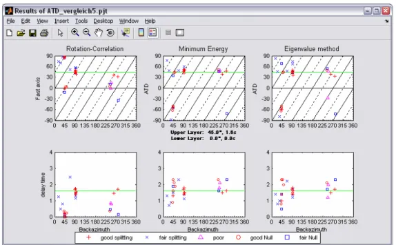
SplitLab est fournis avec un exemple de données de la station ATD (Arta Cave, Djibouti) du réseau GEOSCOPE (Figure C). Le choix de cette station a été guidé par la qualité des données que l'on y trouve, la clarté de la direction anisotrope rapide, l'amplitude du déphasage temporel, et le consensus existant sur les paramètres de déphasage obtenu à partir de diverses études d'anisotropie publiées à cette station [Vinnik et al., 1989 ; Barruol et Hoffmann, 1999].

Figure B: Les résultats de la station ATD avec SplitLab. La comparaison des trois techniques différentes est possible très facilement

0

0 .

.

2

2 .

.

C

r

i

t

è

r

e

d

e

“

N

u

l

”

Lors des mesures de déphasage d'ondes de cisaillement, de nombreux événements ne présentent pas de déphasage, l'énergie des ondes sismiques étant concentrée sur la composante radiale. Ce type de mesure est généralement caractérisé de "null" dans la littérature mais représente en fait une information importante. Je présenterai un nouveau critère pour distinguer sûrement des événements « Nulls » (chapitre 4.4). Ce critère est basé sur la comparaison des deux techniques indépendantes de mesure de déphasages des ondes S. Un test avec des sismogrammes synthétiques montre que un différence caractéristique entre la technique « Rotation-Correlation » [RC, Bowman et Ando, 1997] and « energie minimal sur la composant transverse » [SC, Silver et Chan, 1991].

Les deux techniques donnent des valeurs correctes si les backazimuths sont suffisamment loin des axes rapides (ou lents). Près de ces directions "Nulls", il y a des déviations caractéristiques, particulièrement pour la technique « Rotation-Correlation ». Les valeurs du δtRC diminuent systématiquement, alors que ΦRC montre des déviations d’environ 45º

(15)

pour avoir une corrélation maximale entre les deux composants horizontaux Q (radial) et T (transversal). Je montrerai que cette technique faillit en cas des Nulls car le signal sur T est minimal. La technique trouve la meilleure corrélation à 45°, ou le maximum d'énergie de la composante Q est “copié” vers la composante T.

Les différences caractéristiques des résultats issus de ces deux techniques ne permettent pas seulement de différencier les Nulls des non-Nulls mais également d'assigner une qualité objective à une mesure individuelle. Cette quantification pourrait par la suite permettre de comparer différentes études. Ces critères sont appliqués à la station LVZ en Scandinavie où les résultats sont définis avec une plus grande certitude qu'auparavant, malgré une couverture backazimuthale très faible.

−90 −45 0 45 90 −90 −45 0 45 90 fast axis

Rotation correlation method

−90 −45 0 45 90 −90 −45 0 45 90

Minimum energy method

−900 −45 0 45 90 1 2 3 4 Backazimuth delay time −900 −45 0 45 90 1 2 3 4 Backazimuth

Figure A: Test synthétique à SNRR = 15 pour la technique de Rotation-Corrélation (RC, gauche) et la technique minimum d'énergie (SC, droite). Les panneaux supérieurs montrent les haches rapides résultantes à différents backazimuths, expositions inférieures de panneaux que résulter

(16)

0

0 .

.

3

3 .

.

B

a

s

e

d

e

s

d

o

n

é

e

s

d

e

«

s

h

e

a

r

w

a

v

e

s

p

l

i

t

i

n

g

»

Le nombre de plus en plus important des études de déphasage des ondes S a été une motivation pour centraliser les données (chapitre 4.6) de déphasage des ondes de cisaillement publiées dans la littérature. Basée sur une collection statique commencée par Derek Schutt et Matt Fouch, cette base de données interactive permet l'accès par l'intermédiaire d'un web browser. Les chercheurs peuvent ainsi saisir leurs propres donnés et augmenter la base de données. L'interaction avec GoogleEarth, un outil employé couramment des SIG 3D, fournit une visualisation rapide avec différents ensembles de données.

Montagner et al. [2000] ont présente une méthode a calculer les paramètres théorétique a partir des résultats de la tomographie des ondes de surface. En utilisant le model global de Debayle et al [2005] une comparaison des paramètres théorétique avec la base des donnes montre une corrélation général de les deux methodes.

0

0 .

.

4

4 .

.

L

'

a

n

i

s

o

t

r

o

p

i

e

d

u

C

r

a

t

o

n

E

s

t

E

u

r

o

p

é

e

n

Le chapitre 5 est focalisé sur l'anisotropie dans des régions cratoniques. D'abord, une vue d'ensemble générale sur la structure et l'évolution des cratons est présentée (chapitre 5.1), suivi d'un rappel des études de déphasage des ondes S sur des cratons (chapitre 5.2). Le chapitre 5.3 reprend l'évolution et les propriétés géophysiques du craton Est Européen et je présente dans la section 5.4 les mesures de déphasage effectuées dans cette thèse avec les techniques et outils précédemment présentés.

Le craton de l'Europe de l'Est (CEE) se compose de trois segments de croûte principaux: Fennoscandia, Sarmatia et Volgo-Uralia. Aujourd'hui, le CEE est largement recouvert par des sédiments du Phanerozoic. Seuls les boucliers de Fennoscandia et les parties sud du Bouclier Ukrainien et du Massif de Voronezh offrent à l'affleurement des roches protérozoïques et plus anciennes [Gorbatschev et Bogdanova 1993 ; Bogdanova, 1996]. Entre 2.1Ga et 2.0, le domaine océanique, qui séparait Sarmatia de Volgo-Uralia, s'est fermé. Simultanément, la subduction commencée sur le bord (actuel) nordique de Sarmatia se finit à environ 1.8Ga à la collision avec Fennoscandia. La réunion des deux blocs a eu lieu à environ 1.75Ga et est accompagnée d'« underplating ».

Un total de 16 stations sismologiques distribuées sur les multiples unités tectoniques du CEE sont analysées dans cette étude. Les axes rapides montrent de fortes variations pour chaque unité tectonique, suggérant une anisotropie « gelée » dans la lithosphère.

(17)

Figure D: Mesures de déphasages des ondes S en Europe. Les marqueurs gris représentent des mesures de la base de données SKS. Les marqueurs bleus et verts sont issus de cette étude, et représentent (lorsqu'elles semblent présentes), les couches anisotropes supérieure et inférieure respectivement. PLB="terrane" Polonais-Lituanien-Bélarus ; TTZ=Tesseyre-Tornquist zone

Une telle interprétation est soutenue par une corrélation variable des axes rapides avec la direction de mouvement de la plaque, qui ne montre pas de parallélisme systématique et qui ne semble pas refléter les processus asthénosphériques actuels à grande échelle. En Fennoscandia, les axes rapides montrent des directions NS dans le bloc Karélien au nord, et NE-SW dans Svecofennia près de St. Petersburg. C'est en accord avec les résultats obtenus en Finlande [Plomerova et al., 2005]. La corrélation faible avec la direction de mouvement de la plaque Eurasie suggère des origines lithosphériques plutôt qu'asthénosphériques.

(18)

reflèteraient donc plutôt des directions anciennes de mouvement de la plaque pendant la subduction de Volgo-Uralia dans cette région.

Dans Samartia, les stations ne rapportent aucune orientation rapide logique d'axes rapides. Dans le NE, les deux stations OBN et MHV semblent indiquer une superposition complexe de cas d'hétérogénéité et de deux-couche d'anisotropie, provenant du massif de Voronezh et de la dorsale de Pachelma. À l'ouest, la station KIEV montre beaucoup de "Nulls" avec une gamme étendue de backazimuths. Ceci pourrait indiquer la présence de deux couches anisotropes mutuellement perpendiculaires ou bien l'absence d'anisotropie sous la station. Pour KIEV, il semble probable que la superposition de plusieurs événements tectoniques a finalement effacé les orientations préférentielles existantes des minéraux. Ceci expliquera le grand nombre des Nulls de un grande gamme des backazimuths.

Les orientations des axes rapides observées aux stations le long de la zone de suture de Tesseyre-Tornquist (TTZ) s'alignent avec les axes raides en Europe centrale. Ceci peut indiquer que les mêmes processus sont responsables de l'anisotropie de chaque côté de la zone de suture. Un processus possible pourrait être un flux de manteau, guidé et dévié par la lithosphère plus épaisse du CEE. Les études tomographiques indiquent en effet que l'augmentation de l'épaisseur lithosphérique coïncide avec le TTZ.

(19)

(20)

1.

1. TT

T

TT

T

h

e

ssss

iiii

ssss

M

o

tttt

iiii

vvvv

a

tttt

iiii

o

n

Seismic waves are arguably the most powerful geophysical tools to investigate the Earth’s deep interior. Sensitive to compositional changes and sharp contrasts, a seismic wave arriving at a recording station contains the whole suite of information acquired along its travel path. Source mechanisms can be studied at stations far away from the earthquakes, which gives information about the source region. A seismic wave is furthermore sensible to the elastic varying properties along its travel path. Consequently, the inversion of a seismic wave (body wave, surface wave, free oscillations) permits interpretations of the Earth’s inner structure.

One of the many material properties affecting seismic waves is anisotropy. Identifying the orientation of seismic anisotropy and eventually interpreting its origins by comparison with surface tectonic features is aimed at understanding tectonic processes acting within the Earth.

Seismic anisotropy is the dependence of wave speed on direction. Such anisotropy can be caused by structural variability such as thin layers of alternating elastic properties [Backus, 1962] or fluid filled cracks [Crampin, 1984; Kendall et al., 2006]. A second origin of anisotropy is the preferred orientation of anisotropic minerals by strain [e.g., Nicolas & Christensen, 1987]. It is widely accepted, that the preferred orientations of olivine minerals play a major role in the anisotropy of the Earth’s mantle.

Perhaps the best indicator of seismic anisotropy are split waves. A seismic shear-wave passing through an anisotropic medium is split in two shear-waves, polarized parallel to the anisotropic directions and travelling at different velocities. At the surface, they thus arrive separated by a certain delay time. In optics this effect is know as bifringence. Seismic shear-wave splitting has been studied for decades. Initially limited to direct S waves from local events [Ando & Ishikawa, 1982], the technique is now widly adopted for core-transiting phases such as SKS, SKKS, PKS [e.g., Vinnik et al., 1984, Silver and Chan, 1991]. Over the past two decades the method of shear-wave splitting has been

(21)

widely applied in several geologic settings: Subduction zones [e.g., Levin et al., 2004; Margheriti et al., 2003; Nakajima & Hasegawa, 2004], rifts [Kendall, 1994; Gao et al., 1997; Walker et al., 2004; Kendall, 2005], hotspots [Barruol & Granet, 2002; Walker et al., 2001; 2005], oceanic islands [Behn et al., 1999; Fontaine et al., 2007] and orogens [e.g., Barruol et al., 1998; Flesch et al., 2005].

Using teleseismic phases allows measurements at large distances from seismically active regions such as cratons. Cratons form the thick, stable interiors of the continents and their roots may act as obstacles to mantle flow [Fouch et al., 2000]. Analyzing anisotropy in such environments may help to distinguish this present day deformation, associated with plate motion, from fossil deformation. Several studies analyzed anisotropy beneath the various cratons [Fouch et al., 2000; Heintz & Kennett, 2005; Fouch & Rondenay, 2006; Assumpção et al. 2006].

Ever larger temporary arrays (e.g. USarray) and long running permanent stations make the available datasets grow fast. Shear wave splitting has thus become over last decade a quasi standard technique to perform at a seismic broad band station. This evokes the need for a splitting environment which is efficient and easy-to-use while still flexible enough to be applied to several problems.

The aim of this study was to develop such a shear-wave splitting environment, SplitLab, which is then applied to stations on the East European Craton. Matlab was chosen as the underlying code since it provides a great flexibility in operating systems and its scripting language can be readily adapted to specific problems. Furthermore, the possibilities to incorporate Graphical User Interfaces (GUIs) make SplitLab a modern, user-friendly and effective environment. SplitLab is intended to undertake the repetitive processing steps while enabling the user to focus on quality control and eventually the interpretation of the results.

The powerful possibilities of SplitLab are applied to stations on the East European Craton (EEC) for several reasons: first, from a geological point of view the Platform as a whole has yet not been investigated. Some of these stations have already been processed independently or within another framework [Silver & Chan, 1991; Makeyeva et al. 1992; Helffrich et al., 1994; Dricker et al, 1999]. A regional analysis of upper mantle anisotropy

(22)

to every code. And finally, a broad range of recording times (e.g., 15 years for KIEV and 18 month for NE53) and varying data quality provide a good synopsis of the generally accounted situations during shear wave splitting.

1

1 .

.

1

1 .

.

T

h

e

s

i

s

o

u

t

l

i

n

e

This thesis will first point out the fundamental physics of seismic wave propagation, with a particular focus on anisotropic media [Chapter 2]. In Chapter 3, the different origins of anisotropy will be discussed. In general, anisotropy can be divided into to classes: (small-scale) crystalline anisotropy and (large-(small-scale) structural anisotropy. The possible depths where anisotropy can occur are discussed as well as the effects of different tectonic settings.

The technical aspects of shear-wave splitting are presented in Chapter 4. The simultaneous application of the different splitting techniques is performed using the newly developed splitting environment SplitLab (Chapter 4.3). This graphical environment encompasses the whole splitting process from earthquake selection to seismogram request to data processing and finally results overview. Several graphical user interfaces (GUIs) make the usage intuitive.

I will present a novel criterion to reliably distinguish splitting events from so-called Nulls (Chapter 4.4). This criterion is based on the comparison of two genuinely different splitting techniques. Characteristic differences in their results allow not only to differentiate Nulls from non-Nulls but also to assign an objective quality to an individual measurement. This objectiveness might eventually enhance comparability between different studies.

A short outlook of how to possibly automate the whole splitting procedure of a seismic station is presented in Chapter 4.5.

The growing number of shear-wave splitting studies motivated to create a central collection of splitting data (Chapter 4.6). Based on a static text-file collection started by Derek Schutt and Matt Fouch, the Interactive Shear-Wave Splitting Database allows access via a web-browser. Most important, researchers can enter their own data so that at each time the newest studies are available. Interaction with GoogleEarth, a widely used 3D GIS tool, allows for fast visual comparison with different datasets.

Finally, Chapter 5 discusses anisotropy in cratonic regions. First, a general overview on the structure and evolution of cratons is presented (Chapter 5.1), followed by a short review of shear-wave splitting studies on cratons (Chapter 5.2). Chapter 5.3 resumes the evolution and the geophysical properties of the East European Craton. This is followed in Chapter 5.4 with the results of shear-wave splitting measurements performed in this thesis.

(23)

analysis of coherence within and variability between these units. It is proposed to compare the (lithospheric) anisotropy with aeromagnetic data. Aeromagnetic data allow the detection of crustal structural trends and compositional changes in regions, whose geologies are only poorly constrained or covered by sediments.

(24)

2.

2. L

L

iiii

n

e

a

rrrr

e

llll

a

ssss

tttt

iiii

cccc

iiii

tttt

yyyy

a

n

d

w

a

vvvv

e

p

rrrr

o

p

a

g

a

tttt

iiii

o

n

Whenever a force is applied to a continuum, every point of this continuum is influenced by the force. Internal forces are commonly referred to as body forces while external forces are denoted contact forces. The most common example for a body force is acceleration due to gravity. Body forces are proportional to volume and density of the medium they are applied to. Contact forces depend on the area they are acting on.

In general, any external force applied to a continuum will deform the medium in size and shape. Internal forces try to resist this deformation. As a consequence the medium will return to its initial shape and volume once the external forces are removed. If this recovery of the original shape is perfect the medium is called elastic. The constitutive law relating

the applied force with the resulting deformation is Hooke’s Law, named after the 17th

century physicist Robert Hooke (1635–1703). It is defined in terms of stress and strain. Many books have been written about this topic. This chapter is mainly based on Ranalli [1995] and Turcotte & Schubert [2002] for the stress/strain parts, and Stein & Wysession [2003], Lay & Wallace [1995] and Shearer [1999] for the seismic anisotropy. A detailed theory of wave propagation in anisotropic media is given for example by Tsvankin [2001]. To quantify the state of stress at a point P resulting from a forceF

r

, P is imagined as an infinitesimal small cube, each side having an infinitesimal small surface δS. The traction

T r

acting can be decomposed into its stress components normal (σh and tangential (σh) to

this surface. The latter can be further decomposed into components parallel to the coordinate axes (Figure 1).

(25)

Figure 1: Components of stress acting on a surface. Any traction can be divided into its components normal and tangential to the surface. The latter can be further decomposed into two components parallel to the coordinate axes.

A stress σij is defined as acting on the i-plane and being oriented in j-direction.

Consequently, the components with repeating indices are normal stresses, while different indices indicate shear stresses (Figure 2). If the medium is in static equilibrium the sum of all stress components act in the 1, 2, and 3 directions as well as the total moment is zero. This symmetry is expressed as:

σij = σji

Thus, six independent parameters of the stress tensor σij completely describe the state of stress at any point P of this continuum:

          =           = 33 32 13 23 22 12 13 12 11 33 23 31 23 22 21 13 12 11

σ

ij , with i, j = 1, 2, 3

(26)

As mentioned above, an elastic body subjected to stress deforms. By definition, this deformation is called the strain ε. It is the (dimensionless) relative change in dimension of a body. In the three-dimensional case with deformations sufficiently small this is described by the infinitesimal strain tensor

          =           = 33 32 13 23 22 12 13 12 11 33 23 31 23 22 21 13 12 11

ε

ij , with i, j = 1, 2, 3

where the same symmetry considerations as for the stress tensor reduce the number of independent components to six:

εij = εji

2

2 .

.

1

1 .

.

H

o

k

e

’

s

L

a

w

Stress and strain are related to each other by Hooke’s Law, which assumes the strains to be sufficiently small and that stress and strain depend linearly on each other. Such a

medium is called linear elastic. In its general form it can be written as

kl ijkl ij C ε

σ = , with i, j, k, l = 1, 2, 3

The fourth-order tensor Cijkl is called the stiffness tensor, which consists of 81 entries and

describes the elastic properties of a medium. This tensor actually links the applied stress to the resulting deformation of the medium. In general Hooke’s Law can lead to complicated relations, but symmetry considerations remarkably simplify the equations by reducing the number of independent parameters from 81 to 36:

Cijkl = Cjikl = Cijlk = Cjilk

Moreover, general thermodynamics [e.g., Nye, 1972] requires the existence of a unique strain energy potential, and therefore:

(27)

Cijkl =Cklij

which reduces the number of independent entries in the stiffness tensor to 21. These 21 parameters are necessary to fully describe the stress-strain relationship of an elastic body in its most general form. These parameters may vary with direction, in which case the medium is called anisotropic. In contrast, the properties of an isotropic medium are the same in every direction. There are seven unique symmetry systems, each representing a specific number of elastic parameters. The most complex and least symmetry is triclinic which needs the whole 21 elastic parameters to be fully described. In order of increasing symmetry the other six systems are (number of elastic parameters in brackets): monoclinic (13), orthorhombic (9), tetragonal (7, 6), trigonal (7, 6), hexagonal (5), cubic (3) and isotropic (2).

2

2 .

.

2

2 .

.

I

s

o

t

r

o

p

i

c

m

e

d

i

a

In the case of isotropy, Cijkl is invariant with respect to rotation, the number of independent

parameters reduce to two:

Cijkl = λδijδkl + µ(δikδjl + δilδjk)

where λ andµ are called the Lamé parameters and δil is the Kronecker delta. µ also

denotes the shear modulus, and describes the resistance to shearing of the medium according to

σij = 2µεij , with i ≠ j

The bulk modulus K is defined as the ratio of applied isostatic stress to the fractional volumetric change:

(28)

σij = Eεii .

Finally, the (dimensionless) Poisson’s ratio υ is also defined for uniaxial stress and relates the lateral strain to the axial strain:

ii jj

ε

υ

=−

Note that here the Einstein sum convention is not applied. Note also that υ varies only

between 0 and 0.5 with the upper limit representing a fluid (µ= 0).

In the case of an isotropic, linear elastic material, the bulk modulus, the shear modulus and

the density ρ define the compressive and shear velocities VP and VS, respectively:

ρ

µ

ρ

µ

= + = S P V K V 3 4

In the following considerations it is convenient to use Voigt’s representation of the

stiffness tensor Cijkl, which transfers the 3x3x3x3 tensor to a 6x6 matrix

                    =                     = 66 65 64 63 62 61 56 55 54 53 52 51 46 45 44 43 42 41 36 35 34 33 32 31 26 25 24 23 22 21 16 15 14 13 12 11 1212 1213 1223 1233 1222 1211 1312 1313 1323 1333 1322 1311 2312 2313 2323 2333 2322 2311 3312 3313 3323 3333 3322 3311 2212 2213 2223 2233 2222 2211 1112 1113 1123 1133 1122 1111 c c c c c c c c c c c c c c c c c c c c c c c c c c c c c c c c c c c c C C C C C C C C C C C C C C C C C C C C C C C C C C C C C C C C C C C C c_mn

For isotropic material, the stiffness matrix can be represented by only two parameters, the

(29)

                    + + + =

µ

λ

µ

λ

µ

λ

0 0 0 0 0 0 0 0 0 0 0 0 0 0 0 0 0 0 2 0 0 0 2 0 0 0 2 mn c

2

2 .

.

3

3 .

.

A

n

i

s

o

t

r

o

p

i

c

m

e

d

i

a

The more general anisotropic formulation describes the elastic properties of a material, if the variation of parameters with direction is allowed. Anisotropy may be due to crystal structure (Chapter 3.1) or other microscopic and macroscopic effects, e.g. layering; Chapter 3.2. Generally, either orthorhombic or hexagonal symmetry is assumed when analyzing the earth.

Hexagonal anisotropic media are characterized by a single plane of isotropy and one single axis of rotational symmetry. It can be caused either by intrinsic anisotropy of the dominant mineral (e.g. mica, clay, serpentine) or by periodic layering of materials with different elastic properties. The layers have to be thin in comparison to the seismic wavelength (Figure 3a). Hexagonal anisotropy is fully characterized by five independent

elastic parameters. If we assume that the axis of symmetry is x3 the stiffness matrix has the

form                     − − = 66 55 55 33 13 13 13 11 66 11 13 66 11 11 0 0 0 0 0 0 0 0 0 0 0 0 0 0 0 0 0 0 0 0 0 2 0 0 0 2 c c c c c c c c c c c c c c cmntrans

(30)

Figure 3: Possible origins of anisotropy (after Shearer [1999]): a) thin layered material results in hexagonal symmetry anisotropy. b) Minerals like olivine have an intrinsic anisotropy.

Orthorhombic media are characterized by three mutually orthogonal axes of symmetry. One of the most abundant mineral in the Earth’s mantle, olivine, belongs to this class (Figure 3b). If the coordinate axes coincide with the symmetry axes the stiffness matrix of the orthorhombic system has nine independent entries and has the form

                    = 66 55 44 33 23 13 23 22 12 13 12 11 0 0 0 0 0 0 0 0 0 0 0 0 0 0 0 0 0 0 0 0 0 0 0 0 c c c c c c c c c c c c cortho_mn

Olivine is an anisotropic mineral and a main composite of the (upper) mantle. It has a

density of 3.311 kg/m3. The elastic tensor (in GPa) of this orthorhombic mineral is

[Kumazawa & Anderson, 1969]:

(31)

                    = 0 . 79 0 0 0 0 0 0 7 . 78 0 0 0 0 0 0 6 . 64 0 0 0 0 0 0 1 . 235 6 . 75 6 . 71 0 0 0 6 . 75 6 . 197 4 . 66 0 0 0 6 . 71 4 . 66 7 . 323 ij c

Figure 4: velocities of olivine in the lower hemisphere.

2

2 .

.

4

4 .

.

P

l

a

n

e

w

a

v

e

p

r

o

p

a

g

a

t

i

o

n

Plane waves play an essential part in understanding wave propagation. Here, the

displacement only varies in the direction of wave propagation. The displacement urat

(32)

where sr=nˆ/V is the slowness vector, whose magnitude is reciprocal to the velocity V, nˆ is an unit vector, t is time and f

r

is an arbitrary function representing the wave form. A harmonic plain wave with angular frequency ω is represented by

) / ˆ ( ) ( ) , (x t A e i nx V t u = − − r r r r _ω

ω

The (elastic) wave propagation is governed by Hooke’s Law. Written as a differential equation, the plane wave is described as

0 2 2 2 = ∂ ∂ ∂ − ∂ ∂ l j k ijkl i x x u C t u

ρ

where ρ is the density of the medium, ui is the displacement vector, and xi are the

Cartesian coordinates. Summation over repeated indices is implied. Note that anisotropy enters the equation via the stiffness tensor Cijkl. Inserting this Ansatz in this differential

equation gives the Christoffel equation, named after the German mathematician Elwin Bruno Christoffel (1829–1900)

0 )

(M_ik −

ρ

V2

δ

_ik E_k =

Mij is the Christoffel matrix, which is a function of the material properties and direction of

wave propagation: i j ijkl ij C n n M =

The Christoffel equations describes a standard eigenvalue (ρV2) – eigenvector (Ei)

problem, where the eigenvalues are determined by

0 ) det(M_ij −ρV2δ_ij =

(33)

The solution of this cubic equation yields three possible values of the squared velocity V, namely one P-wave and two S-wave velocities (e.g., SH and SV). As shown before

(Chapter 2.2), the two S wave velocities are identical in isotropic media and we get

ρ µ β ρ µ λ α = = + = iso = S iso P V V 2 ;

For any specific direction ni in an anisotropic medium, these are represented by the three

eigenvalues. The three eigenvectors specify the polarization of the wave, namely the quasi-P, the fast S-wave, and slow S-wave. Backus [1965] showed that for weak anisotropy the velocities in dependence on azimuth θ can be approximated to first order as

θ

2 sin 2 cos 4 sin 4 cos 4 sin 4 cos 2 sin 2 cos 2 2 || 2 s c S s c S c c s c P G G F V E E D V C C B B A V + + = + + = + + + + = ⊥

where VP is the P-wave velocity, VS|| and V_S_⊥are the S-wave velocity parallel and

perpendicular to symmetry plane, respectively. The coefficients depend on the elastic constants: 1212 1122 4 1 2222 1111 8 1 1222 2111 2 1 1212 1122 4 1 2222 1111 8 1 1222 2111 2222 1111 2 1 1212 1122 4 1 2222 1111 8 3 ) 2 ( ) ( ) ( ) 2 ( ) ( ), ( ), ( ) 2 ( ) ( C C c C D C C C C C c C C C C B C C B C C c C A s c s c − − + = − = + − + = + = − = + + + =

(34)

2

2 .

.

5

5 .

.

S

e

i

s

m

o

l

o

g

i

c

a

l

d

e

t

e

c

t

i

o

n

o

f

a

n

i

s

o

t

r

o

p

y

2

2 .

.

5

5 .

.

1

1 .

.

P

-

w

a

v

e

s

Early measurements of Pn velocities as a function of azimuth in the oceans revealed higher velocities perpendicular to the mid ocean ridges [e.g., Morris et al., 1969]. These measurements showed a strong 2θ dependency, as described before [Backus, 1965]. More general, the arrival of P-waves depends on azimuth and incident angle (Figure 4). The depth integral along all ray paths yields the delay time variations (Figure 5). Therefore, the study of teleseismic P delays reveals the anisotropic structure beneath a station. Bokelmann [2002a, 2002b] uses this technique to determine the 3D orientation of anisotropy beneath North America. Babuska & Plomerova [1996] propose a joint inversion of P-wave and Shear wave splitting (see below).

Figure 5: a) Ray geometry through an anisotropic block of dipping anisotropy. The fast axis is dipping 30° to the SW, the intermediate axis is dipping 60° to the NE, and the slow axis is horizontal. b) The lower hemisphere shows predicted fast/slow delays (crosses and circles respectively; given in sec) for a propagation through a 150 km anisotropic layer defined in a). [after Bokelmann, 2002b]

The analysis of polarizations of quasi-P waves has also proposed by Bokelmann [1995] and Schulte-Pelkum et al. [2001; 2003]. The horizontal polarization of the initial P particle motion can deviate by >10° from the predicted azimuth along a great circle from station to source. They showed that stations within regional distances of each other show consistent azimuthal deviation patterns, while the deviations seem to be independent of source depth and near-source structure.

2

2 .

.

5

5 .

.

2

2 .

.

S

h

e

a

r

w

a

v

e

s

p

l

i

t

i

n

g

(35)

surface stations by recovering their original polarization gives information about the anisotropic medium. This is the subject of this thesis.

Montagner et al. [2000] present a derivation of this phenomenon. These equations have been described before by Vinnik et al. [1989] and Silver & Chan [1991]. Let us consider now the simplest case: a vertically propagating S-wave within an isotropic medium. The associated displacements in wave coordinate system (Radial, Transverse, and Vertical) are then        = = − = = − 0 0 )) ( exp( ) , ( 0 0 0 z T Vs z z R iso u u t i a u t z u ω

where Vs0(z) is the S-wave velocity in the isotropic medium. In a geographic coordinate

system the displacements are

       = − Ψ = − Ψ = = − − 0 )) ( exp( sin )) ( exp( cos ) , ( 0 0 0 0 0 0 z Vs z z N Vs z z E iso u t i a u t i a u t z u

ω

where Ψ is the backazimuth. Now assume, that at depth z = z0 the wave enters an

anisotropic medium with horizontal (fast and slow) symmetry axes. This reduces the problem to two dimensions, since the vertical axis is identical to all appearing systems. Let ΨA be the angle between North and the orientation of the fast S-wave polarization

(36)

2 0 V

Vs −δ and thus accumulating a delay. This is expressed in the “dephasing matrix”

      = i+ _i₋ e e H 0 0

, whose elements ei± can be rewritten as

      −       − − ± ₌ 2 0 0 0 0 2 ) ( S V V z z i Vs z z i i e e e δ ω ω m .

The second exponential term can be developed into a Taylor Series if

ω(z-z0)(δV/2V2s0) << 1. This is achieved for signal periods T=2π/ω larger than

approximately 3s, assuming an anisotropy of 5% (δV/Vs0=0.05), an average S-wave

velocity of Vs0 = 4km/s and a thickness of the anisotropic layer of 100km. Therefore, a

first order approximation is valid for small anisotropies and body waves of long periods (T>10s). SKS waves are ideal for this analysis, since their dominant period is usually approximately 8 seconds, and their arrival is well separated from other phases.

A rotation of the displacement vector from the anisotropic system (f-s) into the wave coordinate system (R-T) yields

(

)

2 0 0 0 0 2 0 0 2 0 0 0 0 2 ) ( / 0 2 ) ( / 2 ) ( 0 0 / 2 2 1 / 2 / 2 sin 2 sin sin 2 cos cos sin sin cos ) , ( Vs V z z A Vs z z t i T Vs V z z A Vs V z z Vs z z t i R t i i i A i A i A T R aniso e a u i e a u e a e e e e u u t z u δ ω ω δ ω δ ω ω ω

ψ

−       ₋ − − −       ₋ − − + − + =       ₊ =         + + =       =

where

ψ

_A/ =

ψ

_A−

ψ

is the angle between fast axes and North. Reordering and taking advantage of the fact that if ω(z-z0)(δV/2V2s0) << 1 the components of displacement after

the anisotropic layer in wave coordinate system are

0 / 2 1 0 / 2 sin ) ( ) 2 cos 1 ( ) ( R A t i T R A t i R u t e t u u t i e t u &

ψ

δ

ψ

ωδ

ω ω = + =

(37)

where δt = (z-z0)(δV/2V2s0) is the accumulated delay time, and u&R0 =∂uR0 /∂t=i

ω

uR0is the

time derivative of the waveform before the anisotropic layer (u_T0 =0).

2

2 .

.

5

5 .

.

3

3 .

.

S

u

r

f

a

c

e

w

a

v

e

s

In isotropic, laterally homogeneous media two types of surface waves exist (Figure 6): Love waves have rectilinear particle motion in a horizontal plane perpendicular to propagation direction. Rayleigh waves show elliptical particle motion in a vertical plane along propagation direction.

Surface waves propagate parallel to the surface of the earth. The penetration depth is proportional to their wavelength. For this reason, different modes of a surface wave travel at different velocities (reflecting the velocity structure of the Earth), leading to a dispersion of the signal. This can in turn be used to study the depth structure of the Earth. However, the long wave lengths limit the lateral resolution (~400km; [Debayle et al., 2005])

Figure 6: Sketch of the particle motion of Love and Rayleigh waves (after Lay & Wallace, 1995)

Discrepancies in dispersion curves of Love and Rayleigh waves can be well explained by hexagonal anisotropy with a vertical axis of symetry. Smith & Dahlen [1973] showed that the equation of azimuthal phase-velocity variations for Love and Rayleigh waves at a given period has a form similar to (quasi-) P waves:

θ θ θ θ θ θ ≈ = + + + +